1243
A Stochastic Decoder for Neural Machine Translation
∗Philip Schulz
Amazon Research†
Wilker Aziz
University of Amsterdam
Trevor Cohn
University of Melbourne
Abstract
The process of translation is ambiguous, in that there are typically many valid trans-lations for a given sentence. This gives rise to significant variation in parallel cor-pora, however, most current models of machine translation do not account for this variation, instead treating the prob-lem as a deterministic process. To this end, we present a deep generative model of machine translation which incorporates a chain of latent variables, in order to ac-count for local lexical and syntactic varia-tion in parallel corpora. We provide an in-depth analysis of the pitfalls encountered in variational inference for training deep generative models. Experiments on sev-eral different language pairs demonstrate that the model consistently improves over strong baselines.
1 Introduction
Neural architectures have taken the field of ma-chine translation by storm and are in the pro-cess of replacing phrase-based systems. Based on the encoder-decoder framework (Sutskever et al., 2014) increasingly complex neural systems are being developed at the moment. These systems find new ways of extracting information from the source sentence and the target sentence prefix for example by using convolutions (Gehring et al., 2017) or stacked self-attention layers (Vaswani et al.,2017). These architectural changes have led to great performance improvements over classical RNN-based neural translation systems (Bahdanau et al.,2014).
∗Code and a workflow that reproduces the experiments are available at https://github.com/philschulz/ stochastic-decoder.
†Work done prior to joining Amazon.
Surprisingly, there have been almost no efforts to change the probabilistic model wich is used to train the neural architectures. A notable exception is the work ofZhang et al.(2016) who introduce a sentence-level latent Gaussian variable.
In this work, we propose a more expressive latent variable model that extends the attention-based architecture ofBahdanau et al.(2014). Our model is motivated by the following observation: translations by professional translators vary across translators but also within a single translator (the same translator may produce different translations on different days, depending on his state of health, concentration etc.). Neural machine translation (NMT) models are incapable of capturing this variation, however. This is because their likeli-hood function incorporates the statistical assump-tion that there is one (and only one) output1for a
given source sentence, i.e.,
P(y1n|xm1 ) =
n ∏
i=1
P(yi|xm1 , y<i). (1)
Our proposal is to augment this model with la-tent sources of variation that are able to represent more of the variation present in the training data. The noise sources are modelled as Gaussian ran-dom variables.
The contributions of this work are:
• The introduction of an NMT system that is capable of capturing word-level variation in translation data.
• A thorough discussions of issues encountered when training this model. In particular, we motivate the use of KL scaling as introduced byBowman et al.(2016) theoretically.
1Notice that from a statistical perspective the output of an
• An empirical demonstration of the improve-ments achievable with the proposed model.
2 Neural Machine Translation
The NMT system upon which we base our exper-iments is based on the work of Bahdanau et al. (2014). The likelihood of the model is given in Equation (1). We briefly describe its architecture. Letxm1 = (x1, . . . , xm)be the source sentence and yn1 the target sentence. Let RNN(·) be any function computed by a recurrent neural network (we use a bi-LSTM for the encoder and an LSTM for the decoder). We call the decoder state at the
ith target positionti; 1≤i≤n. The computation
performed by the baseline system is summarised below.
[
h1, . . . , hm]=RNN(xm1 ) (2a)
˜
ti=RNN(ti−1, yi−1) (2b)
eij =v⊤a tanh (
Wa[˜ti, hj]⊤+ba )
(2c)
αij =
exp(eij) ∑m
j=1exp(eij)
(2d)
ci=
m ∑
j=1
αijhj (2e)
ti=Wt[˜ti, ci]⊤+bt (2f )
ϕi=softmax(Woti+bo) (2g)
The parameters {Wa, Wt, Wo, ba, bt, bo, va} ⊆ θare learned during training. The model is trained using maximum likelihood estimation. This means that we employ a cross-entropy loss whose input is the probability vector returned by the softmax.
3 Stochastic Decoder
This section introduces our stochastic decoder model for capturing word-level variation in trans-lation data.
3.1 Motivation
Imagine an idealised translator whose translations are always perfectly accurate and fluent. If an MT system was provided with training data from such a translator, it would still encounter variation in that data. After all, there are several perfectly accurate and fluent translations for each source sentence. These can be highly different in both their lexical as well as their syntactic realisations.
In practice, of course, human translators’ per-formance varies according to their level of educa-tion, their experience on the job, their familiarity with the textual domain and myriads of other fac-tors. Even within a single translator variation may occur due to level of stress, tiredness or status of health. That translation corpora contain variation is acknowledged by the machine translation com-munity in the design of their evaluation metrics which are geared towards comparing one machine-generated translation against several human trans-lations (see e.g.Papineni et al.,2002).
Prior to our work, the only attempt at mod-elling the latent variation underlying these differ-ent translations was made by Zhang et al.(2016) who introduced a sentence level Gaussian variable. Intuitively, however, there is more to latent varia-tion than a unimodal density can capture, for ex-ample, there may be several highly likely clusters of plausible variations. A cluster may e.g. consist of identical syntactic structures that differ in word choice, another may consist of different syntactic constructs such as active or passive constructions. Multimodal modelling of these variations is thus called for—and our results confirm this intuition.
An example of variation comes from free word order and agreement phenomena in morphologi-cally rich languages. An English sentence with rigid word order may be translated into several or-derings in German. However, all oror-derings need to respect the agreement relationship between the main verb and the subject (indicated by underlin-ing) as well as the dative case of the direct object (dashes) and the accusative of the indirect object (dots). The agreement requirements are fixed and independent of word order.
1. I can’t imagine you naked.
(a) Ich kann mir . . . .dich nicht nackt vorstellen. (b) Ich kann . . . . .dich mir nicht nackt vorstellen. (c) . . . . .Dich kann ich mir nicht nackt vorstellen. Stochastically encoding the word order variation allows the model to learn the same agreement phe-nomenon from different translation variants as it does not need to encode the word order and agree-ment relationships jointly in the decoder state.
Further examples of VP and NP variation from an actual translation corpus are shown in Figure1.
预计听证会将进⾏两天。 VOM19981105_0700_0262
The hearing is expected to last two days. The hearing will last two days.
The hearings are expected to last two days.
It is expected that the hearing will go on for two days.
众议院共和党的起诉⼈则希望传唤莱温斯基等多达15个⼈出庭作证。 VOM19981230_0700_0515
However, the Republican complainant in the House wanted to summon 15 people including Lewinsky to testify in court.
The prosecutor of Republican Party in House of Representative hoped to summons more than 15 persons, including Lewinsky, to court.
The House of Representatives republican prosecution hopes to summon over fifteen witnesses includ-ing Monica Lewinsky to appear in court.
Figure 1: Examples from the multiple-translation Chinese corpus (LDC2002T01), where the translations come from different translators. These demonstrate the lexical variation of the verb and variation between passive and raising structures (top), and lexical variation on the agent NP (bottom). Both examples also exhibit appreciable length variation.
3.2 Model formulation
The model contains a latent Gaussian variable for each target position. This variable depends on the previous latent states and the decoder state. Through the use of recurrent networks, the condi-tioning context does not need to be restricted and the likelihood factorises exactly.
P(y1n|xm1 ) =
∫
dz0np(z0|xm1 )×
n ∏
i=1
p(zi|z<i, y<i, xm1 )P(yi|z1i, y<i, xm1 )
(3)
As can be seen from Equation (3), the model also contains a 0th latent variable that is meant to initialise the chain of latent variables based solely on the source sentence. Contrast this with the model ofZhang et al.(2016) which usesonlythat 0th variable.
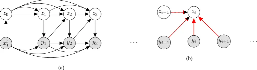
A graphical representation of the stochastic de-coder model is given in Figure2a. Its generative story is as follows
Z0|xm1 ∼ N(µ0, σ20) (4a)
Zi|z<i, y<i, xm1 ∼ N(µi, σ2i) (4b)
Yi|z0i, y<i, xm1 ∼Cat(ϕi) (4c)
where i = 1, . . . , n and both the Gaussian and the Categorical parameters are predicted by neural network architectures whose inputs vary per time step. This probabilistic formulation can be imple-mented with a multitude of different architectures. We present ours in the next section.
3.3 Neural Architecture
Since the model contains latent variables and is parametrised by a neural network, it falls into the class of deep generative models (DGMs). We use a reparametrisation of the Gaussian variables (Kingma and Welling,2014;Rezende et al.,2014; Titsias and Lázaro-Gredilla,2014) to enable back-propagation inside a stochastic computation graph (Schulman et al., 2015). In order to sample d -dimensional Gaussian variablez∈Rdwith mean µand varianceσ2, we first sample from a standard Gaussian distribution and then transform the sam-ple,
z=µ+σ⊙ϵ ϵ∼ N(0,I) . (5)
Here µ, σ ∈ Rd and ⊙ denotes element-wise multiplication (also known as Hadamard product). See the supplement for details on the Gaussian reparametrisation.
We use neural networks with one hidden layer with a tanh activation to compute the mean and standard deviation of each Gaussian distribution. A softplus transformation is applied to the output of the standard deviation’s network to ensure pos-itivity. Let us denote the functions that these net-works compute byf.
For the initial latent state z0 we compute the mean and standard deviation as
.
. xl
1
. z0
. y1
.
z1
. y2
.
z2
. y3
.
z3
(a)
. .
zi−..1 zi
yi−1 .
yi
.
yi+1
.
. . .
.
. . .
[image:4.595.91.517.70.187.2](b)
Figure 2: Graphical representation of2athe generative model and2bthe inference model. Black lines indicate generative parameters (θ) and red lines variational parameters (λ). Dashed red-black lines indi-cate that the inference model uses feature representations computed by the generative model as inputs. Through the recurrent net, the generative model (2a) also conditions its outputs on all previous latent assignments. We omit these arrows to avoid clutter. The inference model (2b) is only used at training time. Dots indicate further conditioning context.
The parameters of all other latent distributions are computed by functions fµ and fσ whose inputs
vary per target position.
µi=fµ(ti−1, zi−1) σi =fσ(ti−1, zi−1) (7)
Using these values, each latent variable is sam-pled according to Equation (5). The samsam-pled latent variables are then used to modify the update of the decoder hidden state (Equation (2b)) as follows:
˜
ti =RNN(ti−1, yi−1, zi) (8)
The remaining computations stay unchanged. Notice that the latent values are used directly in up-dating the decoder state. This makes the decoder state a function of a random variable and thus the decoder state is itself random. Applying this ar-gument recursively shows that also the attention mechanism is random, making the decoder entirely stochastic.
4 Inference and Training
We use variational inference (see e.g.Blei et al., 2017) to train the model. In variational inference, we employ a variational distributionq(z)that ap-proximates the true posteriorp(z|x)over the latent variables. The distributionq(z)has its own set of parametersλthat is disjoint from the set of model parametersθ. It is used to maximise the evidence lower bound (ELBO) which is a lower bound on the marginal likelihoodp(x). The ELBO is max-imised with respect to both the model parameters
θand the variational parametersλ.
Most NLP models that use DGMs only use one latent variable (e.g.Bowman et al.,2016). Models
that use several variables usually employ a mean field approximation under which all latent vari-ables are independent. This turns the ELBO into a sum of expectations (e.g.Zhou and Neubig,2017). For our stochastic decoder we design a more flexi-ble approximation posterior family which respects the dependencies between the latent variables,
q(zn0) =q(z0) n ∏
i=1
q(zi|z<i). (9)
Our stochastic decoder can be viewed as a stack of conditional DGMs (Sohn et al.,2015) in which the latent variables depend on one another. The ELBO thus consists of nested positional ELBOs,
ELBO0+Eq(z0)[ELBO1
+Eq(z1)[ELBO2+. . .]],
(10)
where for a given target positionithe ELBO is
ELBOi =Eq(zi)[logp(yi|x
m
1 , y<i, z<i, zi)]
−KL(q(zi)||p(zi|xm1 , y<i, z<i)) .
(11) The first term is often calledreconstructionor like-lihoodterm whereas the second term is called the
KLterm. Since the KL term is a function of two Gaussian distributions, and the Gaussian is an ex-ponential family, we can compute it analytically (Michalowicz et al., 2014), without the need for sampling. This is very similar to the hierarchical latent variable model ofRezende et al.(2014).
generative model, we call this neural net the in-ference model. At training time both the source and target sentence are observed. We exploit this by endowing our inference model with a “look-ahead” mechanism. Concretely, samples from the inference network condition on the information available to the generation network (Section 3.3) and also on the target words that are yet to be pro-cessed by the generative decoder. This allows the latent distribution to not only encode information about the currently modelled word but also about the target words that follow it. The conditioning of the inference network is illustrated graphically in Figure2b.
The inference network produces additional rep-resentations of the target sentence. One represen-tation encodes the target sentence bidirectionally (12a), in analogy to the source sentence encoding. The second representation is built by encoding the target sentence in reverse (12b). This reverse en-coding can be used to provide information about future context to the decoder. We use the sym-bolsbandrfor the bidirectional and reverse target encodings, respectively. In our experiments, we again use LSTMs to compute these encodings.
[
b1, . . . , bn ]
=RNN(y1n) (12a)
[
r1, . . . , rn]=RNN(y1n) (12b)
In analogy to the generative model (Section3.3), the inference network uses single hidden layer net-works to compute the mean and standard devia-tions of the latent variable distribudevia-tions. We denote these functionsgand again employ different func-tions for the initial latent state and all other latent states.
µ0=gµ0(hm, bn) (13a)
σ0=gσ0(hm, bn) (13b) µi=gµ(ti−1, zi−1, ri, yi) (13c) σi=gσ(ti−1, zi−1, ri, yi) (13d)
As before, we use Equation (5) to sample from the variational distribution.
During training, all samples are obtained from the inference network. Only at test time do we sample from the generator. Notice that since the inference network conditions on representations produced by the generator network, a naïve appli-cation of backpropagation would update parts of the generator network with gradients computed for
the inference network. We prevent this by block-ing gradient flow from the inference net into the generator.
4.1 Analysis of the Training Procedure
The training procedure as outlined above does not work well empirically. This is because our model uses a strong generator. By this we mean that the generation model (that is the baseline NMT model) is a very good density model in and by it-self and does not need to rely on latent informa-tion to achieve acceptable likelihood values dur-ing traindur-ing. DGMs with strong generators have a tendency to not make use of latent information (Bowman et al., 2016). This problem went ini-tially unnoticed because early DGMs (Kingma and Welling, 2014; Rezende et al., 2014) used weak generators2, i.e. models that made very strong in-dependence assumptions and were not able to cap-ture contextual information without making use of the information encoded by the latent variable.
Why DGMs would ignore the latent information can be understood by considering the KL-term of the ELBO. In order for the latent variable to be in-formative about the observed data, we need them to have high mutual informationI(Z;Y).
I(Z;Y) =Ep(z,y)
[
log p(Z, Y)
p(Z)p(Y)
]
(14)
Observe that we can rewrite the mutual informa-tion as an expected KL divergence by applying the definition of conditional probability.
I(Z;Y) =Ep(y)[KL(p(Z|Y)||p(Z))] (15)
Since we cannot compute the posterior p(z|y)
exactly, we approximate it with the variational distribution q(z|y) (the joint is approximated by
q(z|y)p(y) where the latter factor is the data dis-tribution). To the extent that the variational distri-bution recovers the true posterior, the mutual in-formation can be computed this way. In fact, if we take the learned priorp(z)to be an approxima-tion of the marginal∫ q(z|y)p(y)dyit can easily be shown that the thus computed KL term is an upper bound on mutual information (Alemi et al.,2017). The trouble is that the ELBO (Equation (11)) can be trivially maximised by setting the KL-term to 0 and maximising only the reconstruction term.
2The termweak generatorhas first been coined byAlemi
This is especially likely at the beginning of train-ing when the variational approximation does not yet encode much useful information. We can only hope to learn a useful variational distribution if a) the variational approximation is allowed to move away from the prior and b) the resulting increase in the reconstruction term is higher than the increase in the KL-term (i.e. the ELBO increases overall).
Several schemes have been proposed to en-able better learning of the variational distribution (Bowman et al.,2016;Kingma et al.,2016;Alemi et al.,2017). Here we use KL scaling and increase the scale gradually until the original objective is recovered. This has the following effect: during the initial learning stage, the KL-term barely con-tributes to the objective and thus the updates to the variational parameters are driven by the signal from the reconstruction term and hardly restricted by the prior.
Once the scale factor approaches 1 the varia-tional distribution will be highly informative to the generator (assuming sufficiently slow increase of the scale factor). The KL-term can now be min-imised by matching the prior to the variational dis-tribution. Notice that up to this point, the prior has hardly been updated. Thus moving the varia-tional approximation back to the prior would likely reduce the reconstruction term since the standard normal prior is not useful for inference purposes. This is in stark contrast toBowman et al. (2016) whose prior was a fixed standard normal distri-bution. Although they used KL scaling, the KL term could only be decreased by moving the varia-tional approximation back to the fixed prior. This problem disappears in our model where priors are learned.
Moving the prior towards the variational ap-proximation has another desirable effect. The prior can now learn to emulate the variational “look-ahead” mechanism without having access to future contexts itself (recall that the inference model has access to future target tokens). At test time we can thus hope to have learned latent variable distribu-tions that encode information not only about the output at the current position but about future out-puts as well.
5 Experiments
We report experiments on the IWSLT 2016 data set which contains transcriptions of TED talks and their respective translations. We trained models to
Data Arabic Czech French German
Train 224,125 114,389 220,399 196,883
Dev 6,746 5,326 5,937 6,996
Test 2,762 2,762 2,762 2,762
Table 1: Number of parallel sentence pairs for each language paired with English for IWSLT data.
translate from English into Arabic, Czech, French and German. The number of sentences for each language after preprocessing is shown in Table1.
The vocabulary was split into 50,000 subword units using Google’s sentence piece3 software in its standard settings. As our baseline NMT sys-tems we use Sockeye (Hieber et al.,2017)4.
Sock-eye implements several different NMT models but here we use the standard recurrent attentional model described in Section2. We report baselines with and without dropout (Srivastava et al.,2014). For dropout a retention probability of 0.5 was used. As a second baseline we use our own implemen-tation of the model ofZhang et al. (2016) which contains a single sentence-level Gaussian latent variable (SENT). Our implementation differs from theirs in three aspects. First, we feed the last hid-den state of the bidirectional encoding into encod-ing of the source and target sentence into the in-ference network (Zhang et al.(2016) use the av-erage of all states). Second, the latent variable is smaller in size than the one used by (Zhang et al., 2016).5 This was done to make their model and the stochastic decoder proposed here as similar as possible. Finally, their implementation was based on groundhog whereas ours builds on Sockeye.
Our stochastic decoder model (SDEC) is also built on top of the basic Sockeye model. It adds the components described in Sections3and4. Recall that the functions that compute the means and stan-dard deviations are implemented by neural nets with a single hidden layer with tanh activation. The width of that layer is twice the size of the la-tent variable. In our experiments we tested differ-ent latdiffer-ent variable sizes and used KL scaling (see Section4.1). The scale started from 0 and was in-creased by1/20,000after each mini-batch. Thus, at
iterationtthe scale is min(t/20,000,1).
All models use 1028 units for the LSTM
hid-3https://github.com/google/sentencepiece 4https://github.com/awslabs/sockeye
5We did, however, find that increasing the latent variable
den state (or 512 for each direction in the bidirec-tional LSTMs) and 256 for the attention mechan-sim. Training is done with Adam (Kingma and Ba, 2015). In decoding we use a beam of size 5 and output the most likely word at each position. We deterministically set all latent variables to their mean values during decoding. Monte Carlo decod-ing (Gal,2016) is difficult to apply to our setting as it would require sampling entire translations.
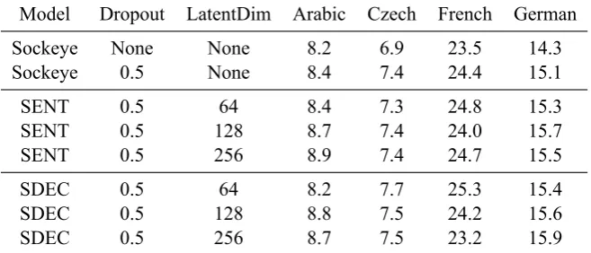
Results We show the BLEU scores for all mod-els that we tested on the IWSLT data set in Ta-ble2. The stochastic decoder dominates the Sock-eye baseline across all 4 languages, and outper-forms SENT on most languages. Except on Ger-man, there is a trend towards smaller latent vari-able sizes being more helpful. This is in line with findings byChung et al.(2015) andFraccaro et al. (2016) who also used relatively small latent vari-ables. This observation also implies that our model does not improve simply because it has more pa-rameters than the baseline.
That the margin between the SDEC and SENT models is not large was to be expected for two reasons. First, Chung et al. (2015) andFraccaro et al.(2016) have shown that stochastic RNNs lead to enormous improvements in modelling continu-ous sequences but only modest increases in perfor-mance for discrete sequences (such as natural lan-guage). Second, translation performance is mea-sured in BLEU score. We observed that SDEC of-ten reached better ELBO values than SENT indi-cating a better model fit. How to fully leverage the better modelling ability of stochastic RNNs when producing discrete outputs is a matter of future re-search.
Qualitative Analysis Finally, we would like to demonstrate that our model does indeed capture variation in translation. To this end, we randomly picked sentences from the IWSLT test set and had our model translate them several times, however, the values of the latent variables were sampled in-stead of fixed. Contrary to the BLEU-based evalu-ation, beam search was not used in this evaluation in order to avoid interaction between different la-tent variable samples. See Figure3 for examples of syntactic and lexical variation. It is important to note that we do not sample from the categori-cal output distribution. For each target position we pick the most likely word. A non-stochastic NMT system would always yield the same translation in
this scenario. Interestingly, when we applied the sampling procedure to the SENT model it did not produce any variation at all, thus behaving like a deterministic NMT system. This supports our ini-tial point that the SENT model is likely insensitive to local variation, a problem that our model was designed to address. Like the model ofBowman et al.(2016), SENT presumably tends to ignore the latent variable.
6 Related Work
The stochastic decoder is strongly influenced by previous work on stochastic RNNs. The first such proposal was made byBayer and Osendorfer (2015) who introduced i.i.d. Gaussian latent vari-ables at each output position. Since their model neglects any sequential dependence of the noise sources, it underperformed on several sequence modeling tasks. Chung et al.(2015) made the la-tent variables depend on previous information by feeding the previous decoder state into the latent variable sampler. Their inference model did not make use of future elements in the sequence.
Using a “look-ahead” mechanism in the infer-ence net was proposed by Fraccaro et al. (2016) who had a separate stochastic and deterministic RNN layer which both influence the output. Since the stochastic layer in their model depends on the deterministic layer but not vice versa, they could first run the deterministic layer at inference time and then condition the inference net’s encoding of the future on the thus obtained features. Like us, they used KL scaling during training.
More recently,Goyal et al.(2017) proposed an auxiliary loss that has the inference net predict fu-ture feafu-ture representations. This approach yields state-of-art results but is still in need of a the-oretical justification.
Within translation, Zhang et al. (2016) were the first to incorporate Gaussian variables into an NMT model. Their approach only uses one sentence-level latent variable (corresponding to ourz0) and can thus not deal with word-level
vari-ation directly. Concurrently to our work,Su et al. (2018) have also proposed a recurrent latent vari-able model for NMT. Their approach differs from ours in that they do not use a0thlatent variable nor a look-ahead mechanism during inference time. Furthermore, their underlying recurrent model is a GRU.
mod-Model Dropout LatentDim Arabic Czech French German
Sockeye None None 8.2 6.9 23.5 14.3
Sockeye 0.5 None 8.4 7.4 24.4 15.1
SENT 0.5 64 8.4 7.3 24.8 15.3
SENT 0.5 128 8.7 7.4 24.0 15.7
SENT 0.5 256 8.9 7.4 24.7 15.5
SDEC 0.5 64 8.2 7.7 25.3 15.4
SDEC 0.5 128 8.8 7.5 24.2 15.6
SDEC 0.5 256 8.7 7.5 23.2 15.9
Table 2: BLEU scores for different models on the IWSLT data for translation into English. Recall that all SDEC and SENT models used KL scaling during training.
Source Coincidentally, at the same time, the first easy-to-use clinical tests for diagnosing autism were introduced.
SENT Im gleichen Zeitraum wurden die ersten einfachen klinischen Tests für Diagnose getestet. SDEC Übrigens, zur gleichen Zeit, wurden die ersten einfache klinische Tests für die Diagnose
von Autismus eingeführt.
SDEC Übrigens, zur gleichen Zeit, waren die ersten einfache klinische Tests für die Diagnose von Autismus eingeführt worden.
Source They undertook a study of autism prevalence in the general population.
[image:8.595.135.464.65.206.2]SENT Sie haben eine Studie von Autismus in der allgemeinen Population übernommen. SDEC Sie entwarfen eine Studie von Autismus in der allgemeinen Bevölkerung. SDEC Sie führten eine Studie von Autismus in der allgemeinen Population ein.
Figure 3: Sampled translations from our model (SDEC) and the sentent-level latent variable model (SENT). The first SDEC example shows alternation between the German simple past and past perfect. The past perfect introduces a long range dependency between the main and auxiliary verb (underlined) that the model handles well. The second example shows variation in the lexical realisation of the verb. The second variant uses a particle verb and we again observe a long range dependency between the main verb and its particle (underlined).
els have been applied mostly in monolingual set-tings such as text generation (Bowman et al., 2016;Semeniuta et al.,2017), morphological anal-ysis (Zhou and Neubig,2017), dialogue modelling (Wen et al.,2017), question selection (Miao et al., 2016) and summarisation (Miao and Blunsom, 2016).
7 Conclusion and Future Work
We have presented a recurrent decoder for machine translation that uses word-level Gaussian variables to model underlying sources of variation observed in translation corpora. Our experiments confirm our intuition that modelling variation is crucial to the success of machine translation. The proposed model consistently outperforms strong baselines
on several language pairs.
As this is the first work that systematically con-siders word-level variation in NMT, there are lots of research ideas to explore in the future. Here, we list the three which we believe to be most promis-ing.
• Latent factor models: our model only con-tains one source of variation per word. A latent factor model such as DARN (Gregor et al.,2014) would consider several sources simultaneously. This would also allow us to perform a better analysis of the model be-haviour as we could correlate the factors with observed linguistic phenomena.
distribution to appropriately model the vari-ation in our data. Richer distributions com-puted by normalising flows (Rezende and Mohamed, 2015; Kingma et al., 2016) will likely improve our model.
• Extension to other architectures: Introduc-ing latent variables into non-autoregressive translation models such as the transformer (Vaswani et al., 2017) should increase their translation ability further.
8 Acknowledgements
Philip Schulz and Wilker Aziz were supported by the Dutch Organisation for Scientific Re-search (NWO) VICI Grant nr. 277-89-002. Trevor Cohn is the recipient of an Australian Re-search Council Future Fellowship (project number FT130101105).
References
Alexander Alemi, Ben Poole, Ian Fischer, Joshua V. Dillon, Rif A. Saurous, and Kevin Murphy. 2017. An information theoretic analysis of deep latent vari-able models.arxiv preprint.
Dzmitry Bahdanau, Kyunghyun Cho, and Yoshua Ben-gio. 2014. Neural machine translation by jointly learning to align and translate. InICLR.
Justin Bayer and Christian Osendorfer. 2015. Learning stochastic recurrent networks. InICLR.
David M. Blei, Alp Kucukelbir, and Jon D. McAuliffe. 2017. Variational inference: A review for statisti-cians. Journal of the American Statistical Associa-tion112(518):859–877.
Samuel R. Bowman, Luke Vilnis, Oriol Vinyals, An-drew M. Dai, Rafal Józefowicz, and Samy Ben-gio. 2016. Generating sentences from a continuous space. InCoNLL 2016. pages 10–21.
Junyoung Chung, Kyle Kastner, Laurent Dinh, Kratarth Goel, Aaron C Courville, and Yoshua Bengio. 2015. A recurrent latent variable model for sequential data. InNIPS 28, pages 2980–2988.
Marco Fraccaro, Søren Kaae Sø nderby, Ulrich Paquet, and Ole Winther. 2016. Sequential neural models with stochastic layers. In NIPS 29, pages 2199– 2207.
Yarin Gal. 2016.Uncertainty in Deep Learning. Ph.D. thesis, University of Cambridge.
Jonas Gehring, Michael Auli, David Grangier, Denis Yarats, and Yann N. Dauphin. 2017. Convolutional sequence to sequence learning. In ICML. pages 1243–1252.
Anirudh Goyal, Alessandro Sordoni, Marc-Alexandre Côté, Nan Ke, and Yoshua Bengio. 2017. Z-forcing: Training stochastic recurrent networks. InNIPS 30, pages 6716–6726.
Karol Gregor, Ivo Danihelka, Andriy Mnih, Charles Blundell, and Daan Wierstra. 2014. Deep autore-gressive networks. In ICML. Bejing, China, pages 1242–1250.
Felix Hieber, Tobias Domhan, Michael Denkowski, David Vilar, Artem Sokolov, Ann Clifton, and Matt Post. 2017. Sockeye: A Toolkit for Neural Machine Translation. ArXiv e-prints.
Diederik P. Kingma and Jimmy Ba. 2015. Adam: A method for stochastic optimization. InICLR.
Diederik P Kingma, Tim Salimans, Rafal Jozefowicz, Xi Chen, Ilya Sutskever, and Max Welling. 2016. Improved variational inference with inverse autore-gressive flow. InNIPS 29, pages 4743–4751.
Diederik P Kingma and Max Welling. 2014. Auto-encoding variational Bayes. InICLR.
Yishu Miao and Phil Blunsom. 2016. Language as a latent variable: Discrete generative models for sen-tence compression. InEMNLP. pages 319–328.
Yishu Miao, Lei Yu, and Phil Blunsom. 2016. Neural variational inference for text processing. InICML. New York, New York, USA, pages 1727–1736.
Joseph Victor Michalowicz, Jonathan M. Nichols, and Frank Bucholtz. 2014. Handbook of Differential En-tropy. CRC Press.
Kishore Papineni, Salim Roukos, Todd Ward, and Wei-Jing Zhu. 2002. BLEU: A method for automatic evaluation of machine translation. In ACL. pages 311–318.
Danilo Rezende and Shakir Mohamed. 2015. Varia-tional inference with normalizing flows. InICML. volume 37, pages 1530–1538.
Danilo Jimenez Rezende, Shakir Mohamed, and Daan Wierstra. 2014. Stochastic backpropagation and ap-proximate inference in deep generative models. In ICML.
John Schulman, Nicolas Heess, Theophane Weber, and Pieter Abbeel. 2015. Gradient estimation using stochastic computation graphs. InNIPS 28, pages 3528–3536.
Stanislau Semeniuta, Aliaksei Severyn, and Erhardt Barth. 2017. A hybrid convolutional variational au-toencoder for text generation. In EMNLP. pages 627–637.
Nitish Srivastava, Geoffrey Hinton, Alex Krizhevsky, Ilya Sutskever, and Ruslan Salakhutdinov. 2014. Dropout: A simple way to prevent neural networks from overfitting. Journal of Machine Learning Re-search15:1929–1958.
Jinsong Su, Shan Wu, Deyi Xiong, Yaojie Ly, Xianpei Han, and Biao Zhang. 2018. Variational recurrent neural machine translation. InAAAI.
Ilya Sutskever, Oriol Vinyals, and Quoc V Le. 2014. Sequence to sequence learning with neural networks. InNIPS 27, pages 3104–3112.
Michalis Titsias and Miguel Lázaro-Gredilla. 2014. Doubly stochastic Variational Bayes for non-conjugate inference. InICML. pages 1971–1979.
Ashish Vaswani, Noam Shazeer, Niki Parmar, Jakob Uszkoreit, Llion Jones, Aidan N Gomez, Ł ukasz Kaiser, and Illia Polosukhin. 2017. Attention is all you need. InNIPS 30, pages 6000–6010.
Tsung-Hsien Wen, Yishu Miao, Phil Blunsom, and Steve Young. 2017. Latent intention dialogue mod-els. InICML. pages 3732–3741.
Biao Zhang, Deyi Xiong, jinsong su, Hong Duan, and Min Zhang. 2016. Variational neural machine trans-lation. InEMNLP. pages 521–530.