Feature selection for classification of hyperspectral data by SVM
Pal, M. and Foody, G. M.
IEEE Transactions on Geoscience and Remote Sensing, 48, 2297-2307 (2010)
The manuscript of the above article revised after peer review and submitted to the journal for publication, follows. Please note that small changes may have been made after submission and the definitive version is that subsequently published as:
Feature selection for classification of hyperspectral data by SVM
Mahesh Pal11 and Giles M. Foody2, Member IEEE 1
Department of Civil Engineering, NIT Kurukshetra, Haryana, 136119, INDIA 2
School of Geography, University of Nottingham, Nottingham, NG7 2RD, UK
Abstract – SVM are attractive for the classification of remotely sensed data with some claims that the method is insensitive to the dimensionality of the data and so not requiring a dimensionality reduction analysis in pre-processing. Here, a series of classification analyses with two hyperspectral sensor data sets reveal that the accuracy of a classification by a SVM does vary as a function of the number of features used. Critically, it is shown that the accuracy of a classification may decline significantly (at 0.05 level of statistical significance) with the addition of features, especially if a small training sample is used. This highlights a dependency of the accuracy of classification by a SVM on the dimensionality of the data and so the potential value of undertaking a feature selection analysis prior to classification. Additionally, it is demonstrated that even when a large training sample is available feature selection may still be useful. For example, the accuracy derived from the use of a small number of features may be non-inferior (at 0.05% level of significance) to that derived from the use of a larger feature set providing potential advantages in relation to issues such as data storage and computational processing costs. Feature selection may, therefore, be a valuable analysis to include in pre-processing operations for classification by a SVM.
I. INTRODUCTION
Progress in hyperspectral sensor technology allows the measurement of radiation in the visible to the infrared spectral region in many finely spaced spectral features or wavebands. Images acquired by these hyperspectral sensors provide greater detail on the spectral variation of targets than conventional multispectral systems, providing the potential to derive more information about different objects in the area imaged [1]. Analysis and interpretation of data from these sensors presents new possibilities for applications such as land cover classification [2]. However, the availability of large amounts of data also represents a challenge to classification analyses. For example, the use of many features may require the estimation of a considerable number of parameters during the classification process [3]. Ideally, each feature (e.g. spectral waveband) used in the classification process should add an independent set of information. Often, however, features are highly correlated and this can suggest a degree of redundancy in the available information which may have a negative impact on classification accuracy [4].
(fixed) training sample. Thus the addition of features may lead to a reduction in classification accuracy [8].
The Hughes phenomenon has been observed in many remote sensing studies based upon a range of classifiers [3, 5, 9, 10]. For example, a parametric technique, such as the maximum likelihood classifier, may not be able to classify a data set accurately if the ratio of sample size to number of features is small as it will not be able to correctly estimate the first and second order statistics (i.e. mean and covariance) that is fundamental to the analysis [6]. Note that with a fixed training set size, this ratio declines as the number of features is increased. Thus, two key attributes of the training set are its size and fixed nature. If, for example, the training set was not fixed but was instead increased appropriately with the addition of new features, the phenomenon may not occur. Similarly, if the fixed training set size was very large, so that even when all features of a hyperspectral sensor were used, the Hughes effect may not be observed as all parameters may be estimated adequately. Unfortunately, however, the size of the training set required for accurate parameter estimation may exceed that available to the analyst. Given that training data acquisition may be difficult and costly [11-13] some means to accommodate the negative issues associated with high dimensional data sets is required.
be independent of the Hughes effect and so promoted for use with hyperspectral data sets is the support vector machine (SVM; [15]) although, as will be discussed below, there is some uncertainty relating to the role of feature reduction with this method.
The SVM has become a popular method for image classification. It is based on structural risk minimisation and exploits a margin-based criterion that is attractive for many classification applications [16]. In comparison to approaches based on empirical risk, which minimise the misclassification error on the training set, structural risk minimisation seeks the smallest probability of misclassifying a previously unseen data point drawn randomly from a fixed but unknown probability distribution. Furthermore, a SVM tries to find an optimal hyperplane that maximises the margin between classes by using a small number of training cases, the support vectors. The complexity of SVM depends only on these support vectors and it is argued that the dimensionality of the input space has no importance [15, 17, 18]. This hypothesis has been supported by a range of studies with SVM such as those employing the popular radial basis function kernel for land cover classification applications [19, 20, 21].
data storage requirements. Feature reduction may, therefore, still be a useful analysis even if it has no positive effect on classification accuracy.
Two broad categories of feature reduction techniques are commonly encountered in remote sensing: feature extraction and feature selection [25, 26]. With feature extraction, the original remotely sensed data set is typically transformed in some way that allows the definition of a small set of new features which contain the vast majority of the original data set‟s information. More popular, and the focus of this paper, are feature selection methods. The latter aim to define a sub-set of the original features which allows the classes to be discriminated accurately. That is, feature selection typically aims to identify a subset of the original features that maintains the useful information to separate the classes with highly correlated and redundant features excluded from the classification analysis [25].
these differences and the range of reasons for undertaking a feature selection as well as the numerous issues that influence outputs and impact on later analyses feature selection remains a topic for research [34].
Although the literature includes claims that classification by SVM is insensitive to the Hughes effect [19-21, 35] it also includes case studies using simulated data [36, 37] and theoretical arguments that indicate a positive role for feature selection in SVM classification [38, 39]. Both [38] and [39] based their arguments on the use of local kernels, such as the popular radial basis function, with kernel based classifiers in which the cases lying in the neighbourhood of the case being used to calculate the kernel value have a large influence [40]. In their argument, [38] used the bias-variance dilemma [41] to suggest that the classifiers with local kernel would require exponentially large training data set to have same level of classification error in high dimensional space as that in a lower space, suggesting the sensitivity of SVM classifier to the curse of dimensionality. On the other hand, [39] suggested that locality of a kernel is an important property that makes the generated model more interpretable and used algorithm more stable than the algorithms using global kernels. They argued that a radial basis function kernel loses the properties of a local kernel with increasing feature space, a reason why they may be unsuitable in high dimensional space. With the latter, for example, it has been argued that classifiers using local kernels are sensitive to the curse of dimensionality as the properties of learned function at a case depends on its neighbours, which fails to work in high dimensional space. There is, therefore, uncertainty in the literature over the sensitivity of classification by a SVM to the dimensionality of the data set and so of the value of feature selection within such an analysis.
paper aims to explore the relationship between the accuracy of classification by a SVM and the dimensionality of the input data. The later will also be controlled through application of a series of feature selection methods and so also highlight the impact, if any, of different feature selection techniques on the accuracy of SVM-based classification. Variation in the accuracy of classifications derived using feature sets of differing size will be evaluated using statistical tests of difference and non-inferiority [42, 43] in order to evaluate the potential role of feature selection in SVM-based classification. This paper is, to our knowledge, the first rigorous assessment of the Hughes effect on SVM with hyperspectral dataset. Other studies [e.g. 19 20, 21] have commented on the Hughes effect in relation to SVM-based classification of remotely sensed data but this paper differs in that the experimental design adopted gives an opportunity for the effect to occur (e.g. by including analyses based on small training sets) and the statistical significance of differences in accuracy is evaluated rigorously (e.g. including formal tests for the difference and non-inferiority of accuracy). To set the context to this work, section II briefly outlines classification by a SVM. Section III provides a summary of the main methods and data sets used. Section IV presents the results and section V details the conclusions of the research undertaken.
II. SVM
distances to the hyperplane from the closest cases of the two classes [14]. The problem of maximising the margin can be solved using standard quadratic programming optimisation techniques.
The simplest scenario for classification by a SVM is when the classes are linearly separable. This scenario may be illustrated with the training data set comprising k cases be represented by
xi,yi
, i = 1, …, k, where NR
x is an N-dimensional space and y{-1, +1} is the class label. These training patterns are linearly separable if there exists a vector w(determining the orientation of a discriminating plane) and a scalar
b(determining the offset of the discriminating plane from the origin) such that
yi
wxi b
10 (1) The hypothesis space can be defined by the set of functions given byfw,b sign
wxb
(2) The SVM finds the separating hyperplanes for which the distance between the classes, measured along a line perpendicular to the hyperplane, is maximised. This can be achieved by solving following constrained optimization problem2
2 1
min w
,b
w (3)
k i ib k C 1
2 w, 2 1 min 1 ,.... w
, (4) For non-linear decision surfaces, a feature vector, N
R
x is mapped into a higher dimensional Euclidean space (feature space) F, via a non-linear vector functionΦ:RN F[44]. The optimal margin problem in F can be written by replacing xixjwith Φ
xi Φ
xj which is computationally expensive. To address this with problem, [14] introduced the concept of using a kernel function K in the design of non-linear SVMs. A kernel function is defined as:K
xi,xj
Φ
xi Φ
xj (5) and with the use of a kernel function equation (2) becomes:
sign
y bf
i
j i
i K xi,x
x (6)
where i is a Lagrange multiplier. A detailed discussion of the computational aspects of SVM can be found in [14, 45] with many examples also in the remote sensing literature [19, 21, 46, 47].
III. DATA AND METHODS A. Test Areas
the data acquired in the 7 features located in the mid- and thermal infrared region were removed. Of the remaining 72 features covering spectral region 0.502 – 2.395 µm a further 7 features were removed because of striping noise distortions in the data. The features removed were bands 41 (1.948 µm), 42 (1.964 µm) and 68-72 (2.343-2.395 µm). After these pre-processing operations, an area of 512 pixels by 512 pixels from the
remaining 65 features covering the test site was extracted for further analysis.
The second study area was a region of agricultural land in Indiana, USA. For this site a hyperspectral dataset acquired by Airborne Visible/Infrared Imaging Spectrometer (AVIRIS) was used. This data set is available online from [49]. The data set consists of a scene of size 145 pixels x 145 columns. Of the 220 spectral bands acquired by the AVIRIS sensor, 35 were removed as they were affected by noise. For ease of presentation, the bands used were re-numbered 1-65 and 1-185 in order by increasing wavelength for the DAIS and AVIRIS data sets respectively.
B. Training and Testing Data Sets
independent data sets for training (up to 100 pixels per-class) and testing the SVM classifications of the DAIS and AVIRIS data sets.
To evaluate the sensitivity of the SVM to the Hughes effect, a series of training sets of differing sample size were acquired. These data sets were formed by selecting cases randomly from the total available for training each class. A total of six training set sizes, comprising 8, 15, 25, 50, 75 and 100 pixels per-class, was used. These training samples are typical of the sizes used in remote sensing studies [e.g., 26, 46, 50, 51, 52, 53] but critically also include small sizes at which the Hughes effect would be expected to manifest itself, if at all. For each size of training set, except that using all 100 pixels available for each class, five independent samples were derived from the available training data. Each of the five training sets of a given size was used to train a classification and, to avoid extreme results, the main focus here is on the classification with the median accuracy.
the method of incrementing features, the accuracy with which an independent testing set was classified was calculated at each incremental step.
indeed the full feature set. The latter test for non-inferiority was achieved using the confidence interval fitted to the estimated differences in classification accuracy [43]. For the purpose of this paper it was assumed that a 1.00% decline in accuracy from the peak value was of no practical significance and this value taken to define the extent of the zone of indifference in the test. Critically, a positive role for feature selection analyses would be indicated if the test for difference was significant (showing that accuracy can be degraded by the addition of new features) and/or if the test for non-inferiority was significant (showing that a small feature set derives a classification as accurate as that from the use of a large feature set but providing advantages in relation to data storage and processing etc.).
C. Feature Selection Algorithms
From the range of feature selection methods available, four established methods, including one from each of the main categories of method identified above, were applied to the DAIS data. The salient issues of each method is briefly outlined below. 1) SVM-RFE
each step the feature whose removal changes the objective function least is excluded) from subsets of features in order to derive a list of all features in rank order of value.
2) Correlation-based Feature Selection
Correlation-based feature selection (CFS) is a filter algorithm that selects a feature subset on the basis of a correlation-based heuristic evaluation function [57]. The heuristics by which CFS measures the quality of a set of features takes into account the usefulness of individual features for predicting the class and can be summarised as:
ii i cC f f f
C f
1
(7)
3) Minimum-Redundancy-Maximum-Relevance
Minimum-Redundancy-Maximum-Relevance (mRMR) feature selection is a filter based method that uses mutual information to determine the dependence between the features [59]. The mRMR use a criterion which select features that are different from each other and still have largest dependency on the target class. This approach consists in selecting a feature fi among the not selected features fS that maximises
ui ri
, where ui is the relevance of fi to the class c alone and ri is the mean redundancy of fito each of the already selected features. In term of mutual information, uiand rican be defined as:
f f i i i c f I fu 1 ; (8)
f f j i i j f f I f r , 2 1 (9)where I
f;c is the mutual information between two random variables f and c. At each step, this method selects a feature that has best compromised relevance-redundancy and can be used to produce a ranked list of all features in terms of discriminating ability.4) Random Forest
(importance level) to a feature and from this a ranked list of all features may be derived [60].
D. Methods
SVM were initially designed for binary classification problems. A range of methods have been suggested for multi-class classification [21, 63, 64]. One of these, the „one against one‟ approach, was used here [65] with both hyperspectral datasets. Throughout, a radial basis function kernel was used with (kernel width parameter) = 2 and C = 5000, values which were used successfully with the DAIS hyperspectral dataset in other studies [19, 20, 33, 66]. For analyses of the AVIRIS dataset, a RBF kernel with γ = 1 and regularisation parameter C = 50 was used [66].
With the feature selection by random forests, one third of the total data set available for training was used to form the out-of-bag sample. The random forest classifier also requires finding optimal value of number of features used to generate a tree as well the total numbers of trees. After several trials, 13 features and 100 trees were found to be working well with the DAIS dataset [33].
IV. RESULTS
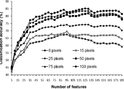
accuracy and that obtained from the use of all 65 features was 5.00%, a difference that was significant at the 0.05 level of significance (Table I).
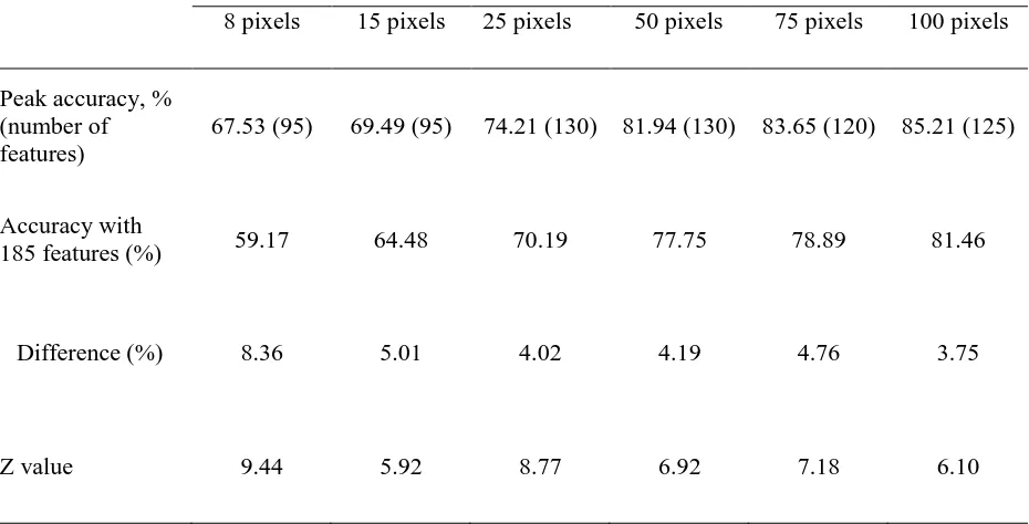
Similar general trends to those found with the analysis of the DIAS data were observed with the results of the analyses of the AVIRIS data set (Fig. 2). Critically, classification accuracy was observed to decline with the addition of features. Moreover, with this data set, a statistically significant (at 0.05 level) decline in accuracy with the addition of features was observed for all training set sizes (Table II). The largest difference between the peak accuracy and that obtained from the use of all 185 features was 8.36%.
Insert Fig. 1- 2 here
Having established that the accuracy of classification by a SVM is sensitive to the number of features used, the four different feature selection methods were applied to the DIAS data in order to evaluate the sensitivity of SVM classification to different types of feature selection method. The aim was not to define an optimal feature selection but to provide insight into the sensitivity of the SVM classification to the method used.
The classifications derived after application of the four feature selection methods varied in accuracy. Unlike the previous analyses, features were added individually to classifications in the order suggested by the feature selection analysis. To focus on key trends, Table III shows the accuracy derived without feature selection and the accuracy that was of closest magnitude after the application of each of the feature selection methods. Critically, the table also identifies the number of features used to derive the classification accuracy closest to that derived when no feature selection was undertaken. Irrespective of feature selection algorithm employed, the results suggest that a small subset of selected features (≤ 12) would be sufficient to achieve comparable accuracy with the small training sets comprising 8, 15 and 25 pixels per-class. In comparison, the training sets with 50, 75 and 100 pixels per-class requires a larger subset of selected features to achieve the comparable classification accuracy to that derived from the full dataset (and the accuracy values were also of a higher magnitude).
Insert Table III here
It was also evident that the specific features selected by the different methods varied. Table IV identifies the selected features that provided the classification of comparable accuracy to that derived from the full (65 features) dataset. It was evident that a dissimilar feature list was obtained from analyses based on training sets of differing size, with at most only three common features observed with any one feature selection method. The outputs of the feature selection methods was, therefore, a function of the training set size. Moreover, the lack of commonalities in features selected with different training set sizes also confirms that the best set of features selected by a nonexhaustive search need not to contain the best feature or a set of best features from the full feature space [67].
Insert Table IV here
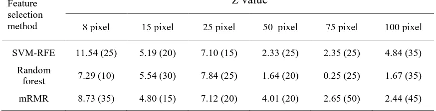
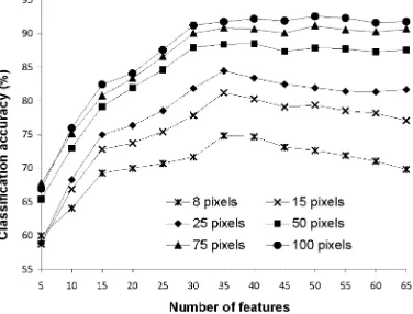
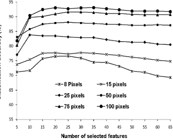
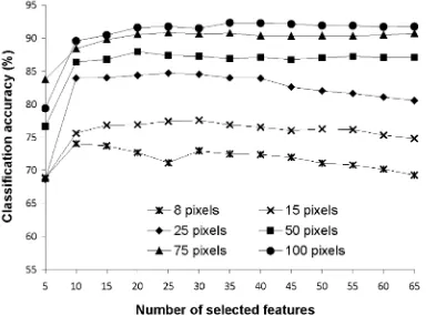
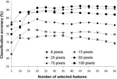
For comparison against the results given in Fig. 1, Fig. 3-5 show the relationship between classification accuracy and number of selected features using three of the feature selection methods. The CFS based feature selection method was excluded from this analysis as this approach does not provide a ranked list of the features. For purpose of comparability with Fig. 1 the features have been added in groups of 5 (in order of discriminating ability). The statistical significance of the difference in accuracy between the peak accuracy value and that derived with the use of the full feature set for each classification summarised in Fig. 3-5 was evaluated with a McNemar test. The derived Z-values are provided in Table V which suggests a similar trend as achieved with earlier
combination of features (Fig. 1) using the training sample size of 8, 15, and 25 pixels per class. It was evident, however, that the peak accuracy was derived with a smaller number of features as in this case features were added in order of discriminating power.
The results highlight that a statistically significant negative impact of feature set size on classification accuracy was observed when a small training sample was used; confirming the results of the McNemar test for a significant difference. Although this in itself points to a dependency of SVM classification on the dimensionality of the data set and highlights a positive role for feature selection analysis the latter has other advantages and the results suggest feature selection may be valuable even when a large training sample was available. Note, for example, that in all series of analyses (Fig. 1 and Fig. 3-5) when the largest training sample was used (100 cases per-class) the accuracy was largely maintained when the number of features is reduced from the full (65 features) to small sub-set; only at a very small number of features did classification accuracy decline markedly. This similarity in accuracy values shows that the positive benefits of feature selection (e.g. reduced data storage and processing requirements) may be achieved without significant negative effect on classification accuracy. The latter is evident in the results of the non-inferiority testing summarised in Tables VI-VIII. Critically, the accuracy of classifications derived with the use of relatively small training sets was not statistically inferior to the peak accuracy derived from the use of a larger feature set size.
V. CONCLUSIONS
manifested in the results was limited through experimental design, notably through the use of a large training set. The results presented in this paper show that the accuracy of classification by a SVM can be significantly reduced by the addition of features and that the effect is most apparent with small training sets. With the AVIRIS data set, a significant reduction in accuracy with the addition of features was observed at all training set sizes evaluated. With the DIAS data set, a statistically significant decline in accuracy was also observed for small training sets (≤25 cases per-class). However, even with a large training sample using DAIS dataset, feature selection may have a positive role, providing a reduced data set that may be used to yield a classification of similar accuracy to that derived from use of a much larger feature set. As the accuracy of SVM classification was dependent on the dimensionality of the data set and the size of the training set it may, therefore, be beneficial to undertake a feature selection analysis prior to a classification analysis. The results, however, also highlight that the choice of feature selection methods may be important. For example, the results derived from analyses with four different feature selection methods show that the number of features selected varied greatly.
Acknowledgements
REFERENCES
[1] C.-I Chang, Hyperspectral Data Exploitation: Theory and Applications. New Jersey: John Wiley and Sons, 2007.
[2] J. B. Campbell, Introduction to Remote Sensing. Third edition, New York: The
Guilford press, 2002.
[3] J. A. Benediktsson and J. R. Sveinsson, “Feature extraction for multisource data classification with artificial, neural networks,” International Journal of Remote Sensing, vol. 18, no. 4, pp. 727-740, March 1997.
[4] P. Zhong, P. Zhang, and R. Wang, “Dynamic learning of SMLR for feature selection and classification of hyperspectral data,” IEEE Geoscience and Remote Sensing Letters, vol. 5, no. 2, pp. 280-284, April 2008.
[5] B. M. Shahshahani and D. A. Landgrebe, “The effect of unlabeled samples in reducing the small sample size problem and mitigating the Hughes phenomenon,” IEEE Transactions on Geoscience and Remote Sensing, vol. 32, no. 5,
pp.1087-1095, Sept.1994.
[6] S. Tadjudin and D.A. Landgrebe, “Covariance estimation with limited training samples,” IEEE Transactions on Geoscience and Remote Sensing, Vol. 37, no. 4, pp. 2113-2118, July 1999.
[7] M. Chi, R. Feng, and L.Bruzzone, “Classification of hyperspectral remote-sensing data with primal SVM for small-sized training dataset problem,” Advances in Space Research, vol. 41, no. 4, pp. 1793–1799, 2008.
[9] S. Lu, K. Oki, Y. Shimizu, and K. Omasa, “Comparison between several feature extraction/classification methods for mapping complicated agricultural land use patches using airborne hyperspectral data,” International Journal of Remote Sensing, vol. 28, no. 5, pp. 963-984, Jan. 2007.
[10] S. Tadjudin and D. A. Landgrebe, “A decision tree classifier design for high-dimensional data with limited training samples,” IEEE Geoscience and Remote Sensing Symposium, Vol. 1, pp. 790-792, 27-31 May 1996.
[11] M. Chi and L. Bruzzone, “A semilabeled-sample-driven bagging technique for ill-posed classification problems,” IEEE Geosciences Remote Sensing Letters, vol. 2, no. 1, pp. 69–73, January 2005.
[12] P. Mantero, G. Moser and S.B. Serpico, “Partially supervised classification of remote sensing images through SVM-based probability density estimation,” IEEE Transactions on Geoscience and Remote Sensing, vol. 43, no. 3, pp. 559–570,
March 2005.
[13] G. M. Foody and A. Mathur, “Toward intelligent training of supervised image classifications: directing training data acquisition for SVM classification,” Remote Sensing of Environment, vol. 93, no. 1-2, pp. 107–117, Oct. 2004.
[14] V. N. Vapnik, The Nature of Statistical Learning Theory. New York: Springer-Verlag, 1995.
[15] C. Cortes and V. N. Vapnik, “Support vector networks,” Machine Learning, vol. 20, no. 3, pp. 273-297, Sept. 1995.
[17] D. M. J. Tax, D. de Ridder, and R.P.W. Duin, “Support vector classifiers: A first look,” in: H.E. Bal, H. Corporaal, P.P. Jonker, J.F.M. Tonino (eds.), Proceedings of 3rd Annual Conference of the Advanced School for Computing and Imaging
(Heijen, NL, June 2-4), ASCI, Delft, pp. 253-258, 1997.
[18] J. A. Gualtieri, “The support vector machine (SVM) algorithm for supervised classification of hyperspectral remote sensing data,” In G. Camps-Valls and L. Bruzzone (eds) Kernel Methods for Remote Sensing Data Analysis, Wiley, Chichester, in press, 2009.
[19] M. Pal, and P. M. Mather, “Assessment of the effectiveness of support vector machines for hyperspectral data,” Future Generation Computer Systems, vol. 20, no. 7, pp. 1215–1225, October 2004.
[20] M. Pal and P. M. Mather, “Some issue in classification of DAIS hyperspectral data,” International Journal of Remote Sensing, vol. 27, no. 14, pp. 2895–2916, July 2006.
[21] F. Melgani and L. Bruzzone, “Classification of hyperspectral remote sensing images with support vector machines,” IEEE Transaction of Geoscience and Remote Sensing, vol. 42, no. 8, pp. 1778-1790, August 2004.
[22] I. Guyon, J. Weston, S. Barnhill, and V. N. Vapnik, “Gene selection for cancer classification using support vector machines,” Machine Learning, vol. 46, no. 1-3, pp. 389-422, Jan. 2002.
[23] A. Gidudu and H. Ruther, “Comparison of feature selection techniques for SVM classification,” In 10th Intl. Symposium on Physical Measurements and Spectral Signatures in Remote Sensing (eds M.E. Schaepman, S. Liang, N.E. Groot, and M.
Information Sciences, Vol. XXXVI, Part 7/C50, p. 258-263, 2007. ISPRS, Davos (CH). ISSN 1682-1777.
[24] H. Liu, “Evolving feature selection,” IEEE Intelligent Systems, vol. 20, pp. 64-76, November 2005.
[25] H. Liu and H. Motoda, Feature Extraction, Construction and Selection: A Data Mining Perspective. Massachusetts: Kluwer Academic Publishers, 1998.
[26] P. M. Mather, Computer Processing of Remotely-Sensed Images: An Introduction. Third Edition, Chichester: John Wiley and Sons, 2004.
[27] R. Kohavi and G.H. John, “Wrappers for feature subset selection,” Artificial Intelligence, vol. 97, no. 1-2, pp. 273-324, March 1997.
[28] I. Guyon and A. Elisseeff, “An introduction to variable and feature selection,” Journal of Machine Learning Research, vol. 3, pp. 1157-1182, March 2003.
[29] M. Dash and H. Liu, “Feature selection for classification,” Intelligent Data Analysis: An International Journal, vol.1, no. 3, pp.131-156, 1997.
[30] A. Jain and D. Zongker, “Feature selection: evaluation, application, and small sample performance,” IEEE Transactions on Pattern Analysis and Machine Intelligence, vol. 19, no. 2, pp. 153-158, February 1997.
[31] T. Kavzoglu and P. M. Mather, “The role of feature selection in artificial neural network applications,” International Journal of Remote Sensing, vol. 23, no 15, pp. 2787–2803, Aug. 2002.
[33] M. Pal, “Support vector machine-based feature selection for land cover classification: a case study with DAIS hyperspectral data,” International Journal of Remote Sensing, vol. 27, no. 14, pp. 2877–2894, July 2006.
[34] J. Loughrey and P. Cunningham, “Overfitting in wrapper-based feature subset selection: the harder you try the worse it gets,” Research and Development in
Intelligent Systems XXI (Max Bramer, Frans Coenen and Tony Allen, eds.),
Springer, London, pp. 33-43, 2004.
[35] G.H. Halldorsson, J.A. Benediktsson, J.R. Sveinsson, “Source based feature extraction for support vector machines in hyperspectral classification,” IEEE Geoscience and Remote Sensing Symposium, vol. 1, pp. 536-539, 20-24 Sept.
2004.
[36] O. Barzilay and V. L. Brailovsky, “On domain knowledge and feature selection using a support vector machine,” Pattern recognition Letters, vol. 20, no. 5, pp. 475-484, May 1999.
[37] A. Navot, R. Gilad-Bachrach, Y. Navot, and N. Tishby, “Is feature selection still necessary?” Lecture notes in computer science, Berlin Heidelberg: Springer-Verlag, vol. 3940, pp. 127-138, 2006.
[38] Y. Bengio, O. Delalleau, and N. Le Roux, “The curse of highly variable functions for local kernel machines,” in: Advances in Neural Information Processing Systems, MIT Press, vol.18, pp. 107-114, 2006.
[40] B. Scholkopf, S. Mika, C.J.C. Burges, P. Knirsch, K.R. Muller, G. Ratsch, and A.J. Smola, “Input space versus feature space in kernel-based methods,” IEEE Transactions on Neural Networks, vol.10, no. 5, pp.1000-1017, September 1999.
[41] S. Geman, E. Bienenstock and R. Doursat, “Neural networks and the bias/variance dilemma,” Neural Computation, vol. 4, no. 1, pp. 1–58, Jan. 1992.
[42] J. L. Fleiss, B. Levin, and M. C. Paik, Statistical Methods for Rates & Proportions. Third edition, New York: Wiley-Interscience, 2003
[43] G. M. Foody, “Classification accuracy comparison: hypothesis tests and the use of confidence intervals in evaluations of difference, equivalence and non-inferiority,” Remote Sensing of Environment, vol. 113, pp. 1658-1663, 2009.
[44] B. Boser, I. Guyon, and V. N. Vapnik, “A training algorithm for optimal margin classifiers,” Proceedings of 5th
Annual Workshop on Computer Learning Theory,
Pittsburgh, PA: ACM, pp.144-152, 1992.
[45] N. Cristianini, and J. Shawe-Taylor, An Introduction to Support Vector Machines and other Kernel-based Learning Methods. Cambridge, UK: Cambridge
University Press, 2000.
[46] G.M. Foody and A. Mathur, “A relative evaluation of multiclass image classification by support vector machines,” IEEE Transaction of Geoscience and Remote Sensing, vol. 42, no. 6, pp. 1335-1343, June 2004.
[47] G. Camps-Valls and L. Bruzzone, Kernel Methods for Remote Sensing Data Analysis (eds), Wiley, Chichester, in press.
[49] Aviris NW Indiana‟s Indian Pines, 1992, data set [online]. Available Online: ftp://ftp.ecn.purdue.edu/biehl/MultiSpec/92AV3C.lan (original files) and ftp://ftp.ecn.purdue.edu/biehl/PC_MultiSpec/ThyFiles.zip (ground truth).
[50] G.M. Foody and M.K. Arora, “An evaluation of some factors affecting the accuracy of classification by an artificial neural network,” International Journal of Remote Sensing, vol. 18, no. 4, pp. 799–810, March 1997.
[51] G. M. Foody, A. Mathur, C. Sanchez-Hernandez, D. S. Boyd, “Training set size requirements for the classification of a specific class,” Remote Sensing of Environment, vol. 104, no. 1, pp. 1-14, Sept. 2006.
[52] M. Pal and P.M. Mather, “An assessment of the effectiveness of decision tree methods for land cover classification,” Remote Sensing of Environment, vol. 86, no. 4, pp. 554–565, October 2003.
[53] T. G. Van Niel, T. R. McVicar, and B. Datt, “On the relationship between training sample size and data dimensionality of broadband multi-temporal classification,” Remote Sensing of Environment, vol. 98, no. 4, pp. 468−480, October 2005.
[54] T.G. Dietterich, “Approximate statistical tests for comparing supervised classification learning algorithms,” Neural Computation, vol.10, no. 7, pp. 1895– 1923, October 1998.
[55] G.M. Foody, “Thematic map comparison: evaluating the statistical significance of differences in classification accuracy,” Photogrammetric Engineering and Remote Sensing, vol.70, no. 5, pp.627–633, May 2004.
[57] M. A. Hall and L. A. Smith, “Feature subset selection: a correlation based filter approach,” International Conference on Neural Information Processing and Intelligent Information Systems, Springer, pp. 855-858, 1997.
[58] W.H. Press, Numerical Recipes in C. Cambridge: University Press, 1988.
[59] H. Peng, F. Long and C. Ding, “Feature selection based on mutual information: criteria of max-dependency, max-relevance, and min-redundancy,” IEEE Transactions on Pattern Analysis and Machine Intelligence, vol. 27, no. 8, pp.
1226-1238, August 2005.
[60] L. Breiman, “Random forests,” Machine Learning, vol. 45, no. 1, pp. 5–32, October 2001.
[61] L. Breiman, “Bagging predictors,” Machine Learning, vol. 24, no. 2, pp. 123-140, August 1996.
[62] R. Díaz-Uriarte and S.A. de Andrés, “Gene selection and classification of microarray data using random forest,” BMC Bioinformatics, 7:3, 2006.
[63] C.-W. Hsu, and C.-J. Lin, “A comparison of methods for multi-class support vector machines,” IEEE Transactions on Neural Networks, vol. 13, no. 2, pp. 415-425, March 2002.
[64] M. Pal, “Multiclass approaches for support vector machine based land cover classification,” 8th Annual International conference, Map India, http://www.mapindia.org/2005/papers/pdf/54.pdf (accessed on 12/11/2008), 2005. [65] S. Knerr, L. Personnaz and G. Dreyfus, “Single-layer learning revisited: A stepwise
[66] M. Pal, “Margin based feature selection for hyperspectral data,” International Journal of Applied Earth Observations and Geoinformation, vol. 11, no. 3, pp.
212-220, June 2009.
[67] T. M. Cover, “The best two independent measurements are not the two best,” IEEE Transactions on Systems, Man, and Cybernetics, vol. SMC-4, pp.116-117, January
TABLE CAPTIONS
Table I. Difference between peak accuracy and that derived from the use of all 65 features of DAIS dataset for the results summarised in Fig. 1. The Z value stated was derived from the McNemar test. For the one-sided test adopted a difference is significant at the 0.05 level if Z>1.64.
Table II. Difference between peak accuracy and that derived from the use of all 185 features of AVIRIS dataset for the results summarised in Fig. 2. The Z value stated was derived from the McNemar test. For the one-sided test adopted a difference is significant at the 0.05 level if Z>1.64.
Table III. Results of the application of the 4 feature selection methods using DAIS dataset highlighting characteristics of the classification based on each training set size that was of most comparable accuracy to that derived without feature selection.
Table IV. Selected features with different data sets and the number of common features selected by various approaches using DAIS dataset.
Table V. Summary of the test for the difference in accuracy between the peak accuracy and that derived from the use of the full feature set using DAIS dataset. Values in bracket gives the number of features providing peak classification accuracy, shown in Fig. 2-4. The Z value stated was derived from the McNemar test. For the one-sided test adopted a difference is significant at the 0.05 level if Z>1.64.
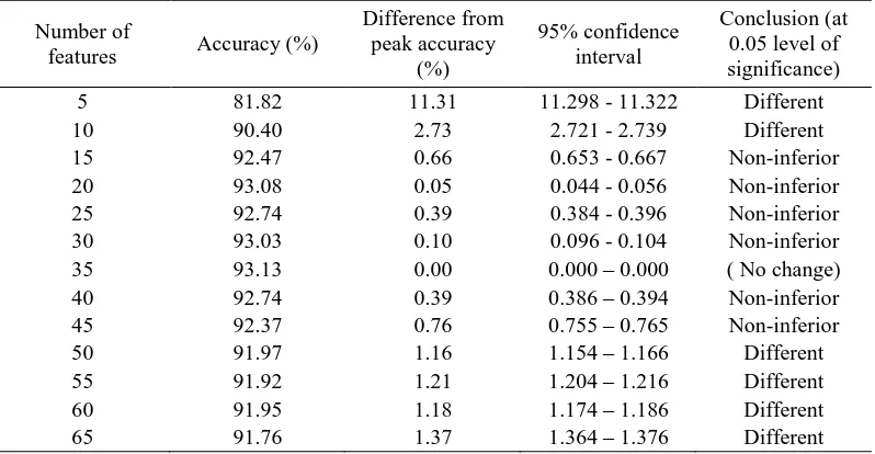
Table VI. Difference and non-inferiority test results based on 95% confidence interval on the estimated difference in accuracy from the peak value for feature sets selected with the SVM-RFE using DAIS dataset; based on training set of 100 cases per-class with peak accuracy of 93.13% with 35 features.
Table VII. Difference and non-inferiority test results based on 95% confidence interval on the estimated difference in accuracy from the peak value for feature sets selected with the random forest using DAIS dataset; based on training set of 100 cases per-class with peak accuracy of 92.34% with 35 features.
Table I.
Training set size per class
8 pixels 15 pixels 25 pixels 50 pixels 75 pixels 100 pixels
Peak accuracy, % (number of features)
74.79 (35) 81.21 (35) 84.45 (35) 88.47 (40) 91.13 (50) 92.53 (50)
Accuracy with 65
features (%) 69.79 77.05 81.66 87.58 90.63 91.76
Difference (%) 5.00 4.16 2.79 0.89 0.50 0.77
Table II.
Training set size per class
8 pixels 15 pixels 25 pixels 50 pixels 75 pixels 100 pixels
Peak accuracy, % (number of features)
67.53 (95) 69.49 (95) 74.21 (130) 81.94 (130) 83.65 (120) 85.21 (125)
Accuracy with
185 features (%) 59.17 64.48 70.19 77.75 78.89 81.46
Difference (%) 8.36 5.01 4.02 4.19 4.76 3.75
Table III. Feature
selection Method
Training set size per class
8 pixels 15 pixels 25 pixels 50 pixels 75 pixels 100 pixels
Accuracy (%) Feature size Accuracy (%) Feature size Accuracy (%) Feature size Accuracy (%) Feature size Accuracy (%) Feature size Accuracy (%) Feature size None
69.29 65 74.82 65 80.58 65 87.10 65 90.71 65 91.76 65
SVM-RFE 69.84 4 75.39 10 81.68 7 87.45 15 90.87 16 91.89 13
mRMR
69.71 8 76.34 11 81.02 12 87.13 13 90.87 42 91.84 37
CFS
69.50 4 75.82 7 82.18 8 87.11 12 91.32 14 91.84 17
Random
Table IV. Feature
selection approach
Training set size per class Number
of common
features 8 pixels 15 pixels 25 pixel 50 pixel 75 pixels 100 pixels
SVM-RFE 1,4,35,53
1,4,6,27,32, 36,37,50,51, 57 1,3,4,26,32, 37,42 1,2,3,4,18, 26,27,31,32, 36,37,46,48, 52,56 1,2,3,4,5,26, 27,30,31,32, 34,36,37,40, 52,56 1,2,3,21,26, 27,30,34,36,
37,51,52,56 1
mRMR 10,15,16,17, 24,25,49,56 9,16,22,24, 25,26,32,48, 49,50,65 9,15,22,24, 25,26,29,31, 32,48,49,51 8,21,22,23, 24,25,26,27, 28,30,49,50, 65 2,3,6,7,8,9, 10,12,13,14, 15,16,17,18, 19,20,21,22, 23,24,25,26, 27,28,29,30, 31,32,36,37, 38,41,47,48, 49,50,51,52, 53,63,64,65 6,7,8,9,12, 13,14,15,16, 17,18,19,20, 21,22,23,24, 25,26,27,28, 29,30,31,32, 33,38,41,47, 48,49,50,51, 52,53,63,65 3
Table V. Feature
selection method
Z value
8 pixel 15 pixel 25 pixel 50 pixel 75 pixel 100 pixel
SVM-RFE 11.54 (25) 5.19 (20) 7.10 (15) 2.33 (25) 2.35 (25) 4.84 (35)
Random
forest 7.29 (10) 5.54 (30) 7.84 (25) 1.64 (20) 0.25 (25) 1.67 (35)
Table VI. Number of
[image:38.595.100.499.148.355.2]features Accuracy (%)
Difference from peak accuracy
(%)
95% confidence interval
Conclusion (at 0.05 level of significance) 5 81.82 11.31 11.298 - 11.322 Different
10 90.40 2.73 2.721 - 2.739 Different
15 92.47 0.66 0.653 - 0.667 Non-inferior 20 93.08 0.05 0.044 - 0.056 Non-inferior 25 92.74 0.39 0.384 - 0.396 Non-inferior 30 93.03 0.10 0.096 - 0.104 Non-inferior 35 93.13 0.00 0.000 – 0.000 ( No change) 40 92.74 0.39 0.386 – 0.394 Non-inferior 45 92.37 0.76 0.755 – 0.765 Non-inferior
50 91.97 1.16 1.154 – 1.166 Different
55 91.92 1.21 1.204 – 1.216 Different
60 91.95 1.18 1.174 – 1.186 Different
Table VII. Number of
features Accuracy (%)
Difference from peak accuracy
(%)
95% confidence interval
Conclusion (at 0.05 level of significance) 5 79.37 12.97 12.958 – 12.982 Different
10 89.58 2.76 2.751 - 2.769 Different
15 90.47 1.87 1.862 – 1.878 Different
20 91.61 0.73 0.724 – 0.736 Non-inferior 25 91.76 0.58 0.573 – 0.587 Non-inferior 30 91.50 0.84 0.835 – 0.845 Non-inferior
35 92.34 0.00 0.000 – 0.000 (No change)
Table VIII. Number of
features Accuracy (%)
Difference from peak accuracy
(%)
95% confidence interval
Conclusion (at 0.05 level of significance)
5 80.97 11.48 11.468 – 11.492 Different
10 88.5 3.95 3.940 – 3.960 Different
15 88.82 3.63 3.620 – 3.640 Different
20 91.24 1.21 1.202 – 1.218 Different
25 91.58 0.87 0.862 – 0.878 Non-inferior
30 91.03 1.42 1.413 – 1.427 Different
35 91.53 0.92 0.914 – 0.926 Non-inferior 40 92.16 0.29 0.286 – 0.294 Non-inferior
45 92.45 0.00 0.000 – 0.000 (No change)