A Comparative Study on the Control of Quadcopter UAVs by using
Singleton and Non-Singleton Fuzzy Logic Controllers
Changhong Fu
1,2, Andriy Sarabakha
1,2, Erdal Kayacan
1Christian Wagner
3, Robert John
3and Jonathan M. Garibaldi
3Abstract— Fuzzy logic controllers (FLCs) have extensively
been used for the autonomous control and guidance of un-manned aerial vehicles (UAVs) due to their capability of han-dling uncertainties and delivering adequate control without the need for a precise, mathematical system model which is often either unavailable or highly costly to develop. Despite the fact that non-singleton FLCs (NSFLCs) have shown more promising performance in several applications when compared to their sin-gleton counterparts (SFLCs), most of UAV applications are still realized by using SFLCs. In this paper, we explore the potential of both standard and the recently introduced centroid based NSFLCs, i.e., Sta-NSFLC and Cen-NSFLC, for the control of a quadcopter UAV under various input noise conditions using different levels of fuzzifier, and a comparative study has been conducted using the three aforementioned FLCs. We present a series of simulation-based experiments, the simulation results show that the control performances of NSFLCs are better than those of SFLC, and the Cen-NSFLC outperforms the Sta-NSFLC especially under highly noisy conditions.
I. INTRODUCTION
Unmanned aerial vehicles (UAVs) have been widely uti-lized in a variety of civilian applications to save time, money and even lives, e.g., disaster rescue [1], target tracking [2], orchard monitoring [3], wildlife protection [4], infrastructure inspection [5] and 3D environment reconstruction [6]. Most of the time, to achieve fully autonomous flight in these UAV applications, classical controllers, e.g. proportional-integral-derivative (PID) [7], linear quadratic regulators (LQRs) [8] or sliding mode control (SMC) [9], have been utilized. There is no doubt that these well-known control algorithms are very successful when a precise mathematical model of the system is obtained and no significant internal or external uncertain-ties exist. On the other hand, modelling of complex dynamics systems is a tedious, costly and time consuming task [10]. Unfortunately, lack of modeling, uncertainty, inaccuracy in the sensors, approximation and incompleteness problems are inevitable in a typical UAV application. For instance, considerable uncertainties exist in the different types of
1Changhong Fu, Andriy Sarabakha and Erdal Kayacan
are with School of Mechanical and Aerospace Engineering, Nanyang Technological University (NTU), 50 Nanyang Avenue, Singapore 639798. Email: [email protected], [email protected], [email protected]
2Changhong Fu and Andriy Sarabakha are with ST Engineering-NTU
Corp Laboratory, 50 Nanyang Avenue, Singapore 639798
3Christian Wagner, Robert John and Jonathan M. Garibaldi are with Lab
for Uncertainty in Data and Decision Making (LUCID), School of Computer Science, University of Nottingham, Nottingham, United Kingdom. Email: [email protected], [email protected],
onboard UAV sensors, e.g., global positioning system (GPS), monocular/stereo cameras, laser range finders (LRFs) and inertial measurement units (IMUs).
In this study, we explore the potential of both standard and recently introduced centroid-based variants of non-singleton FLCs (NSFLCs) to address uncertainty affecting the inputs of quadcopter UAV control. Although there are a number of FLC applications for navigating a quadcopter UAV in litera-ture, e.g., [11], most of these are SFLCs, which focus on high level navigation, rather than exploring the effect of various levels of input uncertainty on the control performance. On the other hand, it is reported in literature that NSFLCs give more promising results when compared to their singleton counterparts for non-linear servo system [12], chaotic time series prediction [13], etc. Both FLCs use the same fuzzy rule base, inference engine and defuzzifier. However, in the NSFLC, there is a different fuzzifier which treats the inputs as fuzzy sets (FSs). In this paper, we employ Gaussian input fuzzy sets with different standard deviations to capture different levels of uncertainty.
Another motivation of this investigation is to compare and contrast the performances of different types of NSFLCs, in addition to the standard NSFLC (Sta-NSFLC), centroid NSFLC (Cen-NSFLC) is also used. In spite of Sta-NSFLC is capable of handling uncertainties by capturing them from inputs, the adopted prefiltering approach in the Sta-NSFLC does not offer a fine-grained uncertainty information track-ing, i.e., the prefilter is not highly sensitive to the shape of the input of FSs, leading to significant loss of information regarding the intersection of input and antecedent models. Therefore, an alternative type of the NSFLC initially de-veloped in [14], [15], i.e.,Cen-NSFLC, has been dede-veloped for controlling the quadcopter UAV. In [14], [15], the novel approach to NSFLCs showed promising results in the context of time-series prediction with different levels of injected uncertainty. The aim of the work discussed in this paper is to move beyond simulated levels of uncertainty to real-world uncertainty affecting real world sensors.
Finally, some conclusions are drawn from this study and possible future works are also presented in Section V.
II. QUADCOPTERUAV DYNAMICS
In this section, we introduce the configuration, equations of motion as well low level velocity control of the quad-copter.
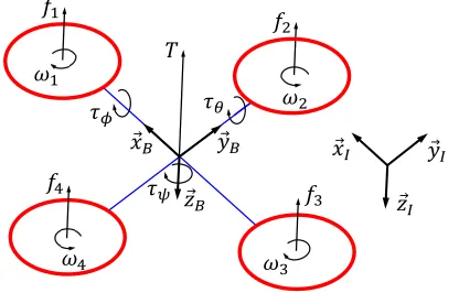
A. Configuration definition
Let the world fixed inertial reference frame be{~xI, ~yI, ~zI}
and the body frame be{~xB, ~yB, ~zB}. The origin of the body
frame is located at the center of mass of the quadcopter. The axes~xB and~yBlie in the plane defined by the centres of the
four rotors and respectively point toward motor 1 and motor 2, as illustrated in Fig. 1. The axis~zI points downward, as
well as axis~zBwhich is opposite to the direction of the total
thrust.
𝜔2
𝜔3
𝜔4
𝜔1
𝑓1
𝑓4 𝑓
3
𝑓2
𝜏𝜙
𝜏𝜓
𝜏𝜃
𝑥 𝐵 𝑦 𝐵
𝑧 𝐵
𝑦 𝐼
𝑥 𝐼
𝑧 𝐼
[image:2.612.72.280.257.390.2]𝑇
Fig. 1: Quadrotor model with reference frames.
The four propellers generate four forces (f1, f2, f3 and
f4), directed along the axis of rotation~zB and with module
proportional to the speed of rotation, and four torques (τ1,τ2,
τ3andτ4), around the axis of rotation~zB and with module
proportional to the speed of rotation [16]. The forces and torques are proportional to the square of the angular speed of the propeller:
fi=bω2i, τi=dlω2i, i= 1, . . . ,4, (1)
wherebis the propeller thrust coefficient, dis the propeller drag coefficient and ωi is the rotational speed of the ith
propeller.
The quadrotor control vector uis considered as follows:
u=
T τφ τθ τψ
T
, (2)
whereT is the total thrust and acts along~zB axis, whereas
τφ,τθandτψare the moments acting around~xB,~yBand~zB
axes, respectively. Under these considerations, the relation betweenuandωi,i= 1, . . . ,4, becomes [17]:
T =f1+f2+f3+f4 (3)
τφ=l(−f2+f4) (4)
τθ=l(f1−f3) (5)
τψ=−τ1+τ2−τ3+τ4, (6)
wherel is the arm length.
The absolute position of a quadcopter (3 DOF) is described by the three Cartesian coordinates (x,yandz) of its center of mass in the world frame and its attitude by the three Euler’s angles (φ, θ and ψ). These three angles are respectively called roll (−π
2 < φ < π
2), pitch (− π 2 < θ <
π
2) and yaw
(0≤ψ <2π).
The time derivative of the position (x,y,z) is given by
V= ˙
x y˙ z˙T =
u v wT
, (7)
whereVis the absolute velocity of the quadcopter’s center of mass expressed with respect to the world fixed inertial reference frame. Let VB ∈ R3 be the absolute velocity of
the quadcopter expressed in the body fixed reference frame. So,VandVB are related by
V=RVB, (8)
whereR∈SO(3)is the rotation matrix from the body frame to the world frame:
R=
cψcθ cψsφsθ−cφsψ sφsψ+cφcψsθ
cθsψ cφcψ+sφsψsθ cφsψsθ−cψsφ
−sθ cθsφ cφcθ
, (9)
wherecθ andsθ denote respectivelycosθ andsinθ.
Similarly, the time derivative of the angles (φ, θ, ψ) give the angular velocities:
ω=˙
φ θ˙ ψ˙T
, (10)
and the angular velocities expressed in the body frame are
ωB=
p q rT. (11)
The relation betweenω andωB is given by
ω=TωB, (12)
in whichT is the transformation matrix given by
T=
1 sinφtanθ cosφtanθ
0 cosφ −sinφ
0 sinφsecθ cosφsecθ
. (13)
B. Equations of motion of the quadrotor
Using the Newton-Euler equations about the center of mass, the dynamic equations for the quadcopter are [18]:
mV˙ =Fe (14)
Iω˙B =−ωB×IωB+τe, (15)
wheremis the mass and Iis the inertia matrix given by
I=
Ix 0 0
0 Iy 0
0 0 Iz
andFeis the vector of external forces and τeis the vector
of external torques. Some calculations yield the following form for these two vectors
Fe=
−(cosφsinθcosψ+ sinφsinψ)T −(cosφsinθsinψ−sinφcosψ)T
−cosφcosθT +mg
(17)
τe=
τφ τθ τψ
, (18)
in which g is the gravity acceleration (g= 9.81m/s2).
Using dynamic and kinematic differential equations (8), (12), (15) and (18), the quadcopter model is obtained [19]
˙
x=u
˙
y=v
˙
z=w
˙
φ=p+ sinφtanθq+ cosφtanθr
˙
θ= cosφq−sinφr
˙
ψ= sincosφθq+coscosφθr
˙
u=−1
m(cosφcosψsinθ+ sinφsinψ)T
˙
v=−1
m(cosφsinψsinθ−cosψsinφ)T
˙
w=−1
mcosφcosθT+g
˙
p=Iy−Iz
Ix qr+
1 Ixτφ
˙
q= Iz−Ix
Iy pr+
1 Iyτθ
˙
r= Ix−Iy
Iz pq+
1 Izτψ.
(19)
Hence, the quadrotor’s state xis
x= x y z φ θ ψ u v w p q r T.
(20)
C. Low level velocity control
After the quadcopter dynamic model is identified, the low level velocity controller is designed. The control law is based on a proportional-derivative (PD) algorithm. The inputs to the PD-based attitude controller are the desired linear velocity
V∗=
u∗ v∗ w∗T
(21)
and the desired angular velocityψ˙∗ around the~zI axes, and
the output is defined in (2).
III. BACKGROUND OFSFLCANDNSFLC
In this section, we present a brief background overview of the SFLC, Sta-NSFLC and Cen-NSFLC.
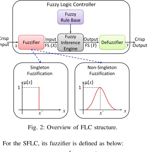
[image:3.612.77.297.104.179.2]A. Structure of FLC
Figure 2 shows the general structure of a FLC. The fuzzy rule base (purple block), inference engine (grey block) and defuzzifier (green block) are the same in both NSFLC and SFLC. However, the difference between SFLC and NSFLC is the handling of the crisp inputs in the fuzzifier (red block). The NSFLC maps a given crisp input to a fuzzy input set,
rather than to a fuzzy singleton - as is the case in the SFLC, i.e. the fuzzifier of SFLC does not model any vagueness in the input. Fuzzifier Fuzzy Inference Engine Fuzzy Rule Base Defuzzifier Crisp Input Crisp Output x y Output FS (Y) Input FS (X)
Fuzzy Logic Controller
Singleton Fuzzification
1 μ(x)
x´ x
Non-Singleton Fuzzification
1 μ(x)
[image:3.612.319.558.106.350.2]x´ x
Fig. 2: Overview of FLC structure.
For the SFLC, its fuzzifier is defined as below:
µX(xi) =
(
1, xi=x
0
i
0, xi6=x
0
i.
(22)
For the NSFLC, the Gaussian distribution is selected for its fuzzifier in our case, i.e.:
µX(xi) = exp
−(x
i−x0i)2
2σ2 F
, (23)
wherex0i is the crisp value of the input and the mean value of the fuzzy set, and σF is the spread of this set. Larger
values of the spread imply that more noise is anticipated to exist in the input data.
In the literature, standard NSFLCs have been defined for both type-1 and type-2 FLCs. However, we limit ourselves to 1 non-singleton 1 FLC in this work, i.e. type-1 input membership functions (MFs) are adopted for type-type-1 FLCs. The general mapping between the inputs and outputs of the FLCs, as the input setX and output setY are shown in Fig. 2, is comprehensively introduced in [20]. This paper will not repeat the details of how the comprehensive formula for the mapping is derived. Since the prefiltering module of the NSFLC is the key to handling the input uncertainties, as shown in Fig. 3, we introduce the details of this prefiltering module below.
Specifically, the inference engine of a NSFLC can be considered as a prefilter module embedded to a SFLC inference engine. The prefilter module converts the crisp input in combination with the uncertain input set to a representive numberical value xmax. The handling of the
Prefilter Inference μC(y)
μX(x) xmax μY(y)
Fig. 3: Prefiltering of the input FS to a NSFLC.
nature of the prefiltering stage for both standard and centroid-based [14], [15] NSFLCs.
[image:4.612.57.289.52.122.2]B. Prefiltering module in Sta-NSFLC
Figure 4 provides an example of a input, single-rule and single-output discrete standard NSFLC has been considered, and the Mamdani implication is utilized.
1 μ(x)
xmax
x
1 μ(y)
y
μx(x) μA(x)
μx(x) μA(x)
μC(y)
[image:4.612.332.540.219.363.2]μY(y)
Fig. 4: Example of the calculation from input (X), antecedent (A) and consequent (C) fuzzy sets to output (Y). (Adapted from [14], [15])
Let x and y be the members of the input FS (X) and output FS (Y), and A and C are two FSs representing an antecedent and a consequent. The only rule is defined as:
IFxisATHENy isC. (24) TheµX(x),µA(x),µC(y)andµY(y)are the MFs ofX,
A, C and Y, respectively. Note that we only consider the Gaussian MFs in this work, then the input-output mapping is:
µY(y) =µC(y)?max
x∈X[µX(x)? µA(x)] (25)
or
µY(y) =µC(y)? µX(xmax)? µA(xmax), (26)
where? is the t-norm operator and xmax is the value of x
at whichµX(x)? µA(x)takes its maximum.
Taking the minimum-operator as the t-norm, as shown in Fig. 4, µX(x)? µA(x) is the intersection of X and A,
and µX(xmax) and µA(xmax) are equal according to the
definition ofxmax, (25) can be written as below:
µY(y) = min[µC(y), µA(xmax)] (27)
Equation 27 represents the input-output mapping in the considered NSFLC. In addition, (27) shows that the firing level of an antecedent is the maximum of its intersection with the input set.
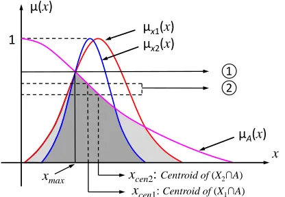
C. Prefiltering module in Cen-NSFLC
Figure 5 shows two different input FSs, i.e.X1 andX2,
which are intersected with an antecedent A. Although the actual input FSs are different, the firing levels calculated by the standard approach are the same in both cases, as shown in circle 1 in the Fig. 5. Thus, two different inputs or more specifically, inputs with a different associated uncertainty distribution result in the same firing level and thus FLC out-put. Hence, a method with a more detailed capture of input certainty and its intersection with the respective antecedent FS is desirable, i.e. the new method should have a higher sensitivity to the shape of the intersection.
1 μ(x)
xmax
μx1(x)
μA(x) μx2(x)
① ②
xcen1: Centroid of (X1∩A) xcen2: Centroid of (X2∩A)
x
Fig. 5: The difference between the Sta-NSFLC and Cen-NSFLC. (Adapted from [14], [15])
Figure 5 shows how in Sta-NSFLCs the maximum of the intersection between the antecedent and different input FSs result in the same xmax and thus the same firing
level. However, the firing strengths in the Cen-NSFLC, i.e.
xcen1 and xcen2, are different when the centroid of each
intersection has been applied instead of their maximum. Given a discrete FS X with a MF xX(xi), the Centroid
is defined as below:
xcen(X) =
Pn
i=1xiµX(xi)
Pn
i=1µX(xi)
, (28)
wheren is the number of discretization levels (n= 100in our case) utilized in a discrete system.
As detailed in [14], [15], the centroid of the intersection of an inputX and an antecedent A, i.e. centroid ofX∩A, the new input/output mapping is defined as:
µY(y) =µX∩A(xcen(X∩A))? µC(y). (29)
Alternatively, for minimum t-norm:
µY(y) = min[µX∩A(xcen(X∩A)), µC(y)]. (30)
[image:4.612.67.286.256.349.2]IV. SIMULATIONSTUDIES
A series of quadcopter UAV simulation experiments are discussed using the SFLC, Sta-NSFLC and Cen-NSFLC introduced in the previous sections. Figure 6 shows the block diagram of the experimental setup where the output from each FLC, i.e., desired velocity (21), is sent as input to the UAV’s velocity controller. A number of tests are made considering different levels of noise and fuzzifier for the FLCs.
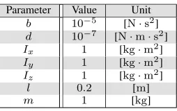
A. Intrinsic parameters of the Quadcopter and its Initial State
[image:5.612.114.241.262.342.2]Table I shows the quadcopter’s intrinsic parameters, which are used in (1) and (19). These parameters are chosen to be close to the ones of a real quadcopter.
TABLE I: The quadcopter’s intrinsic parameters.
Parameter Value Unit
b 10−5 [N·s2] d 10−7 [N·m·s2]
Ix 1 [kg·m2]
Iy 1 [kg·m2]
Iz 1 [kg·m2]
l 0.2 [m]
m 1 [kg]
The quadcopter is first hovering, therefore, the quadcopter initial state of (20) is
x0=
0 0 0 0 0 0 0 0 0 0 0 0 T
.
B. Uncertainty Sources in Measurements
In our paper, the goal is to control the position and yaw angle of the quadcopter(x, y, z, ψ)without considering external disturbances, e.g., wind. Therefore, we need to measure the actual position and yaw angle of the quad-copter(x, y, z, ψ). In order to obtain these measurements we simulate a key set of standard onboard quadcopter sensors with different levels of noise. In our case the noise level is
characterised by its standard deviation σN. Hence, we can
convertσN to SNR, which is also commonly used to describe
the noise, using the following relation:
SNR = 10 log10
1
σ2 N
. (31)
In order to have the measurement of the quadcopter’s position (¯x,y¯ andz¯) we simulate the GPS. To produce the noisy position measurements we add white Gaussian noise to the true position:
¯
x=N(x, σN2) (32)
¯
y=N(y, σ2N) (33)
¯
z=N(z, σ2N), (34)
whereN(µ, σ2)is the Gaussian distribution with meanµand variance σ2. Our simulated GPS computes a new position
every100ms, as the real one.
To measure the yaw angle of the quadcopter ψ¯, we simulate the IMU. The IMU provides us the measurements of orientation (φ¯,θ¯andψ¯) and angular velocities in body frame (¯p,q¯andr¯). In order to produce the noisy measurements for the yaw angle we also add white Gaussian noise to the true yaw angle:
¯
ψ=Nψ, σN2 (1 + 3r)2. (35)
C. Fuzzifiers for NSFLC
As the fuzzifier discussed in Section III, the Gaussian distribution is applied for the inputs of the NSFLCs. Figure 7 shows the different levels of fuzzifier utilized in our exper-iments, representing different levels of expected uncertainty or noise.
D. Membership Function and Rule Base of FLC
In our work, Gaussian distribution is employed for the input and output membership functions (MFs) of FLC. Each input variable, i.e., error or time derivative of the error, has
Quadcopter UAV
GPS Standard
Non-Singleton FLC (Sta-NSFLC)
Centroid Non-Singleton FLC (Cen-NSFLC)
Singleton FLC (SFLC)
Fuzzy Logic Controller (FLC)
Noise
IMU
Switch
Sensors Switch
Velocity Control
V∗
𝑥 , 𝑦
[image:5.612.63.555.537.699.2]𝑧 , 𝜓
x 0
0.5 1
σ F=0.25 σ
F=0.5 σ
F=0.75 σ
F=1 σ
F=1.5 σ
[image:6.612.314.558.50.158.2]F=2
Fig. 7: Different levels of fuzzifier for the NSFLC.
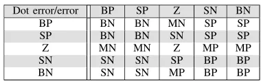
[image:6.612.56.304.51.145.2]five MFs, and the output variable has seven MFs. Table II shows the rule base of FLC, as utilized in [21], where each abbreviation N, Z, P, B, M or S represents negative, zero, positive, big, medium or small, respectively.
TABLE II: Rule Base of FLC
Dot error/error BP SP Z SN BN
BP BN BN MN SP SP
SP BN BN SN SP SP
Z MN MN Z MP MP
SN SN SN SP BP BP
BN SN SN MP BP BP
E. Performance Evaluation
The control performance evaluation is carried out in terms of the mean squared error (MSE) of the 3D position,epos:
epos=
1
n
n
X
k=1
p
(x(k)−x∗)2+ (y(k)−y∗)2+ (z(k)−z∗)2,
(36) where x(k), y(k) and z(k) are the translations along x-,
y- andz-axis, and x∗, y∗ andz∗ represent the desired 3D position. And the mean absolute error (MAE) of yaw angle,
eyaw:
eyaw=
1
n
n
X
k=1
|ψ(k)−ψ∗| (37)
whereψ(k) is the yaw angle andψ∗ represents the desired yaw angle.
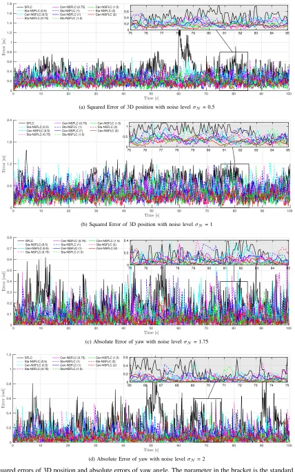
F. Results
To illustrate the performance comparison of the different FLCs, the obtained results are presented in Table III and Table IV. Figure 8 shows four visualised results of the squared errors in 3D position and absolute errors in yaw angle under different input noise levels (σN). In general,
the control performances of NSFLCs are better than the ones of SFLC. When we increase the spread parameter (σF,
as the parameters shown in the brackets in Fig. 8) for the fuzzifier in the NSFLC, the performance of the NSFLC gets better, and the Cen-NSFLC outperforms the Sta-NSFLC, especially with larger input noise levels. Finally, we can observe that all the FLCs provide better performances when noise level decreases. In addition, we can also clearly find the performance differences among the SFLC, Sta-NSFLC and Cen-NSFLC in Fig. 9 below.
Noise LevelσN
0.25 0.5 0.75 1 1.25 1.5 1.75 2
M
S
E
E
r
r
o
r
[m
]
0 0.5 1 1.5
SFLC Sta-NSFLC(σ
F=1)
Cen-NSFLC(σ F=1)
Sta-NSFLC(σ F=2)
Cen-NSFLC(σ F=2)
Fig. 9: Performance comparison of SFLC and NSFLCs.
V. CONCLUSION ANDFUTUREWORK
In this paper, a comprehensive evaluation of quadcotper UAV control performance has been conducted with three different types of FLCs, i.e., a SFLC and two novel NSFLCs (Sta-NSFLC and Cen-NSFLC), under different levels of input noise (uncertainty). The objective of this work was not only to evaluate the performances of the Sta-NSFLC and the SFLC, but also to compare the control performances between the Sta-NSFLC and the Cen-NSFLC. The extensive simu-lated experiments show that the Sta-NSFLC outperforms the SFLC in the most of cases, and the Cen-NSFLC can obtain better control performances compared to the Sta-NSFLC, especially at the higher input noise levels. Additionally, the various levels of fuzzifier show the different capabilities to capture a specified amount of uncertainty, i.e. the higher level fuzzifier has more capability to manage higher level input noise. These results support the results in [14], [15].
For future work, we will focus on conducting experi-ments on real-world quadcopter UAVs while also exploring different Type-2 FLCs for navigating quadcopter UAV, and compare their performances in a variety of input noise levels.
ACKNOWLEDGMENT
The research was partially supported by the ST Engi-neering - NTU Corporate Lab through the NRF corporate lab@university scheme. This work was also partially funded by the RCUK’s EP/M02315X/1 From Human Data to Per-sonal Experience grant.
REFERENCES
[1] N. Michael, S. Shen, K. Mohta, Y. Mulgaonkar, V. Kumar, K. Na-gatani, Y. Okada, S. Kiribayashi, K. Otake, K. Yoshida, K. Ohno, E. Takeuchi, and S. Tadokoro, “Collaborative mapping of an earthquake-damaged building via ground and aerial robots,”Journal of Field Robotics, vol. 29, no. 5, pp. 832–841, 2012.
[2] C. Fu, A. Carrio, M. Olivares-Mendez, R. Suarez-Fernandez, and P. Campoy, “Robust real-time vision-based aircraft tracking from Unmanned Aerial Vehicles,” inRobotics and Automation (ICRA), 2014 IEEE International Conference on, 2014, pp. 5441–5446.
[3] V. Andaluz, E. Lpez, D. Manobanda, F. Guamushig, F. Chicaiza, J. Snchez, D. Rivas, F. Prez, C. Snchez, and V. Morales, “Nonlinear Controller of Quadcopters for Agricultural Monitoring,” inAdvances in Visual Computing, ser. Lecture Notes in Computer Science, 2015, vol. 9474, pp. 476–487.
[image:6.612.79.269.254.313.2]Time [s]
0 10 20 30 40 50 60 70 80 90 100
E
rr
or
[m
]
0 0.2 0.4 0.6 0.8 1 1.2 1.4 1.6 1.8
SFLC Sta-NSFLC (0.5) Cen-NSFLC (0.5) Sta-NSFLC (0.75)
Cen-NSFLC (0.75) Sta-NSFLC (1) Cen-NSFLC (1) Sta-NSFLC (1.5)
Cen-NSFLC (1.5) Sta-NSFLC (2) Cen-NSFLC (2)
75 76 77 78 79 80 81 82 83 84 85
0 0.2 0.4 0.6
(a) Squared Error of 3D position with noise levelσN = 0.5
Time [s]
0 10 20 30 40 50 60 70 80 90 100
E
rr
or
[m
]
0 0.6 1.2 1.8 2.4
SFLC Sta-NSFLC (0.5) Cen-NSFLC (0.5) Sta-NSFLC (0.75)
Cen-NSFLC (0.75) Sta-NSFLC (1) Cen-NSFLC (1) Sta-NSFLC (1.5)
Cen-NSFLC (1.5) Sta-NSFLC (2) Cen-NSFLC (2)
75 76 77 78 79 80 81 82 83 84 85
0 0.5 1
(b) Squared Error of 3D position with noise levelσN = 1
Time [s]
0 10 20 30 40 50 60 70 80 90 100
E
rr
or
[r
ad
]
0 0.1 0.2 0.3 0.4 0.5 0.6 0.7 0.8
SFLC Sta-NSFLC (0.5) Cen-NSFLC (0.5) Sta-NSFLC (0.75)
Cen-NSFLC (0.75) Sta-NSFLC (1) Cen-NSFLC (1) Sta-NSFLC (1.5)
Cen-NSFLC (1.5) Sta-NSFLC (2) Cen-NSFLC (2)
75 76 77 78 79 80 81 82 83 84 85
0 0.2 0.4
(c) Absolute Error of yaw with noise levelσN = 1.75
Time [s]
0 10 20 30 40 50 60 70 80 90 100
E
rr
or
[r
ad
]
0 0.2 0.4 0.6 0.8 1 1.2
SFLC Sta-NSFLC (0.5) Cen-NSFLC (0.5) Sta-NSFLC (0.75)
Cen-NSFLC (0.75) Sta-NSFLC (1) Cen-NSFLC (1) Sta-NSFLC (1.5)
Cen-NSFLC (1.5) Sta-NSFLC (2) Cen-NSFLC (2)
65 66 67 68 69 70 71 72 73 74 75
0 0.2 0.4 0.6
[image:7.612.93.521.49.734.2](d) Absolute Error of yaw with noise levelσN = 2
Fig. 8: Squared errors of 3D position and absolute errors of yaw angle. The parameter in the bracket is the standard deviation
TABLE III: Average MSE of 3D Positiion (Unit: Meter)
FLC / Noise Level (σN) 0 0.25 0.5 0.75 1 1.25 1.5 1.75 2
Singleton FLC 1.4447×10⁻¹⁵ 0.2035 0.3930 0.4813 0.6678 0.7871 0.9152 1.0040 1.0393
[image:8.612.88.521.264.439.2]Sta-NSFLC (σF=0.25) 1.2694×10⁻¹² 0.1501 0.2900 0.4366 0.5830 0.7708 0.9088 1.0823 1.2533 Cen-NSFLC (σF=0.25) 1.8813×10⁻¹² 0.1663 0.3057 0.4272 0.5422 0.7080 0.8303 0.9975 1.1680 Sta-NSFLC (σF=0.5) 1.9668×10⁻¹² 0.1506 0.2555 0.4113 0.5477 0.6580 0.8138 0.9816 1.0387 Cen-NSFLC (σF=0.5) 1.6627×10⁻¹² 0.1125 0.2158 0.3308 0.4059 0.5500 0.6164 0.7262 0.8465 Sta-NSFLC (σF=0.75) 1.1863×10⁻¹² 0.1365 0.2486 0.3840 0.4853 0.6121 0.7504 0.8810 1.0028 Cen-NSFLC (σF=0.75) 1.8213×10⁻¹³ 0.0999 0.1885 0.2627 0.3500 0.4329 0.5442 0.6316 0.7289 Sta-NSFLC (σF=1) 1.6388×10⁻¹² 0.1163 0.2403 0.3609 0.4867 0.6027 0.6915 0.8338 0.9023 Cen-NSFLC (σF=1) 1.7542×10⁻¹² 0.0930 0.1672 0.2472 0.3381 0.3980 0.4648 0.5339 0.5957 Sta-NSFLC (σF=1.25) 1.3936×10⁻¹⁴ 0.1246 0.2356 0.3515 0.4582 0.5721 0.6941 0.8215 0.9192 Cen-NSFLC (σF=1.25) 1.4813×10⁻¹⁴ 0.1024 0.1777 0.2471 0.3133 0.4079 0.4598 0.5695 0.6125 Sta-NSFLC (σF=1.5) 1.4123×10⁻¹⁴ 0.1197 0.2143 0.3410 0.3929 0.5487 0.6837 0.8117 0.8989 Cen-NSFLC (σF=1.5) 2.3086×10⁻¹⁴ 0.0877 0.1503 0.2219 0.2976 0.3907 0.4384 0.5102 0.6427 Sta-NSFLC (σF=1.75) 1.5418×10⁻¹² 0.1080 0.1975 0.3294 0.4249 0.5587 0.6395 0.7674 0.8269 Cen-NSFLC (σF=1.75) 1.2412×10⁻¹² 0.0805 0.1630 0.2133 0.2793 0.3842 0.4314 0.5260 0.6289 Sta-NSFLC (σF=2) 1.7693×10⁻¹⁴ 0.1123 0.2111 0.3071 0.3767 0.5121 0.6545 0.6760 0.7853 Cen-NSFLC (σF=2) 1.7184×10⁻¹⁴ 0.0748 0.1462 0.2100 0.2846 0.3520 0.4063 0.5033 0.5608
TABLE IV: Average MAE of Yaw (Unit: Radian)
FLC / Noise Level (σN) 0 0.25 0.5 0.75 1 1.25 1.5 1.75 2
Singleton FLC 8.3566×10⁻¹⁶ 0.0157 0.0320 0.0491 0.0753 0.1152 0.1344 0.1629 0.2256
Sta-NSFLC (σF=0.25) 7.3227×10⁻¹³ 0.0144 0.0356 0.0515 0.0669 0.0707 0.0972 0.1042 0.1174 Cen-NSFLC (σF=0.25) 1.0855×10⁻¹² 0.0309 0.0377 0.0626 0.0758 0.0871 0.0951 0.1030 0.1155 Sta-NSFLC (σF=0.5) 1.1355×10⁻¹² 0.0237 0.0408 0.0488 0.0716 0.0702 0.0973 0.1090 0.1142 Cen-NSFLC (σF=0.5) 9.5998×10⁻¹³ 0.0136 0.0348 0.0398 0.0500 0.0670 0.0730 0.0782 0.0908 Sta-NSFLC (σF=0.75) 6.8491×10⁻¹³ 0.0177 0.0256 0.0418 0.0512 0.0610 0.0721 0.1019 0.0970 Cen-NSFLC (σF=0.75) 1.0515×10⁻¹³ 0.0142 0.0232 0.0309 0.0360 0.0437 0.0543 0.0583 0.0706 Sta-NSFLC (σF=1) 9.4595×10⁻¹³ 0.0199 0.0285 0.0448 0.0688 0.0651 0.0817 0.0957 0.1031 Cen-NSFLC (σF=1) 1.0128×10⁻¹² 0.0148 0.0205 0.0322 0.0462 0.0501 0.0555 0.0608 0.0826 Sta-NSFLC (σF=1.25) 8.0445×10⁻¹⁵ 0.0188 0.0286 0.0355 0.0509 0.0550 0.0661 0.0819 0.0989 Cen-NSFLC (σF=1.25) 8.5523×10⁻¹⁵ 0.0140 0.0228 0.0271 0.0323 0.0387 0.0432 0.0479 0.0573 Sta-NSFLC (σF=1.5) 8.1205×10⁻¹⁵ 0.0112 0.0222 0.0347 0.0436 0.0532 0.0697 0.0809 0.0743 Cen-NSFLC (σF=1.5) 1.3331×10⁻¹⁴ 0.0092 0.0165 0.0241 0.0306 0.0314 0.0445 0.0490 0.0479 Sta-NSFLC (σF=1.75) 8.9016×10⁻¹³ 0.0107 0.0187 0.0346 0.0474 0.0579 0.0591 0.0767 0.0849 Cen-NSFLC (σF=1.75) 7.1659×10⁻¹³ 0.0081 0.0179 0.0231 0.0352 0.0328 0.0380 0.0501 0.0602 Sta-NSFLC (σF=2) 1.0358×10⁻¹⁴ 0.0121 0.0225 0.0304 0.0409 0.0542 0.0629 0.0740 0.0823 Cen-NSFLC (σF=2) 9.9232×10⁻¹⁵ 0.0094 0.0155 0.0213 0.0320 0.0312 0.0364 0.0442 0.0525
[5] I. Sa and P. Corke, “Vertical Infrastructure Inspection Using a Quad-copter and Shared Autonomy Control,” inField and Service Robotics, ser. Springer Tracts in Advanced Robotics, 2014, vol. 92, pp. 219–232. [6] C. Fu, A. Carrio, and P. Campoy, “Efficient visual odometry and mapping for Unmanned Aerial Vehicle using ARM-based stereo vision pre-processing system,” inUnmanned Aircraft Systems (ICUAS), 2015 International Conference on, 2015, pp. 957–962.
[7] J. Pestana, I. Mellado-Bataller, J. L. Sanchez-Lopez, C. Fu, I. F. Mon-dragon, and P. Campoy, “A General Purpose Configurable Controller for Indoors and Outdoors GPS-Denied Navigation for Multirotor Unmanned Aerial Vehicles,”Journal of Intelligent & Robotic Systems, vol. 73, no. 1-4, pp. 387–400, 2014.
[8] F. Rinaldi, S. Chiesa, and F. Quagliotti, “Linear Quadratic Control for Quadrotors UAVs Dynamics and Formation Flight,” Journal of Intelligent & Robotic Systems, vol. 70, no. 1, pp. 203–220, 2012. [9] J. R. Hervas, M. Reyhanoglu, H. Tang, and E. Kayacan, “Nonlinear
control of fixed-wing UAVs in presence of stochastic winds,” Com-munications in Nonlinear Science and Numerical Simulation, vol. 33, pp. 57–69, 2016.
[10] E. Kayacan, E. Kayacan, H. Ramon, and W. Saeys, “Nonlinear modeling and identification of an autonomous tractortrailer system,” Computers and Electronics in Agriculture, vol. 106, pp. 1–10, 2014. [11] C. Fu, M. A. Olivares-Mendez, R. Suarez-Fernandez, and P. Campoy,
“Monocular Visual-Inertial SLAM-Based Collision Avoidance Strat-egy for Fail-Safe UAV Using Fuzzy Logic Controllers,” Journal of Intelligent & Robotic Systems, vol. 73, no. 1-4, pp. 513–533, 2014. [12] A. Cara, I. Rojas, H. Pomares, C. Wagner, and H. Hagras, “On
comparing non-singleton type-1 and singleton type-2 fuzzy controllers for a nonlinear servo system,” in Advances in Type-2 Fuzzy Logic
Systems (T2FUZZ), 2011 IEEE Symposium on, 2011, pp. 126–133.
[13] G. Mouzouris and J. Mendel, “Dynamic non-singleton fuzzy logic systems for nonlinear modeling,”Fuzzy Systems, IEEE Transactions on, vol. 5, no. 2, pp. 199–208, 1997.
[14] A. Pourabdollah, C. Wagner, and J. Aladi, “Changes under the hood - a new type of non-singleton fuzzy logic system,” inFuzzy Systems (FUZZ-IEEE), 2015 IEEE International Conference on, 2015, pp. 1–8. [15] A. Pourabdollah, C. Wagner, and J. M. Garibaldi, “Improved Uncer-tainty Capture for Non-Singleton Fuzzy Systems,” inFuzzy Systems, IEEE Transactions on, 2016.
[16] S. Bouabdallah, “Design and control of quadrotors with application to autonomous flying,” Ph.D. dissertation, EPFL, 2 2007.
[17] R. Mahony, V. Kumar, and P. Corke, “Multirotor Aerial Vehicles: Mod-eling, Estimation, and Control of Quadrotor,” Robotics Automation Magazine, IEEE, vol. 19, no. 3, pp. 20–32, 2012.
[18] V. Mistler, A. Benallegue, and N. M’Sirdi, “Exact linearization and noninteracting control of a 4 rotors helicopter via dynamic feedback,” inRobot and Human Interactive Communication, 2001. Proceedings. 10th IEEE International Workshop on, 2001, pp. 586–593.
[19] A. Sarabakha, “Reactive obstacle avoidance for quadrotor UAVs based on dynamic feedback linearization,” Master’s thesis, 2015.