To Compress, or Not to Compress:Characterizing Deep Learning Model Compression for Embedded Inference

(1)

To Compress, or Not to Compress:

Characterizing Deep Learning Model

Compression for Embedded Inference

Qing Qin‡, Jie Ren†, Jialong Yu‡, Ling Gao‡, Hai Wang‡, Jie Zheng‡, Yansong Feng§, Jianbin Fang¶, Zheng Wang∗

‡ _{Northwest University, China,}† _{Shaanxi Normal University, China,}§ _{Peking University, China} ¶ _{National University of Defense Technology, China,}∗ _{Lancaster University, United Kingdom}

Abstract—The recent advances in deep neural networks (DNNs) make them attractive for embedded systems. However, it can take a long time for DNNs to make an inference on resource-constrained computing devices. Model compression techniques can address the computation issue of deep inference on embedded devices. This technique is highly attractive, as it does not rely on specialized hardware, or computation-offloading that is often infeasible due to privacy concerns or high latency. However, it remains unclear how model compression techniques perform

across a wide range of DNNs. To design efficient embedded

deep learning solutions, we need to understand their behaviors. This work develops a quantitative approach to characterize model compression techniques on a representative embedded deep learning architecture, the NVIDIA Jetson Tx2. We perform extensive experiments by considering 11 influential neural net-work architectures from the image classification and the natural language processing domains. We experimentally show that how two mainstream compression techniques, data quantization and pruning, perform on these network architectures and the implications of compression techniques to the model storage size, inference time, energy consumption and performance metrics. We demonstrate that there are opportunities to achieve fast deep inference on embedded systems, but one must carefully choose the compression settings. Our results provide insights on when and how to apply model compression techniques and guidelines for designing efficient embedded deep learning systems.

Keywords-Deep learning, embedded systems, parallelism, en-ergy efficiency, deep inference

I. INTRODUCTION

In recent years, deep learning has emerged as a powerful tool for solving complex problems that were considered to be difficult in the past. It has brought a step change in the machine’s ability to perform tasks like object recognition [9], [15], facial recognition [21], [26], speech processing [1], and machine translation [2]. While many of these tasks are also important on mobiles and the Internet of Things (IoT), existing solutions are often computation-intensive and require a large amount of resources for the model to operate. As a result, performing deep inference1 _{on embedded devices can lead}

to long runtime and the consumption of abundant amounts of resources, including CPU, memory, and power, even for simple tasks [3]. Without a solution, the hoped-for advances on embedded sensing will not arrive.

Numerous approaches have been proposed to accelerate deep inference on embedded devices. These include designing purpose-built hardware to reduce the computation or memory latency [10], compressing a pre-trained model to reduce its storage and memory footprint as well as computational re-quirements [13], and offloading some, or all, computation to

1_{Inference in this paper refers to apply a pre-trained model on an input to}

obtain the corresponding output. This is different from statistical inference.

a cloud server [18], [28]. Compared to specialized hardware, model compression techniques have the advantage of being readily deployable on commercial-off-the-self hardware; and compared to computation offloading, compression enables local, on-device inference which in turn reduces the response latency and has fewer privacy concerns. Such advantages make model compressions attractive on resource-constrained embedded devices where computation offloading is infeasible. However, model compression is not a free lunch as it comes at the cost of loss in prediction accuracy [6]. This means that one must carefully choose the model compression technique and its parameters to effectively trade precision for time, energy, as well as computation and resource requirements. Furthermore, as we will show in this paper, the reduction in the model size does not necessarily translate into faster infer-ence time. Because there is no guarantee for a compression technique to be profitable, we need to know when and how to apply a compression technique.

Our work aims to characterize deep learning model com-pression techniques for embedded inference. Knowing this not only assists the better deployment of computation-intensive models, but also informs good design choices for deep learning models and accelerators.

To that end, we develop a quantitative approach to charac-terize two mainstream model compression techniques, prun-ing [6] and data quantization [11]. We apply the techniques to the image classification and the natural language processing (NLP) domains, two areas where deep learning has made great breakthroughs and a rich set of pre-trained models are available. We evaluate the compression results on the NVIDIA Jetson TX2 embedded deep learning platform and consider a wide range of influential deep learning models including convolutional and recurrent neural networks.

We show that while there is significant gain for choosing the right compression technique and parameters, mistakes can seriously hurt the performance. We then quantify how different model compression techniques and parameters af-fect the inference time, energy consumption, model storage requirement and prediction accuracy. As a result, our work provides insights on when and how to apply deep learning model compression techniques on embedded devices, as well as guidelines on designing schemes to adapt deep learning model optimisations for various application constraints.

The main contributions of this workload characterization

paper are two folds:

• We present the first comprehensive study for deep learn-ing model compression techniques on embedded systems; • Our work offers new insights on when and how to apply

(2)

V G G _ 1 6 R e s N e t _ 5 0

0

1 0 0 2 0 0 3 0 0 4 0 0 5 0 0 6 0 0

B e f o r e c o m p r e s s i o n A f t e r p r u n i n g A f t e r q u a n t i z a t i o n

S

to

ra

g

e

s

iz

e

(

M

B

)

(a) Model size

V G G _ 1 6 R e s N e t _ 5 0

0

3 0 6 0 9 0 1 2 0 1 5 0

In

fe

re

n

c

e

t

im

e

(

m

s

)

(b) Inference time

V G G _ 1 6 R e s N e t _ 5 0 0 . 0

0 . 2 0 . 4 0 . 6 0 . 8 1 . 0 1 . 2 1 . 4

E

n

e

rg

y

c

o

n

s

u

m

p

ti

o

n

(J

)

(c) Energy consunption

V G G _ 1 6 R e s N e t _ 5 0

0

1 0 2 0 3 0 4 0 5 0 6 0 7 0 8 0 9 0 1 0 0

A

c

u

ra

c

y

(

%

)

[image:2.612.53.565.64.156.2]

(d) Accuracy

Figure 1: The achieved model size (a) inference time (b) energy consumption (c) and accuracy (d) before and after the compression byquantizationandpruning. The compression technique to use depends on the optimization target.

II. BACKGROUND ANDMOTIVATION

A. Background

In this work, we consider two commonly used model compression techniques, described as follows.

Pruning. This technique removes less important parameters and pathways from a trained network. Pruning ranks the neurons in the network according how much the neuron contribute, it then removes the low ranking neurons to reduce the model size. Care must be taken to not remove too many neurons to significantly damage the accuracy of the network.

Data quantization.This technique reduces the number of bits used to store the weights of a network, e.g., using 8 bits to represent a 32-bit floating point number. In this work, we apply data quantization to convert a pre-trained floating point model into a fixed point model without re-training. We use 6, 8 and 16 bits to represent a 32-bit number, as these are the most common fixed-pointed data quantization configurations [12].

B. Motivation

Choosing the right compression technique is non-trivial. As a motivation example, consider applying pruning and

data quantization, to two representative convolutional neural

networks (CNN),VGG_16and Resnet_50, for image clas-sification. Our evaluation platform is a NVIDIA Jetson TX2 embedded platform (see Section III-A).

Setup. We apply each of the compression techniques to the pre-trained model (which has been trained on the ImageNet ILSVRC 2012 training dataset [17]). We then test the original and the compressed models on ILVRSC 2012 validation set which contains 50k images. We use the GPU for inferencing.

Motivation Results. Figure 1 compares the model size, in-ference time, energy consumption and accuracy after applying compression. By removing some of the nerons of the network,

pruning is able to reduces the inference time and energy

consumption by 28% and 22.5%, respectively. However, it offers little saving in storage size because network weights still dominate the model size. By contrast, by using a few number of bits to represent the weights, quantization significantly reduces the model storage size by 75%. However, the reduction in the model size does not translate to faster inference time and fewer energy consumption; on the contrary, the inference time and energy increase by 1.41x and 1.19x respectively. This is because the sparsity in network weights brought by

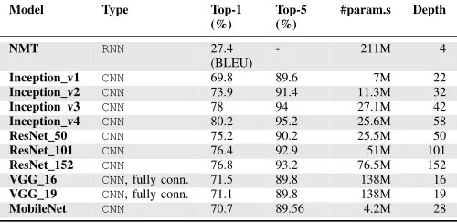
Table I: List of deep learning models considered in this work.

Model Type Top-1

(%)

Top-5 (%)

#param.s Depth

NMT RNN 27.4

(BLEU)

- 211M 4

Inception v1 CNN 69.8 89.6 7M 22

Inception v2 CNN 73.9 91.4 11.3M 32

Inception v3 CNN 78 94 27.1M 42

Inception v4 CNN 80.2 95.2 25.6M 58

ResNet 50 CNN 75.2 90.2 25.5M 50

ResNet 101 CNN 76.4 92.9 51M 101

ResNet 152 CNN 76.8 93.2 76.5M 152

VGG 16 CNN, fully conn. 71.5 89.8 138M 16

VGG 19 CNN, fully conn. 71.1 89.8 138M 19

MobileNet CNN 70.7 89.56 4.2M 28

quantizationleads to irregular computation which causes poor

GPU performance [4] and the cost of de-quantization (details in Section IV-E) . Applying both compression techniques has modest impact on the prediction accuracy, on average, less than 5%. This suggests that both techniques can be profitable.

Lessons Learned. This example shows that the compression technique to use depends on what to be optimized for. If storage space is a limiting factor,quantizationprovides more gains overpruning, but a more powerful processor unit is re-quired to achieve quick on-device inference. If faster on-device turnaround time is a priority,pruning can be employed but it would require sufficient memory resources to store the model parameters. As a result, the profitability of the compression technique depends on the optimization constraints. This work provides an extensive study to characterize the benefits and cost of the two model compression techniques.

III. EXPERIMENTALSETUP

A. Platform and Models

Hardware.Our experimental platform is the NVIDIA Jetson TX2 embedded platform. The system has a 64 bit dual-core Denver2 and a 64 bit quad-core ARM Cortex-A57 running at 2.0 Ghz, and a 256-core NVIDIA Pascal GPU running at 1.3 Ghz. The board has 8 GB of LPDDR4 RAM and 96 GB of storage (32 GB eMMC plus 64 GB SD card).

System Software.We run the Ubuntu 16.04 operating system with Linux kernel v4.4.15. We use Tensorflow v.1.6, cuDNN (v6.0) and CUDA (v8.0.64).

Deep Learning Models. We consider 10 pre-trained CNN

[image:2.612.313.563.201.323.2]

(3)

machine translation. Table I lists the models considered in this work. The chosen models have different parameter sizes and network depths, and thus cover a wide range of CNNand

RNNmodel architectures. We applydata quantization toCNN

models because the current Tensorflow implementation does not support quantization ofRNNs. Aspruningrequires model updates through retraining, we consider three typical models

for pruning to keep the experiment manageable.

B. Evaluation Methodology

Performance Metrics We consider the following metrics:

• Inference time(lower is better). Wall clock time between

a model taking in an input and producing an output, excluding the model load time.

• Power/Energy consumption(lower is better). The energy

used by a model for inference. We deduct the static power used by the hardware when the system is idle.

• Accuracy(higher is better). The ratio of correctly labeled

images to the total number of testing instances.

• Precision (higher is better). The ratio of a correctly

predicted instances to the total number of instances that are predicted to have a specific label. This metric answers e.g., “Of all the images that are labeled to have a cat,

how many actually have a cat?”.

• Recall(higher is better). The ratio of correctly predicted

instances to the total number of test instances that belong to an object class. This metric answers e.g., “Of all the test images that have a cat, how many are actually

labeled to have a cat?”.

• F1 score (higher is better). The weighted average of

Precision and Recall, calculated as2×Recall×P recision Recall+P recision. It is useful when the test dataset has an uneven distribution of classes.

• BLEU(higher is better). The bilingual evaluation

under-study (BLEU) evaluates the quality of machine transla-tion. The quality is considered to be the correspondence between a machine’s output and that of a human: “the closer a machine translation is to a professional human

translation, the better it is”. We report the BLUE value

on NMT, a machine translation model.

Performance Report.For image recognition, the accuracy of a model is evaluated using the top-1 score by default; and we also consider the top-5 score. We use the definitions given by the ImageNet Challenge. Specifically, for the top-1 score, we check if the top output label matches the ground truth label of the primary object; and for the top-5 score, we check if the ground truth label of the primary object is in the top 5 of the output labels for each given model. For NLP, we use the aforementioned BLEU metric. Furthermore, to collect inference time and energy consumption, we run each model on each input repeatedly until the 95% confidence bound per model per input is smaller than 5%. In the experiments, we exclude the loading time of theCNNmodels as they only need to be loaded once in practice. To measure energy consumption, we developed a runtime to take readings from the on-board

power sensors at a frequency of 1,000 samples per second. We matched the power readings against the time stamps of model execution to calculate the energy consumption, while the power consumption is the mean of all the power readings.

IV. EXPERIMENTALRESULTS

A. Roadmap

In this section, we first quantify the computational charac-teristics of deep learning models. Next, we investigate how

quantization and pruning affect the model storage size and

memory footprint. We then look at whether the reduction in the model size can translate into faster inference time and lower power usage and energy consumption, as well as the implications of compression settings to the precision metrics. Finally, we evaluate whether it is beneficial for combining both compress techniques.

B. Model Computational Characteristics

The first task of our experiments is to understand the computational characteristics for the deep learning models considered in this work. Figure 2 quantifies how different type of neural network operations contribute to the inference time across models. The numbers are averaged across the test samples for each model – 50K for image classifiers and 10K for NMT. To aid clarity, we group the operations into seven classes, listed from A to G in the table on the right-hand side. Note that we only list operations that contribute to at least 1% of execution time.

Each cell of the heatmap represents the percentage that a specific type of operation contributes to the model inference time. As can be seen from the figure, a handful of operations are collectively responsible for over 90% of the model execu-tion time. However, the types of operaexecu-tions that dominate the inference time vary across networks. Unsurprisingly, CNNs

are indeed dominated by convolution, while fully-connected networks andRNNsdepend heavily on matrix multiplications.

C. Impact on the Model Storage Size

Reducing the model storage size is crucial for storage-constrained devices. A smaller model size also translates to smaller runtime memory footprint of less RAM space usage. Figures 3, 4 and 5 illustrate how the different compression techniques and parameters affect the resulting model size.

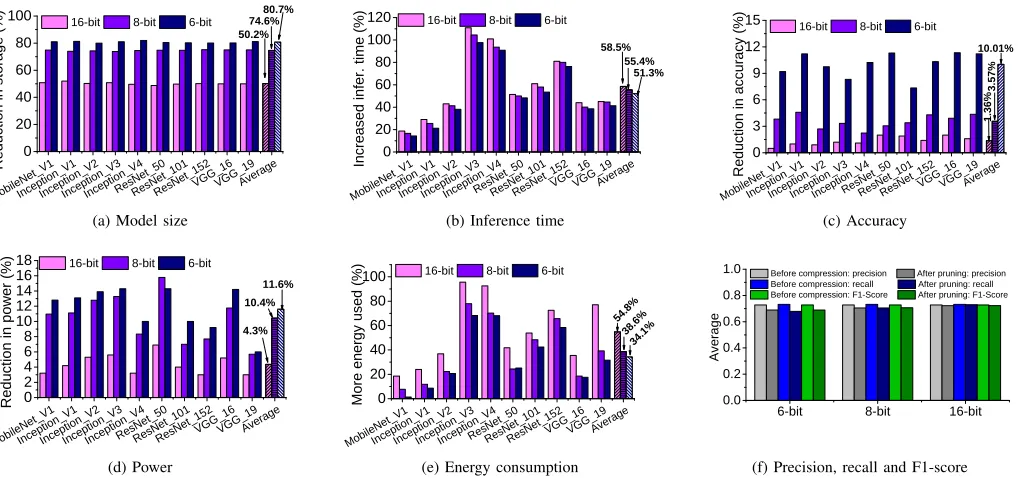
As can be seen from Figure 3a, data quantization can sig-nificantly reduce the model storage size, leading to an average reduction of 50.2% when using a 16-bit representation and up to 80.7% when using a 6-bit representation. The reduction in the storage size is consistent across neural networks as the size of a network is dominated by its weights.

From Figure 4a, we see that by removing some of the neurons of a network,pruningcan also reduce the model size, although the gain is smaller than quantization if we want to keep the accuracy degradation within 5%. On average,pruning

(4)

&RQY'

'&G1DWLYH

$YJ3RRO 0D[SRO 0DW0XO

0XO $GG 6XE _6XP 7LOH

7UDQVSRVH 4'0DQ\9 FRQFDWY9 5HOX _5VTUW ,GHQWLW\ 9DULDEOH9 0RELOHQHWBY ,QFHSWLRQBY ,QFHSWLRQBY ,QFHSWLRQBY ,QFHSWLRQBY 5HV1HWB 5HV1HWB 5HV1HWB 9**B 9**B 107 3HUFHQWDJH

A B C D E F G

Group OP Class

A Convolution

B Matrix

Operations

C Elementwise

Arithmetic

D Reduction and

Expansion

E Data

Movement

F Vector

Operations

[image:4.612.99.519.55.208.2]

G Others

Figure 2: Breakdown of execution time per operation type per deep learning model. Only operations that contribute to a least 1% of the inference time are shown.

M ob i l e Ne t _

V 1

I n ce p t i on _

V 1

I n ce p t i on _

V 2

I n ce p t i on _

V 3

I n ce p t i on _

V 4 R es N

e t _5 0 R es N

e t _1 0

1

R es N e t _1 5

2

V G G _ 1 6 V G G _

1 9 A ve r a

g e 0 2 0 4 0 6 0 8 0

1 0 0 _{7 4 . 6 %}8 0 . 7 %

5 0 . 2 %

R e d u c ti o n i n s to ra g e ( % )

1 6 - b i t 8 - b i t 6 - b i t

(a) Model size

M ob i l e Ne t _

V 1

I n ce p t i on _

V 1

I n ce p t i on _

V 2

I n ce p t i on _

V 3

I n ce p t i on _

V 4 R es N

e t _5 0 R es N

e t _1 0

1

R es N e t _1 5

2

V GG _ 1 6 V G G _

1 9 A ve r a

g e 0 2 0 4 0 6 0 8 0 1 0 0 1 2 0

In c re a s e d i n fe r. t im e ( % )

1 6 - b i t 8 - b i t 6 - b i t

5 1 . 3 % 5 5 . 4 % 5 8 . 5 %

(b) Inference time

M ob i l e Ne t _

V 1

I n ce p t i on _

V 1

I n ce p t i on _

V 2

I n ce p t i on _

V 3

I n ce p t i on _

V 4 R es N

e t _5 0 R es N

e t _1 0

1

R es N e t _1 5

2

V GG _ 1 6 V G G _

1 9 A ve r a

g e 0 3 6 9 1 2 1 5 R e d u c ti o n i n a c c u ra c y ( % )

1 6 - b i t 8 - b i t 6 - b i t

1 0 . 0 1 %

3 .5 7 % 1 .3 6 % (c) Accuracy

M ob i l e N e t _

V 1

I n ce p t i on _

V 1

I n ce p t i on _

V 2

I n ce p t i on _

V 3

I n ce p t i on _

V 4 R es N

e t _5 0 R es N

e t _1 0

1

R es N e t _1 5

2

V G G _ 1 6 V GG _

1 9 A ve r a

g e 0 2 4 6 8 1 0 1 2 1 4 1 6 1 8 R e d u c ti o n i n p o w e r (%

) _{1 6 - b i t} _{8 - b i t} _{6 - b i t}

1 1 . 6 % 1 0 . 4 %

4 . 3 %

(d) Power

M ob i l e Ne t _

V 1

I n ce p t i on _

V 1

I n ce p t i on _

V 2

I n ce p t i on _

V 3

I n ce p t i on _

V 4 R es N

e t _5 0 R es N

e t _1 0

1

R es N e t _1 5

2

V GG _ 1 6 V G G _

1 9 A ve r a

g e 0 2 0 4 0 6 0 8 0 1 0 0

M o re e n e rg y u s e d ( %

) _{1 6 - b i t} _{8 - b i t} _{6 - b i t}

3 4. 1

%

3 8. 6

%

5 4. 8

%

(e) Energy consumption

6 - b i t 8 - b i t 1 6 - b i t 0 . 0

0 . 2 0 . 4 0 . 6 0 . 8 1 . 0

A v e ra g e

B e f o r e c o m p r e s s i o n : p r e c i s i o n A f t e r p r u n i n g : p r e c i s i o n

B e f o r e c o m p r e s s i o n : r e c a l l A f t e r p r u n i n g : r e c a l l

B e f o r e c o m p r e s s i o n : F 1 - S c o r e A f t e r p r u n i n g : F 1 - S c o r e

[image:4.612.56.565.242.481.2]

(f) Precision, recall and F1-score

Figure 3: The achieved model size (a) inference time (b) accuracy (c) power consumption (d) energy consumption (e) and precision, recall and F1-score (e) before and after the compression by quantization.

V G G _ 1 6 R e s n e t 5 0 N M T A v e r a g e

0 2 0 4 0 6 0 8 0 R e d u c ti o n i n s to ra g e ( % )

2 7 . 2 %

(a) Model size

0 1 0 2 0 3 0 4 0 5 0 R e d u c . in i n fe r. t im e ( % )

3 1 %

(b) Inference time

V g g _ 1 6 R e s n e t _ 5 0 A v e r a g e

0 1 2 3 4 5 6 7 8 R e d u c ti o n i n B L E U ( % ) R e d u c ti o n i n a c c u ra c y ( % )

T o p - 1 T o p - 5

5 . 7 %

1 . 7 %

N M T

0 1 2 3 4 5 6 7 8 (c) Accuracy

0 4 8 1 2 1 6 2 0 R e d u c ti o n i n p o w e r (% )

9 . 1 6 %

(d) Power consumption

0

2 0 4 0 6 0

3 6 . 1 %

R e d u c ti o n i n e n e rg y (% )

(e) Energy consumption

P r e c i s i o n R e c a l l F 1 - s c o r e 0 . 0

0 . 2 0 . 4 0 . 6 0 . 8 1 . 0

A v e ra g e

B e f o r e c o m p r e s s i o n A f t e r p r u n i n g

(f) precision, recall and F1 score

[image:4.612.58.564.514.689.2]

(5)

5 % 1 0 % 1 5 % 2 0 % 2 5 %

0

2 0 4 0 6 0 8 0

R

e

d

u

c

ti

o

n

f

o

r

d

if

fe

re

n

t

p

ru

n

in

g

t

h

re

s

h

o

ld

(

%

) T i m e

A c c u r a c y P o w e r E n e r g y

(a) VGG 16

5 % 1 0 % 1 5 % 2 0 % 2 5 %

0

1 0 2 0 3 0 4 0

R

e

d

u

c

ti

o

n

f

o

r

d

if

fe

re

n

t

p

ru

n

in

g

t

h

re

s

h

o

ld

(

%

) _{T i m e}

A c c u r a c y P o w e r E n e r g y

(b) ResNet 50

1 5 % 3 0 % 4 5 % 6 0 % 7 5 %

0

1 0 2 0 3 0 4 0 5 0 6 0

R

e

d

u

c

ti

o

n

f

o

r

d

if

fe

re

n

t

p

ru

n

in

g

t

h

re

s

h

o

ld

(

%

) _{T i m e}

B L E U P o w e r E n e r g y

[image:5.612.57.559.64.163.2]

(c) NMT

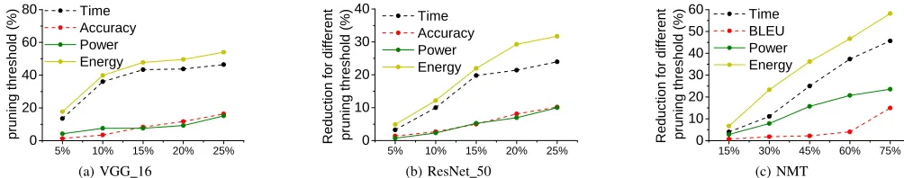
Figure 5: The resulting inference time, accuracy, and power and energy consumption for VGG 16 (a), ResNet 50 (b) andNMT

(c) when using different pruning thresholds. The x-axis shows the percentage of pruning in model size.

M ob i l e Ne t _

V 1

I n ce p t i on _

V 1

I n ce p t i on _

V 2

I n ce p t i on _

V 3

I n ce p t i on _

V 4

R es N e t _5 0 R es N

e t _1 0

1

R es N e t _1 5

2

V GG _ 1 6 V GG _

1 9 A ve r a

g e

0

1 0 2 0 3 0 4 0 5 0

2 2 . 3 % 2 0 . 2 % 9 . 3 % 1 6 - b i t 8 - b i t 6 - b i t

R

e

d

u

c

ti

o

n

i

n

m

e

m

o

ry

f

o

tf

ri

n

t

(%

)

(a)quantization

0

5

1 0 1 5 2 0 2 5 3 0

1 6 . 8 % 1 7 . 9 % B e f o r e c o m p r e s s i o n A f t e r p r u n i n g

M

e

m

o

ry

f

o

tp

ri

n

t

(%

)

(b)pruning

Figure 6: Memory footprint before and after applying

quanti-zation(a) and pruning(b).

observation is that,pruningis particularly effective for obtain-ing a compact model for NMT, an RNN, with a reduction of 60% on the model storage size. This is because there are many repetitive neurons (or cells) in anRNNdue to the natural of the network architecture. As we will discuss later, pruning only causes a minor degradation in the prediction accuracy forNMT. This suggests that pruning can be an effective compression technique forRNNs.

In Figure 5, we compare the resulting performance after using different pruning thresholds from 5% to 75% on two

CNNand aRNNmodels. Increasing the pruning percentage of model size provides more opportunities forpruningto remove more neurons to improve the inference time and other metrics. The improvement reaches a plateau at 15% of reduction for

CNNs, but for NMT, a RNN, the reduction of inference time increases as we remove more neurons. This diagram reinforces our findings that pruning is more effective on RNNs than

CNNs. For the rest discussions of this paper, we use a 5%

pruning threshold.

D. Memory Footprint

Figure 6 compares the runtime memory footprint consumed by a compressed model. Quantization reduces the model memory footprint by 17.2% on average. For example, an 8-bit representation gives a memory footprint saving from 20.02% to 15.97% across networks, with an averaged reduction of 20.2% (up to 40%). In general, the smaller the model is, the less memory footprint it will consume. As an example, a 6-bit representation uses 2.6% and 13.6% less memory compared to an 8-bit and a 16-bit counterparts, respectively.

Figure 6 suggests thatpruningoffers little help in reducing the model memory footprint. On average, it gives a 6.1% reduction of runtime memory footprint. This is because that

the network weights still domain the memory resource con-sumption, and pruning is less effective compared to data

quantizationfor reducing the overhead of network weights.

E. Impact on Inference Time

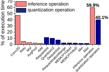
Figure 3b compares the inference time when using different bit widths to represent a 32-bit floating number for neural network weights. Intuitively, a smaller model should run faster. However, data quantization does not shorten the inference time but prolongs it. The reasons are described as follows. Data quantization can speedup the computation (i.e., matrix multiplications) performed on some of the input data by avoiding expensive floating point arithmetics and enabling SIMD vectorization by using a compact data representation. However, we found that the overhead of the de-quantization process during inference can outweigh its benefit. Besides the general inference operation, a data quantization and de-quantization function has to be added into the compressed model. Inference performed on a quantized model accounts for 59.9% of its running time. The de-quantization functions converts input values back to a 32-bit representation on some of the layers (primarily the output layer) in order to recover the loss in precision. As can be seen from Figure 7, this process could be expensive, contributing to 30% to 50% of the inference time.

Using fewer bits for representation can reduce the overhead of de-quantization. For example, using a 6-bit representation is 1.05x and 1.03x faster than using a 16-bit and a 8-bit representations, respectively. However, as we will demonstrate later when discussing Figure 3c, using fewer bits has the drawback of causing larger degradation in the prediction accuracy. Hence, one must carefully find a balance between the storage size, inference time, and prediction accuracy when applying data quantification.

We also find that the percentage of increased inference time depends on the neural network structure. Applying data quantization toInception, the most complex network in our

CNN tested set, will double the inference time. By contrast, data quantization only leads to a 20% increase in inference time for Mobilenet, a compact model. This observation suggests that data quantization may be beneficial for simple neural networks on resource-constrained devices.

In contrast to quantization, Figure 4b shows that pruning

(6)

because there is no extra overhead added to a pruned network. We see that the inference time ofVGG_16andNMTcan benefit from this technique, with an reduction of 38%. Overall, the average inference time is reduced by 31%. This suggests that whilepruningis less effective in reducing the model size (see Section IV-C), it is useful in achieving a faster inference time.

F. Impact on the Power and Energy Consumption

Power and energy consumption are two limiting factors on battery-powered devices. As we can see from Figure 3d,

quantization decreases the peak power usage for inferencing

with an average value of 4.3%, 10.4% and 11.6%, respectively when using a 6-bit, an 8-bit and a 16-bit representations. While

quantization reduces the peak power the device draws, the

increased inference time leads to more energy consumption (which is a product of inference time×instantaneous power) by at least 34.1% and up to 54.8% (see Figure 3e). This means that although quantization allows one to reduces supplied power and voltage, it can lead to a short battery life.

Figure 4e quantifies the reduced energy consumption by applying pruning. Note that it saves over 40%, 15% and 50% energy consumption forVGG_16,ResNet_50andNMT

respectively. Despite that achieving only minor decreases in the peak power usage compared to quantization (9.16% vs 34.1% to 51.1%), the faster inference time ofpruningallows it to reduce the energy consumption. The results indicatepruning

is useful for reducing the overall energy consumption of the system, but quantization can be employed to support a low power system.

G. Impact on The Prediction Accuracy

Accuracy is obviously important for any predictive model because a small and faster model is not useful if it gives wrong predictions all the time.

Results in Figure 3c compare how the prediction accuracy is affected by model compression. We see that the sweat spot of

quantizationdepends on the neural network structure. An

16-bit representation keeps the most information of the original model and thus leads to little reduction in the prediction accuracy, on average 1.36%. Using an 8-bit representation would lead on average 3.57% decrease in the accuracy, while using a 6-bit representation will lead to a significantly larger reduction of 10% in accuracy. We also observe that some networks are more robust toquantization. For example, while a 6-bit representation leads to less than 10% decrease in accuracy for ResNet_101, it cause a 12% drop in accuracy

for ResNet_50. This is because a more complex network

(i.e.,ResNet_101in this case) is more resilient to the weight errors compared to a network (i.e., ResNet_50in this case) with a smaller number of layers and neurons. Our findings suggest the need for having an adaptive scheme to choose the optimaldata quantizationparameter for given constraints.

For pruning, Figure 4c compares the reduction in the

top-1 and the top-5 scores for VGG_16 and ResNet_50. We also show the BLEU value forNMT. Overall,pruningreduces the accuracy of the twoCNN models with by 5.7% and 1.7%

Co n v 2D Re l

u

Mu l Av g Po o

l

Ad d

Re q u an t

i ze

Qu a n ti z

e V2

De q u an t

i ze

Re q u an t

i za t i on R

a ng e

ME MC

PYD t oH

ME MC

PYH t oD Mi n Ma x

i nf e r en c

e o p e ra t

i on

q ua n t i za t

i on o pe r

a ti o n

0

1 0 2 0 3 0 4 0 5 0 6 0 7 0

i n f e r e n c e o p e r a t i o n q u a n t i z a t i o n o p e r a t i o n

4 0 . 1 % 5 9 . 9 %

%

o

f

e

x

e

c

u

ti

o

n

t

im

[image:6.612.351.528.57.174.2]

e

Figure 7: Breakdown of the averaged execution time per operation type, averaging across the quantized models.

respectively for the top-1 and the top-5 scores. It has little negative impact on NMTwhere we only observe an averaged loss of 2.1% for BLEU. When taking into consideration that

pruning can significantly reduce the model size for NMT

(Section IV-C), our results suggest thatpruningis particularly effective forRNNs.

H. Precision, Recall and F1-Score

Figures 3f and 4f show other three performance metrics of a

classificationmodel after applying quantizationandpruning.

We can see that, the decrease in performance after compression is less than 3% for precision, recall and the F1-score. For

quantization, the 16-bit representation outperforms the other

two bits width representations. Specifically, a 16-bit represen-tation gives the highest overall precision, which in turns leads to the best F1-score. High precision can reduce false positive, which is important for certain domains like video surveillance because it can reduce the human involvement for inspecting false positive predictions.

I. Impact of Model Parameter Sizes

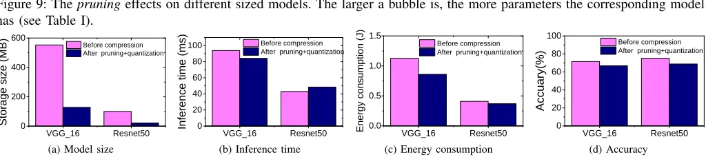
The bubble charts in Figures 8 and 9 quantify the impact by applyingquantizationandpruningto the deep learning models of different sizes. Here, each bubble corresponds to a model. The size of the bubble is proportional to the number of network parameters (see Table I). As can be seen from the diagrams, there is a non-trivial correlation between the original model size, compression techniques, and the optimization constraints. This diagram suggests that there is a need for adaptive schemes like parameter search to effectively explore the design space of multiple optimization objectives.

J. Combining Pruning and Quantization

So far we have evaluated pruning and quantization in isolation. An natural question to ask is: “Is it worthwhile to combine both techniques?”. Figure 10 shows the results by first applying a 8-bit data quantization and then pruning to

VGG_16andResNet50.

(7)

2 2.5 3 3.5 4 4.5 5

0 50 100 150 200 250 300

Los

s i

n

accur

acy

(%)

Inference time (ms)

MobileNet Inception_V1 Inception_V2 ResNet_50 ResNet_101 Inception_V3 VGG_16 VGG_19 ResNet_152 Inception_V4

(a) Inference time vs accuracy

2 2.5 3 3.5 4 4.5 5

0 0.5 1 1.5 2 2.5 3

Loss

in

acc

ur

acy

(%)

Energy (J)

MobileNet Inception_V1 Inception_V2 ResNet_50 ResNet_101 Inception_V3 VGG_16 ResNet_152 VGG_19 Inception_V4

(b) Energy vs accuracy

2 2.5 3 3.5 4 4.5 5

0 50 100 150

Loss

in

acc

ur

acy

(%)

Storage size (ms)

MobileNet Inception_V1 Inception_V2 ResNet_101 Inception_V3 ResNet_50 VGG_16 ResNet_152 VGG_19 Inception_V4

[image:7.612.53.561.61.167.2]

(c) Compressed model size vs accuracy

Figure 8: The quantization effects on different sized models. The larger a bubble is, the more parameters the corresponding model has (see Table I).

0 2 4 6 8

0 50 100 150 200 250

Loss

in acc

ur

ac

y

(%)

Inference time (ms)

VGG_16 ResNet_50 NMT

(a) Inference time vs accuracy

0 2 4 6 8

0 0.5 1 1.5 2 2.5 3

Los

s i

n accu

racy

(%)

Energy (J)

(b) Energy vs accuracy

0 2 4 6 8

0 100 200 300 400 500 600

Los

s in

accu

racy

(%)

Model size (MB)

[image:7.612.58.562.195.299.2]

(c) Compressed model size vs accuracy

Figure 9: Thepruningeffects on different sized models. The larger a bubble is, the more parameters the corresponding model has (see Table I).

V G G _ 1 6 R e s n e t 5 0

0

2 0 0 4 0 0 6 0 0

B e f o r e c o m p r e s s i o n A f t e r p r u n i n g + q u a n t i z a t i o n

S

to

ra

g

e

s

iz

e

(

M

B

)

(a) Model size

V G G _ 1 6 R e s n e t 5 0

0

2 0 4 0 6 0 8 0

1 0 0 B e f o r e c o m p r e s s i o n A f t e r p r u n i n g + q u a n t i z a t i o n

In

fe

re

n

c

e

t

im

e

(

m

s

)

(b) Inference time

V G G _ 1 6 R e s n e t 5 0 0 . 0

0 . 5 1 . 0 1 . 5

E

n

e

rg

y

c

o

n

s

u

m

p

ti

o

n

(

J

)

(c) Energy consumption

V G G _ 1 6 R e s n e t 5 0

0

2 0 4 0 6 0 8 0 1 0 0

A

c

u

a

ry

(%

)

(d) Accuracy

Figure 10: The model size (a) inference time (b) energy consumption (c) and accuracy (d) before and after model compression.

the combination has positive impact on the inference time for

VGG_16 as the runtime overhead of data quantization (see

Section IV-E) can be amortized bypruning. The combination, however, leads to longer inference time forResNet50due to the expensive de-quantization overhead as we have explained. Because of the difference in inference time, there is less benefit in energy consumpation forResNet50overVGG_16

(Figure 10c). This experiment shows that combining pruning

andquantizationcan be beneficial, but it depends on the neural

network architecture and what to optimize for.

V. DISCUSSIONS

Our evaluation reveals thatdata quantizationis particularly effective in reducing the model storage size and runtime memory footprint. As such, it is attractive for devices with limited memory resources, particularly for small-formed IoT devices. However,quantizationleads to longer inference time due to the overhead of the de-quantization process. Therefore, future research is needed to look at reducing the overhead of de-quantization. We also observe that an 8-bit integer quantization seems to be a good trade-off between the model storage size and the precision. This strategy also enables SIMD vectorization on CPUs and GPUs as multiple 8-bit

scalar values can be packed into one vector register. Using less than 8 bits is less beneficial on traditional CPUs and GPUs, but could be useful on FGPAs or specialized hardware with purpose-built registers and memory load/store units. We believe studying when and how to applydata quantizationto a specific domain or a neural network architecture would be an interesting research direction.

We empirically show that pruning allows us to precisely control in the prediction precision. This is useful for applica-tions like security and surveillance where we need a degree of confidences on the predictive outcome. Compared to data

quantization,pruning is less effective in reducing the model

storage size, and thus may require larger storage and memory space. We also find that pruning is particularly effective for

RNNs, perhaps due to the recurrent structures of an RNN. This finding suggests pruning can be an important method for acceleratingRNNon embedded systems.

[image:7.612.52.564.309.423.2]

(8)

to better quantize a model?”. For examples, instead of using just integers, one can use a mixture of floating point numbers and integers with different bit widths by giving wider widths for more important weights. Furthermore, given that it is non-trivial to choose the right compression settings, it will be very useful to have a tool to automatically search over the Pareto design space to find a good configuration to meet the conflict requirements of the model size, inference time and prediction accuracy. As a final remark of our discussion, we hope our work can encourage a new line of research on auto-tuning of deep learning model compression.

VI. RELATEDWORK

There has been a significant amount of work on reducing the storage and computation work by model compression. These techniques include pruning [20], quantization [11], [14], knowledge distillation [16], [22], huffman coding [14], low rank and sparse decomposition [8], decomposition [19], etc. This paper develops a quantitative approach to understand the cost and benefits of deep learning compression techniques. We target pruning and data quantization because these are widely used and directly applicable to a pre-trained model.

In addition to model compression, other works exploit computation-offloading [28], [18], specialized hardware de-sign [5], [13], and dynamic model selection [27]. Our work aims to understand how to accelerate deep learning inference by choosing the right model compression technique. Thus, these approaches are orthogonal to our work.

Off-loading computation to the cloud can accelerate DNN

model inference [28]. Neurosurgeon [18] identifies when it is beneficial (e.g. in terms of energy consumption and end-to-end latency) to offload aDNNlayer to be computed on the cloud. The PervasiveCNN[25] generates multiple computation kernels for each layer of a CNN, which are then dynamically selected according to the inputs and user constraints. A similar approach presented in [23] trains a model twice, once on shared data and again on personal data, in an attempt to prevent personal data being sent outside the personal domain. Com-putation off-loading is not always applicable due to privacy, latency or connectivity issues. Our work is complementary to previous work on computation off-loading by offering insights to best optimize localinference.

VII. CONCLUSIONS

This paper has presented a comprehensive study to char-acterize the effectiveness of model compression techniques on embedded systems. We consider two mainstream model compression techniques and apply them to a wide range of representative deep neural network architectures. We show that there is no “one-size-fits-all” universal compression setting, and the right decision depends on the target neural network architecture and the optimization constraints. We reveal the cause of the performance disparity and demonstrate that a carefully chosen parameter setting can lead to efficient em-bedded deep inference. We provide new insights and concrete

guidelines, and define possible avenues of research to enable efficient embedded inference.

ACKNOWLEDGMENTS

This work was supported in part by the NSF China under grant agreements 61872294 and 61602501; the Fundamental Research Funds for the Central Universities under grant ment GK201803063; the UK EPSRC through grant agree-ments EP/M01567X/1 (SANDeRs) and EP/M015793/1 (DIV-IDEND); and the Royal Society International Collaboration Grant (IE161012). For any correspondence, please contact Jie Ren ([email protected]), Jianbin Fang ([email protected]) and Zheng Wang ([email protected]).

REFERENCES

[1] Dario Amodei et al. Deep speech 2: End-to-end speech recognition in

english and mandarin. InICML ’16.

[2] Dzmitry Bahdanau et al. Neural machine translation by jointly learning

to align and translate.arXiv, 2014.

[3] Alfredo Canziani et al. An analysis of deep neural network models for

practical applications. CoRR, 2016.

[4] Xuhao Chen. Escort: Efficient sparse convolutional neural networks on

gpus.CoRR, 2018.

[5] Yu-Hsin Chen et al. Eyeriss: An energy-efficient reconfigurable

acceler-ator for deep convolutional neural networks.IEEE Journal of Solid-State

Circuits, 2017.

[6] Yu Cheng et al. A survey of model compression and acceleration for

deep neural networks.arXiv, 2017.

[7] Emily L Denton et al. Exploiting linear structure within convolutional

networks for efficient evaluation. InNIPS ’14.

[8] Jeff Donahue et al. Decaf: A deep convolutional activation feature for

generic visual recognition. InICML ’14.

[9] Petko Georgiev et al. Low-resource multi-task audio sensing for mobile and embedded devices via shared deep neural network representations. ACM IMWUT, 2017.

[10] Yunchao Gong et al. Compressing deep convolutional networks using

vector quantization. Computer Science, 2014.

[11] Young H. Oh et al. A portable, automatic data quantizer for deep neural

networks. InPACT, 2018.

[12] Song Han et al. Eie: Efficient inference engine on compressed deep

neural network. InISCA ’16.

[13] Song Han et al. Deep compression: Compressing deep neural networks

with pruning, trained quantization and huffman coding. arXiv, 2015.

[14] Kaiming He et al. Deep residual learning for image recognition. In CVPR ’16.

[15] Geoffrey Hinton et al. Distilling the knowledge in a neural network. arXiv, 2015.

[16] ImageNet. Large Scale Visual Recognition Challenge 2012. http://www. image-net.org/challenges/LSVRC/2012/, 2012.

[17] Yiping Kang et al. Neurosurgeon: Collaborative intelligence between

the cloud and mobile edge. InASPLOS ’17.

[18] Vadim Lebedev et al. Speeding-up convolutional neural networks using

fine-tuned cp-decomposition. arXiv, 2014.

[19] Hao Li et al. Pruning filters for efficient convnets. InICLR ’17.

[20] Omkar M Parkhi et al. Deep face recognition. InBMVC ’15.

[21] Bharat Bhusan Sau and Vineeth N. Balasubramanian. Deep model

compression: Distilling knowledge from noisy teachers. arxiv, 2016.

[22] Sandra Servia-Rodriguez et al. Personal model training under privacy

constraints. InACM IoTDI ’18.

[23] Nathan Silberman and Sergio Guadarrama.

Tensorflow-slim image classification library.

https://github.com/tensorflow/models/tree/master/research/slim, 2013. [24] Mingcong Song et al. Towards pervasive and user satisfactory cnn across

gpu microarchitectures. InHPCA ’17.

[25] Yi Sun, Yuheng Chen, et al. Deep learning face representation by joint

identification-verification. InNIPS ’14.

[26] Ben Taylor et al. Adaptive deep learning model selection on embedded

systems. InLCTES ’18.

[27] Surat Teerapittayanon et al. Distributed deep neural networks over the