Active Learning by Labeling Features
Gregory DruckDept. of Computer Science University of Massachusetts
Amherst, MA 01003
Burr Settles
Dept. of Biostatistics & Medical Informatics Dept. of Computer Sciences
University of Wisconsin Madison, WI 53706
Andrew McCallum
Dept. of Computer Science University of Massachusetts
Amherst, MA 01003
Abstract
Methods that learn from prior informa-tion about input features such as
general-ized expectation (GE) have been used to
train accurate models with very little ef-fort. In this paper, we propose an
ac-tive learning approach in which the
ma-chine solicits “labels” on features rather than instances. In both simulated and real user experiments on two sequence label-ing tasks we show that our active learnlabel-ing method outperforms passive learning with features as well as traditional active learn-ing with instances. Preliminary experi-ments suggest that novel interfaces which intelligently solicit labels on multiple fea-tures facilitate more efficient annotation. 1 Introduction
The application of machine learning to new prob-lems is slowed by the need for labeled training data. When output variables are structured, an-notation can be particularly difficult and time-consuming. For example, when training a condi-tional random field (Lafferty et al., 2001) to ex-tract fields such asrent,contact,features, andutilities
from apartment classifieds, labeling 22 instances (2,540 tokens) provides only 66.1% accuracy.1
Recent work has used unlabeled data and lim-ited prior information about input features to boot-strap accurate structured output models. For ex-ample, both Haghighi and Klein (2006) and Mann and McCallum (2008) have demonstrated results better than 66.1% on the apartments task de-scribed above using only a list of 33 highly dis-criminative features and the labels they indicate. However, these methods have only been applied in scenarios in which the user supplies such prior knowledge before learning begins.
1Averaged over 10 randomly selected sets of 22 instances.
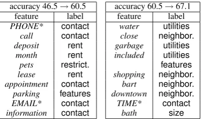
In traditionalactive learning(Settles, 2009), the machine queries the user for only the labels of in-stances that would be most helpful to the machine. This paper proposes an active learning approach in which the user provides “labels” for input features, rather than instances. A labeled input feature de-notes that a particular input feature, for example the word call, is highly indicative of a particular label, such ascontact. Table 1 provides an excerpt of a feature active learning session.
In this paper, we advocate using generalized expectation (GE) criteria (Mann and McCallum, 2008) for learning with labeled features. We pro-vide an alternate treatment of the GE objective function used by Mann and McCallum (2008) and a novel speedup to the gradient computation. We then provide a pool-based feature active learning algorithm that includes an option to skip queries, for cases in which a feature has no clear label. We propose and evaluate feature query selection algorithms that aim to reduce model uncertainty, and compare to several baselines. We evaluate our method using both real and simulated user ex-periments on two sequence labeling tasks. Com-pared to previous approaches (Raghavan and Al-lan, 2007), our method can be used for both classi-fication and structured tasks, and the feature query selection methods we propose perform better.
We use experiments with simulated labelers on real data to extensively compare feature query se-lection algorithms and evaluate on multiple ran-dom splits. To make these simulations more re-alistic, the effort required to perform different la-beling actions is estimated from additional exper-iments with real users. The results show that ac-tive learning with features outperforms both pas-sive learning with features and traditional active learning with instances.
In the user experiments, each annotator actively labels instances, actively labels features one at a time, and actively labels batches of features
accuracy 46.5→60.5 feature label PHONE* contact
call contact
deposit rent
month rent
pets restrict.
lease rent
appointment contact
parking features
EMAIL* contact
information contact
accuracy 60.5→67.1 feature label
water utilities
close neighbor.
garbage utilities
included utilities features
shopping neighbor.
bart neighbor.
downtown neighbor.
TIME* contact
[image:2.595.73.281.61.184.2]bath size
Table 1: Two iterations of feature active learning. Each table shows the features labeled, and the re-sulting change in accuracy. Note that the word in-cludedwas labeled as bothutilitiesandfeatures, and
that∗denotes a regular expression feature.
nized using a “grid” interface. The results support the findings of the simulated experiments and pro-vide epro-vidence that the “grid” interface can facili-tate more efficient annotation.
2 Conditional Random Fields
In this section we describe the underlying proba-bilistic model for all methods in this paper. We focus on sequence labeling, though the described methods could be applied to other structured out-put or classification tasks. We model the proba-bility of the label sequence y ∈ Yn conditioned
on the input sequence x ∈ Xn, p(y|x;θ) using
first-order linear-chain conditional random fields (CRFs) (Lafferty et al., 2001). This probability is
p(y|x;θ) = Z1 xexp
X
i X
j
θjfj(yi, yi+1,x, i),
where Zx is the partition function and feature functions fj consider the entire input sequence
and at most two consecutive output variables. The most probable output sequence and transition marginal distributions can be computed using vari-ants of Viterbi and forward-backward.
Provided a training data distribution p˜, we es-timate CRF parameters by maximizing the condi-tional log likelihood of the training data.
L(θ) =Ep˜(x,y)[logp(y|x;θ)]
We use numerical optimization to maximizeL(θ), which requires the gradient ofL(θ) with respect to the parameters. It can be shown that the par-tial derivative with respect to parameterjis equal
to the difference between the empirical expecta-tion ofFjand the model expectation ofFj, where Fj(y,x) =Pifj(yi, yi+1,x, i).
∂
∂θjL(θ) =Ep˜(x,y)[Fj(y,x)]
−Ep˜(x)[Ep(y|x;θ)[Fj(y,x)]].
We also include a zero-mean variance σ2 = 10 Gaussian prior on parameters in all experiments.2
2.1 Learning with missing labels
The training set may contain partially labeled se-quences. Let z denote missing labels. We esti-mate parameters with this data by maximizing the marginal log-likelihood of the observed labels.
LMML(θ) =Ep˜(x,y)[log
X
z
p(y,z|x;θ)]
We refer to this training method as maximum
marginal likelihood (MML); it has also been
ex-plored by Quattoni et al. (2007).
The gradient of LMML(θ) can also be written
as the difference of two expectations. The first is an expectation over the empirical distribution ofx andy, and the model distribution ofz. The second is a double expectation over the empirical distribu-tion ofxand the model distribution ofyandz.
∂
∂θjLMML(θ) =Ep˜(x,y)[Ep(z|y,x;θ)[Fj(y,z,x)]]
−Ep˜(x)[Ep(y,z|x;θ)[Fj(y,z,x)]].
We train models using LMML(θ) with expected
gradient (Salakhutdinov et al., 2003).
To additionally leverage unlabeled data, we compare with entropy regularization (ER). ER adds a term to the objective function that en-courages confident predictions on unlabeled data. Training of linear-chain CRFs with ER is de-scribed by Jiao et al. (2006).
3 Generalized Expectation Criteria In this section, we give a brief overview of
gen-eralized expectation criteria(GE) (Mann and
Mc-Callum, 2008; Druck et al., 2008) and explain how we can use GE to learn CRF parameters with esti-mates of feature expectations and unlabeled data.
GE criteria are terms in a parameter estimation objective function that express preferences on the
value of a model expectation of some function. Given a score functionS, an empirical distribution ˜
p(x), a model distribution p(y|x;θ), and a con-straint functionGk(x,y), the value of a GE
crite-rion isG(θ) =S(Ep˜(x)[Ep(y|x;θ)[Gk(x,y)]]).
GE provides a flexible framework for parameter estimation because each of these elements can take an arbitrary form. The most important difference between GE and other parameter estimation meth-ods is that it does not require a one-to-one cor-respondence between constraint functionsGkand
model feature functions. We leverage this flexi-bility to estimate parameters of feature-rich CRFs with a very small set of expectation constraints.
Constraint functions Gk can be normalized so
that the sum of the expectations of a set of func-tions is 1. In this case, S may measure the di-vergence between the expectation of the constraint function and a target expectationGˆk.
G(θ) = ˆGklog(E[Gk(x,y)]), (1)
whereE[Gk(x,y)] =Ep˜(x)[Ep(y|x;θ)[Gk(x,y)]].
It can be shown that the partial derivative of G(θ)with respect to parameterjis proportional to the predicted covariance between the model fea-ture functionFjand the constraint functionGk.3
∂
∂θjG(θ) =
ˆ
Gk
E[Gk(x,y)]× (2)
Ep˜(x)Ep(y|x;θ)[Fj(x,y)Gk(x,y)]
−Ep(y|x;θ)[Fj(x,y)]Ep(y|x;θ)[Gk(x,y)]
The partial derivative shows that GE learns pa-rameter values for model feature functions based on their predicted covariance with the constraint functions. GE can thus be interpreted as a boot-strapping method that uses the limited training sig-nal to learn about parameters for related model feature functions.
3.1 Learning with feature-label distributions
Mann and McCallum (2008) apply GE to a linear-chain, first-order CRF. In this section we provide an alternate treatment that arrives at the same ob-jective function from the general form described in the previous section.
Often, feature functions in a first-order linear-chain CRF f are binary, and are the conjunction
3If we use squared error forS, the partial derivative is the
covariance multiplied by2( ˆGk−E[Gk(x,y)]).
of an observational testq(x, i)and a label pair test 1{yi=y0,yi+1=y00}.4
f(yi, yi+1,x, i) =1{yi=y0,yi+1=y00}q(x, i)
The constraint functionsGk we use here
decom-pose and operate similarly, except that they only include a test for a single label. Single label con-straints are easier for users to estimate and make GE training more efficient. Label transition struc-ture can be learned automatically from single la-bel constraints through the covariance-based pa-rameter update of Equation 2. For convenience, we can write Gyk to denote the constraint
func-tion that combines observafunc-tion test k with a test for labely. We also add a normalization constant
Ck=Ep˜(x)[Piqk(x, i)],
Gyk(x,y) = X
i
1
Ck1{yi=y}qk(x, i)
Under this construction the expectation ofGyk is
the predicted conditional probability that the label at some arbitrary positioniisywhen the observa-tional test atisucceeds,p˜(yi=y|qk(x, i)=1;θ).
If we have a set of constraint functions{Gyk : y ∈ Y}, and we use the score function in Equa-tion 1, then the GE objective funcEqua-tion specifies the minimization of the KL divergence between the model and target distributions over labels condi-tioned on the success of the observational test. In general the objective function will consist of many such KL divergence penalties.
Computing the first term of the covariance in Equation 2 requires a marginal distribution over three labels, two of which will be consecutive, but the other of which could appear anywhere in the sequence. We can compute this marginal using the algorithm of Mann and McCallum (2008). As previously described, this algorithm isO(n|Y|3) for a sequence of length n. However, we make the following novel observation: we do not need to compute the extra lattices for feature label pairs withGˆyk = 0, since this makes Equation 2 equal
to zero. In Mann and McCallum (2008), probabil-ities were smoothed so that∀y Gˆyk > 0. If we
assume that only a small number of labelsmhave non-zero probability, then the time complexity of the gradient computation is O(nm|Y|2). In this paper typically1 ≤m≤ 4, while|Y| is 11 or 13.
4We this notation for an indicator function that returns 1
In experiments in this paper, using this optimiza-tion does not significantly affect final accuracy.
We use numerical optimization to estimate model parameters. In general GE objective func-tions are not convex. Consequently, we initial-ize 0th-order CRF parameters using a sliding win-dow logistic regression model trained with GE. We also include a Gaussian prior on parameters withσ2 = 10in the objective function.
3.2 Learning with labeled features
The training procedure described above requires a set of observational tests or input features with target distributions over labels. Estimating a dis-tribution could be a difficult task for an annotator. Consequently, we abstract away from specifying a distribution by allowing the user to assign labels to features (c.f. Haghighi and Klein (2006) , Druck et al. (2008)). For example, we say that the word featurecallhas labelcontact. A label for a feature
simply indicates that the feature is a good indicator of the label. Note that features can have multiple labels, as doesincludedin the active learning ses-sion shown in Table 1. We convert an input feature with a set of labelsLinto a distribution by assign-ing probability1/|L|for eachl∈Land probabil-ity0for eachl /∈L. By assigning 0 probability to labelsl /∈L, we can use the speed-up described in the previous section.
3.3 Related Work
Other proposed learning methods use labeled fea-tures to label unlabeled data. The resulting partially-labeled corpus can be used to train a CRF by maximizing MML. Similarly,prototype-driven
learning (PDL) (Haghighi and Klein, 2006)
opti-mizes the joint marginal likelihood of data labeled
withprototype input features for each label.
Ad-ditional features that indicate similarity to the pro-totypes help the model to generalize. In a previ-ous comparison between GE and PDL (Mann and McCallum, 2008), GE outperformed PDL without the extra similarity features, whose construction may be problem-specific. GE also performed bet-ter when supplied accurate label distributions.
Additionally, both MML and PDL do not natu-rally generalize to learning with features that have multiple labels or distributions over labels, as in these scenarios labeling the unlabeled data is not straightforward. In this paper, we attempt to ad-dress this problem using a simple heuristic: when there are multiple choices for a token’s label,
sam-ple a label. In Section 5 we use this heuristic with MML, but in general obtain poor results.
Raghavan and Allan (2007) also propose sev-eral methods for learning with labeled features, but in a previous comparison GE gave better re-sults (Druck et al., 2008). Additionally, the gen-eralization of these methods to structured output spaces is not straightforward. Chang et al. (2007) present an algorithm for learning with constraints, but this method requires users to set weights by hand. We plan to explore the use of the recently developed related methods of Bellare et al. (2009), Grac¸a et al. (2008), and Liang et al. (2009) in fu-ture work. Druck et al. (2008) provide a survey of other related methods for learning with labeled input features.
4 Active Learning by Labeling Features Feature active learning, presented in Algorithm 1,
is a pool-based active learning algorithm (Lewis
and Gale, 1994) (with a pool of features rather than instances). The novel components of the algorithm are an option to skip a query and the notion that skipping and labeling have different costs. The option to skip is important when us-ing feature queries because a user may not know how to label some features. In each iteration the model is retrained using thetrainprocedure, which
takes as input a set of labeled features C and un-labeled data distribution p˜. For the reasons de-scribed in Section 3.3, we advocate using GE for thetrainprocedure. Then, while the iteration cost cis less than the maximum costcmax, the feature
query q that maximizes the query selection met-ric φis selected. The acceptfunction determines
whether the labeler will labelq. Ifq is labeled, it is added to the set of labeled featuresC, and the label costclabel is added toc. Otherwise, the skip
costcskipis added toc. This process continues for N iterations.
4.1 Feature query selection methods
In this section we propose feature query selection methodsφ. Queries with a higher scores are con-sidered better candidates. Note again that by fea-tures we mean observational tests qk(x, i). It is
Algorithm 1Feature Active Learning
Input: empirical distributionp˜, initial feature constraints C, label costclabel, skip costcskip, max cost per iteration cmax, max iterationsN
Output:model parametersθ
fori= 1toNdo
θ= train(˜p,C)
c= 0
whilec < cmaxdo
q= argmaxqkφ(qk)
ifaccept(q)then
C=C ∪ label(q)
c=c+clabel
else
c=c+cskip
end if end while end for
θ= train(˜p,C)
We propose to select queries that provide the largest reduction in model uncertainty. We notate possible responses to a query qk as gˆ. The Ex-pected Information Gain (EIG)of a query is the expectation of the reduction in model uncertainty over all possible responses. Mathematically, IG is
φEIG(qk) =Ep(ˆg|qk;θ)[Ep˜(x)[H(p(y|x;θ)− H(p(y|x;θˆg)]],
whereθˆg are the new model parameters if the
re-sponse to qk is gˆ. Unfortunately, this method is
computationally intractable. Re-estimatingθgˆwill typically involve retraining the model, and do-ing this for each possible query-response pair is prohibitively expensive for structured output mod-els. Computing the expectation over possible re-sponses is also difficult, as in this paper users may provide a set of labels for a query, and more gen-erallygˆcould be a distribution over labels.
Instead, we propose a tractable strategy for re-ducing model uncertainty, motivated by traditional uncertainty sampling (Lewis and Gale, 1994). We assume that when a user responds to a query, the reduction in uncertainty will be equal to the To-tal Uncertainty (TU), the sum of the marginal en-tropies at the positions where the feature occurs.
φT U(qk) = X
i X
j
qk(xi, j)H(p(yj|xi;θ))
Total uncertainty, however, is highly biased to-wards selecting frequent features. A mean un-certainty variant, normalized by the feature’s count, would tend to choose very infrequent fea-tures. Consequently we propose a tradeoff
be-tween the two extremes, calledweighted uncer-tainty (WU), that scales the mean uncertainty by the log count of the feature in the corpus.
φW U(qk) = log(Ck)φT UC(qk)
k .
Finally, we also suggest an uncertainty-based met-ric calleddiverse uncertainty (DU)that encour-ages diversity among queries by multiplying TU by the mean dissimilarity between the feature and previously labeled features. For sequence labeling tasks, we can measure the relatedness of features using distributional similarity.5
φDU(qk) =φT U(qk)|C|1 X
j∈C
1−sim(qk, qj)
We contrast the notion of uncertainty described above with another type of uncertainty: the en-tropy of the predicted label distribution for the fea-ture, orexpectation uncertainty (EU). As above we also multiply by the log feature count.
φEU(qk) = log(Ck)H(˜p(yi =y|qk(x, i)=1;θ))
EU is flawed because it will have a large value for non-discriminative features.
The methods described above require the model to be retrained between iterations. To verify that this is necessary, we compare against query selec-tion methods that only consider the previously la-beled features. First, we consider a feature query selection method calledcoverage (cov)that aims to select features that are dissimilar from existing labeled features, increasing the labeled features’ “coverage” of the feature space. In order to com-pensate for choosing very infrequent features, we multiply by the log count of the feature.
φcov(qk) = log(Ck)|C|1 X
j∈C
1−sim(qk, qj)
Motivated by the feature query selection method of Tandem Learning (Raghavan and Allan, 2007) (see Section 4.2 for further discussion), we con-sider a feature selection metric similarity (sim)
that is the maximum similarity to a labeled fea-ture, weighted by the log count of the feature.
φsim(qk) = log(Ck) maxj∈C sim(qk, qj)
5sim(q
k, qj)returns the cosine similarity between context
Features similar to those already labeled are likely to be discriminative, and therefore likely to be la-beled (rather than skipped). However, insufficient diversity may also result in an inaccurate model, suggesting thatcoverage should select more use-ful queries thansimilarity.
Finally, we compare with several passive base-lines. Random (rand)assigns scores to features randomly.Frequency (freq)scores input features using their frequency in the training data.
φfreq(qk) = X
i X
j
qk(xi, j)
Top LDA (LDA) selects the top words from 50 topics learned from the unlabeled data using la-tent Dirichlet allocation (LDA) (Blei et al., 2003). More specifically, the wordswgenerated by each topictare ranked using the conditional probability
p(w|t). The word feature is assigned its maximum rank across all topics.
φLDA(qk) = maxt rankLDA(qk, t)
This method will select useful features if the top-ics discovered are relevant to the task. A similar heuristic was used by Druck et al. (2008).
4.2 Related Work
Tandem Learning (Raghavan and Allan, 2007) is an algorithm that combines feature and instance active learning for classification. The algorithm it-eratively queries the user first for instance labels, then for feature labels. Feature queries are selected according to their co-occurrence with important model features and previously labeled features. As noted in Section 3.3, GE is preferable to the meth-ods Tandem Learning uses to learn with labeled features. We address the mixing of feature and in-stance queries in Section 4.3.
In order to better understand differences in fea-ture query selection methodology, we proposed a feature query selection method motivated6 by the method used in Tandem Learning in Section 4.1. However, this method performs poorly in the ex-periments in Section 5.
Liang et al. (2009) simultaneously developed a method for learning with and actively selecting
6The query selection method of Raghavan and Allan
(2007) requires a stack that is modified between queries within each iteration. Here query scores are only updated after each iteration of labeling.
measurements, or target expectations with
associ-ated noise. The measurement selection method proposed by Liang et al. (2009) is based on Bayesian experimental design and is similar to the expected information gain method described above. Consequently this method is likely to be intractable for real applications. Note that Liang et al. (2009) only use this method in synthetic ex-periments, and instead use a method similar to to-tal uncertainty for experiments in part-of-speech tagging. Unlike the experiments presented in this paper, Liang et al. (2009) conduct only simulated active learning experiments and do not consider skipping queries.
Sindhwani (Sindhwani et al., 2009) simultane-ously developed an active learning method that queries for both instance and feature labels that are then used in a graph-based learning algorithm. They find that querying certain features outper-forms querying uncertain features, but this is likely because their query selection method is similar to the expectation uncertainty method described above, and consequently non-discriminative fea-tures may be queried often (see also the discus-sion in Section 4.1). It is also not clear how this graph-based training method would generalize to structured output spaces.
4.3 Expectation Constraint Active Learning
5 Simulated User Experiments
In this section we experiment with an automated oracle labeler. When presented an instance query, the oracle simply provides the true labels. When presented a feature query, the oracle first decides whether to skip the query. We have found that users are more likely to label features that are rel-evant for only a few labels. Therefore, the oracle labels a feature if the entropy of its per occurrence label expectation, H(˜p(yi=y|qk(x, i) = 1;θ)) ≤
0.7. The oracle then labels the feature using a heuristic: label the feature with the label whose expectation is highest, as well as any label whose expectation is at least half as large.
We estimate the effort of different labeling ac-tions with preliminary experiments in which we observe users labeling data for ten minutes. Users took an average of 4 seconds to label a feature, 2 seconds to skip a feature, and 0.7 seconds to la-bel a token. We setup experiments such that each iteration simulates one minute of labeling by set-ting cmax = 60, cskip = 2 andclabel = 4. For
instance active learning, we use Algorithm 1 but without the skip option, and setclabel = 0.7. We
use N = 10 iterations, so the entire experiment simulates 10 minutes of annotation time. For ef-ficiency, we consider the 500 most frequent unla-beled features in each iteration. To start, ten ran-domly selected seed labeled features are provided. We userandom (rand)selection, uncertainty sampling (US)(using sequence entropy, normal-ized by sequence length) and information den-sity (ID) (Settles and Craven, 2008) to select in-stance queries. We use Entropy Regularization (ER) (Jiao et al., 2006) to leverage unlabeled in-stances.7 We weight the ER term by choosing the best8 weight in {10−3,10−2,10−1,1,10} multi-plied by ##unlabeledlabeled for each data set and query se-lection method. Seed instances are provided such that the simulated labeling time is equivalent to la-beling 10 features.
We evaluate on two sequence labeling tasks.
The apartments task involves segmenting 300
apartment classified ads into 11 fields including
features, rent, neighborhood, and contact. We use the same feature processing as Haghighi and Klein (2006), with the addition of context features in a window of±3. Thecora referencestask is to ex-tract 13 BibTeX fields such asauthorandbooktitle
7Results using self-training instead of ER are similar. 8As measured by test accuracy, giving ER an advantage.
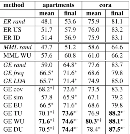
method apartments cora
mean final mean final
ER rand 48.1 53.6 75.9 81.1
ER US 51.7 57.9 76.0 83.2 ER ID 51.4 56.9 75.9 83.1
MML rand 47.7 51.2 58.6 64.6
MML WU 57.6 60.8 61.0 66.2
GE rand 59.0 64.8∗ 77.6 83.7
GE freq 66.5∗ 71.6∗ 68.6 79.8
GE LDA 65.7∗ 71.4∗ 74.9 85.0
GE cov 68.2∗† 72.6∗ 73.5 83.3
GE sim 57.8 65.9∗ 67.1 79.2
GE EU 66.5∗ 71.6∗ 68.6 79.8
GE TU 70.1∗† 73.6∗† 76.9 88.2∗†
GE WU 71.6∗† 74.6∗† 80.3∗† 88.1∗†
[image:7.595.308.527.61.287.2]GE DU 70.5∗† 74.4∗† 78.4∗ 87.5∗†
Table 2: Mean and final token accuracy results. A ∗ or † denotes that a GE method significantly
outperforms all non-GE or passive GE methods, respectively. Bold entries significantly outperform all others. Methods initalicsare passive.
from 500 research paper references. We use a stan-dard set of word, regular expressions, and lexicon features, as well as context features in a window of±3. All results are averaged over ten random 80:20 splits of the data.
5.1 Results
Table 2 presents mean (across all iterations) and final token accuracy results. On the apartments
task, GE methods greatly outperform MML9 and ER methods. Each uncertainty-based GE method also outperforms all passive GE methods. On the
coratask, only GE withweighted uncertainty sig-nificantly outperforms ER and passive GE meth-ods in terms ofmeanaccuracy, but all uncertainty-based GE methods provide higher final accuracy. This suggests that on the cora task, active GE methods are performing better in later iterations. Figure 1, which compares the learning curves of the best performing methods of each type, shows this phenomenon. Further analysis reveals that the uncertainty-based methods are choosing frequent features that are more likely to be skipped than those selected randomly in early iterations.
We next compare with the results of related methods published elsewhere. We cannot make claims about statistical significance, but the results
illustrate the competitiveness of our method. The 74.6% final accuracy onapartmentsis higher than any result obtained by Haghighi and Klein (2006) (the highest is 74.1%), higher than thesupervised
HMM results reported by Grenager et al. (2005) (74.4%), and matches the results of Mann and Mc-Callum (2008) with GE with more accurate sam-pled label distributions and 10 labeled examples. Chang et al. (2007) only obtain better results than 88.2% oncorawhen using 300 labeled examples (two hours of estimated annotation time), 5000 ad-ditional unlabeled examples, and extra test time in-ference constraints. Note that obtaining these re-sults required only 10 simulated minutes of anno-tation time, and that GE methods are provided no information about the label transition matrix.
6 User Experiments
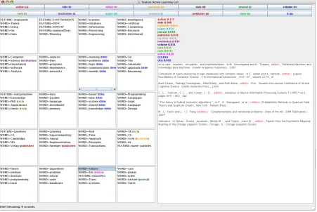
Another advantage of feature queries is that fea-ture names are concise enough to be browsed, rather than considered individually. This allows the design of improved interfaces that can further increase the speed of feature active learning. We built a prototype interface that allows the user to quickly browse many candidate features. The fea-tures are split into groups of five feafea-tures each. Each group contains features that are related, as measured by distributional similarity. The features within each group are sorted according to the ac-tive learning metric. This interface, displayed in Figure 3, may be useful because features in the same group are likely to have the same label.
We conduct three types of experiments. First, a user labels instances selected byinformation den-sity, and models are trained using ER. The in-stance labeling interface allows the user to label tokens quickly by extending the current selection one token at a time and only requiring a single keystroke to label an entire segment. Second, the user labels features presented one-at-a-time by
weighted uncertainty, and models are trained
us-ing GE. To aid the user in understandus-ing the func-tion of the feature quickly, we provide several ex-amples of the feature occurring in context and the model’s current predicted label distribution for the feature. Finally, the user labels features organized using the grid interface described in the previous paragraph. Weighted uncertainty is used to sort feature queries within each group, and GE is used to train models. Each iteration of labeling lasts two minutes, and there are five iterations.
Retrain-ing with ER between iterations takes an average of 5 minutes on cora and 3 minutes on
apart-ments. With GE, the retraining times are on
av-erage 6 minutes oncoraand 4 minutes on
apart-ments. Consequently, even when viewed with
to-tal time, rather thanannotation time, feature active learning is beneficial. While waiting for models to retrain, users can perform other tasks.
Figure 2 displays the results. User 1 labeled
apartmentsdata, while Users 2 and 3 labeledcora
data. User 1 was able to obtain much better results with feature labeling than with instance labeling, but performed slightly worse with the grid inter-face than with the serial interinter-face. User 1 com-mented that they found the label definitions for
apartments to be imprecise, so the other
experi-ments were conducted on the cora data. User 2 obtained better results with feature labeling than instance labeling, and obtained higher mean ac-curacy with the grid interface. User 3 was much better at labeling features than instances, and per-formed especially well using the grid interface.
7 Conclusion
We proposed an active learning approach in which features, rather than instances, are labeled. We presented an algorithm for active learning with features and several feature query selection meth-ods that approximate the expected reduction in model uncertainty of a feature query. In simu-lated experiments, active learning with features outperformed passive learning with features, and uncertainty-based feature query selection outper-formed other baseline methods. In both simulated and real user experiments, active learning with features outperformed passive and active learning with instances. Finally, we proposed a new label-ing interface that leverages the conciseness of fea-ture queries. User experiments suggested that this grid interface can improve labeling efficiency. Acknowledgments
2 4 6 8 10 35
40 45 50 55 60 65 70 75 80
simulated annotation time (minutes)
token accuracy
apartments
ER + uncertainty MML + weighted uncertainty GE + frequency GE + weighted uncertainty
2 4 6 8 10
45 50 55 60 65 70 75 80 85 90
simulated annotation time (minutes)
token accuracy
cora
ER + uncertainty MML + weighted uncertainty GE + random
[image:9.595.124.472.65.202.2]GE + weighted uncertainty
Figure 1: Token accuracy vs. time for best performing ER, MML, passive GE, and active GE methods.
2 4 6 8 10
5 10 15 20 25 30 35 40 45 50 55 60 65
annotation time (minutes)
token accuracy
user 1 − apartments
ER + information density GE + weighted uncertainty (serial) GE + weighted uncertainty (grid)
2 4 6 8 10
30 35 40 45 50 55 60 65 70
annotation time (minutes)
token accuracy
user 2 − cora
ER + information density GE + weighted uncertainty (serial) GE + weighted uncertainty (grid)
2 4 6 8 10
35 40 45 50 55 60 65 70 75 80 85
annotation time (minutes)
token accuracy
user 3 − cora
[image:9.595.72.527.240.366.2]ER + information density GE + weighted uncertainty (serial) GE + weighted uncertainty (grid)
Figure 2: User experiments with instance labeling and feature labeling with theserialandgridinterfaces.
[image:9.595.74.526.407.709.2]References
Kedar Bellare, Gregory Druck, and Andrew McCal-lum. 2009. Alternating projections for learning with expectation constraints. InUAI.
David M. Blei, Andrew Y. Ng, Michael I. Jordan, and John Lafferty. 2003. Latent dirichlet allocation.
Journal of Machine Learning Research, 3:2003.
Ming-Wei Chang, Lev Ratinov, and Dan Roth. 2007. Guiding semi-supervision with constraint-driven learning. InACL, pages 280–287.
Gregory Druck, Gideon Mann, and Andrew McCal-lum. 2008. Learning from labeled features using generalized expectation criteria. InSIGIR.
Joao Grac¸a, Kuzman Ganchev, and Ben Taskar. 2008. Expectation maximization and posterior constraints. In J.C. Platt, D. Koller, Y. Singer, and S. Roweis, editors,Advances in Neural Information Processing Systems 20. MIT Press.
Trond Grenager, Dan Klein, and Christopher D. Man-ning. 2005. Unsupervised learning of field segmen-tation models for information extraction. InACL.
Aria Haghighi and Dan Klein. 2006. Prototype-driven learning for sequence models. InHTL-NAACL.
Feng Jiao, Shaojun Wang, Chi-Hoon Lee, Russell Greiner, and Dale Schuurmans. 2006. Semi-supervised conditional random fields for improved sequence segmentation and labeling. InACL, pages 209–216.
John Lafferty, Andrew McCallum, and Fernando Pereira. 2001. Conditional random fields: Prob-abilistic models for segmenting and labeling se-quence data. InICML.
David D. Lewis and William A. Gale. 1994. A sequen-tial algorithm for training text classifiers. InSIGIR, pages 3–12, New York, NY, USA. Springer-Verlag New York, Inc.
Percy Liang, Michael I. Jordan, and Dan Klein. 2009. Learning from measurements in exponential fami-lies. InICML.
Gideon Mann and Andrew McCallum. 2008. General-ized expectation criteria for semi-supervised learn-ing of conditional random fields. InACL.
A. Quattoni, S. Wang, L.-P Morency, M. Collins, and T. Darrell. 2007. Hidden conditional random fields.
IEEE Transactions on Pattern Analysis and Machine Intelligence, 29:1848–1852, October.
Hema Raghavan and James Allan. 2007. An interac-tive algorithm for asking and incorporating feature feedback into support vector machines. In SIGIR, pages 79–86.
Ruslan Salakhutdinov, Sam Roweis, and Zoubin Ghahramani. 2003. Optimization with em and expectation-conjugate-gradient. In ICML, pages 672–679.
Burr Settles and Mark Craven. 2008. An analysis of active learning strategies for sequence labeling tasks. InEMNLP.
Burr Settles. 2009. Active learning literature survey. Technical Report 1648, University of Wisconsin -Madison.
Vikas Sindhwani, Prem Melville, and Richard D. Lawrence. 2009. Uncertainty sampling and trans-ductive experimental design for active dual supervi-sion. InICML.