Comparative Study of 1 Dimensional Heat Transfer Problem by Finite Difference Method and Finite Element Method

Comparative Study of 1-Dimensional Heat

Transfer Problem by Finite Difference Method and

Finite Element Method

Mr. Vasimakram Khatib1, Mr. Faizan Shaikh2, Mr. Ravindra Hawaldar3, Mr. Madivalappa H4, Mr. Shashank Divgi5

1, 2, 3, 4

UG Mechanical Engineering Student, Girijabai Sail Institute of Technology, Karwar, Karnataka, India

5

Assistant Professor Mechanical Engineering Dept, Girijabai Sail Institute of Technology, Karwar, Karnataka, India

Abstract: Heat transfer is one of the most important sector in Mechanical Engineering. It plays a very important role in sectors like Automobile, Industries and Thermal power plants where the efficiency is depend on the heat flow. As we know the Heat transfer problems can be solved using various methods when the area of the material is known but, it is quite difficult to find the Heat transfer through a body having irregular shapes or where area is not known. This requires many mathematical applications such as Fourier series, Taylor series expansion, Matrix inversion method, Cramer’s method and etc. After this the same problem is solved by Ansys workbench version11 Software which uses Finite Difference method for solving. Once the solution is obtained we draw the graph to show that the results obtained from both methods are equal.

Keywords: Finite Difference method, Finite Element method, Fourier series, Taylor series expansion, Cramer’s method.

I. INTRODUCTION

In this paper we are solving the 1-Dimensional steady state heat transfer problem. By both Finite Difference method as well as Finite Element method. The Finite Difference method includes numerical solutions for this we have to use 1-Dimensionsl steady state heat conduction equation which can be derived by reducing the 3-Dimensional general heat conduction equation in Cartesian co-ordinates that is given by.

+ + + = x (1)

Where T= T(x, y, z)

x, y, z are spatial co-ordinates

α = thermal diffusivity (m2/s), =

ρ= Density (kg/m3)

k= thermal conductivity (W/mK) Cp= Specific heat capacity (J/kgK) g= Internal heat generation.

In this case since we have taken it as a steady state heat transfer problem ( i.e. Temperature does not vary with respect to the time). The governing equation for Finite difference method of solving 1-D heat transfer problem can be derived either with the help of Energy Balance method or even by Taylor series approximation method, both of them will give the same equation.

We have used the Finite difference method because it is one of the most simplest form of solving the given problem numerically, although it involves large number of arithmetic operations to be performed in order to get the results, it also provides a very good insight to the complete problem through which we can analyze the given problem completely.

In case of Finite Element method instead of numerical solutions we have gone for the Ansys workbench software, which gives us the more accurate results and also saves the lot of time since it solves the heat transfer problems very quickly once the input are given. In order to get solutions by Finite element method or -Ansys workbench software we have to made an assumption i.e., since the area of the material is not known we have to assume it as a unit area (1 m2). Once the solutions are obtained from both Finite difference method and Ansys workbench software, we then plot the graph of Temperature v/s Nodes to compare the results.

Generally Finite element method’s can be classified into two types those are, Structural problems and Non- structural problems. The heat transfer problem which we have choose comes under the non- structural problem. Generally there are three phases of finite element method those are, Pre-processing, Solution and Post-processing. Each of these phases have very important role in solving the given problem

Although both Finite difference method and Finite element method are numerical methods of solving the problem they have some differences between them some of those are given below.

1) Finite element method make sure of continuity at nodes and at the boundaries of the element where as Finite difference method will give the continuity at nodal points only.

2) The complicated problems which can be handled by the Finite difference method are very few but Finite element method can handle almost all kind of complicated problems

3) In order to get more good and accurate results Finite difference method need more number of nodes compared to that of the Finite element method.

The 1- Dimensional steady state heat transfer problem which we are solving in this paper is made of a Copper (Cu) material, which has 1 meter length, the initial end that is at x=0 is maintained at the temperature of 1000C and at the end that is at x= 1mis maintained at the temperature of 10000C and the properties of the Cu are,

Thermal conductivity k= 400 W/mK Density ρ= 8960 kg/m3

Specific heat capacity Cp= 386 J/kgK

II. MATERIAL AND METHODOLOGY The methods through which the Heat transfer problems can be solved are

A. Finite Difference method

Finite Difference method is one of the numerical method of solving different types of Engineering problems which are quite difficult to solve by any other methods, by using this method we can solve the Heat transfer problems in the problems where area is not known. It involves some basic steps to be followed and those are given below.

1) Step I: Discretisation; In this step the material is break into smallest possible parts which further cannot be divided.

2) Step II: Naming the nodes is one of the most important step in both finite difference method as well as the finite element method, this involve a basic formula which is given below.

∆x= (2)

Where, L= Length of the material M= Number of nodes and Hence ∆x gives the node of each length.

The figure of the nodal distribution in one dimensional bar of length L having M nodes is shown below.

Fig 1 The above figure shows the nodal distribution in a 1-dimensional element

Step iii: Once the node naming is done the next step is to equate these nodes in the equation, this equation can be generated by the both Energy balance method as well as the Taylor series expansion.

While solving this 1- Dimensional heat conduction problem we have to made some assumptions those are,

The thermal conductivity does not vary along x, y and z directions i.e., kx= ky= kz= k, hence the material is isotropic and homogenous.

The temperature does not vary with respect to the time i.e., steady state. The heat generated g= 0

Hence for One – Dimensional steady state heat conduction with no internal heat generation the equation (1), that is general heat conduction equation in 3D Cartesian co-ordinate becomes

The above is a partial differential equation and can be reduced to a ordinary differential equation that is,

= 0 (4)

Now we integrate the equation (4) with respect to the x Therefore,

= 0 (5)

Now once again integrating the equation (4) with respect to x

T= C1x + C2 (6) C1= integration constant

C2= integration constant

These integration constants are obtained by integrating the equation (4) twice.

In order to solve this we need two boundary conditions and in the given problem we have two boundary conditions that is, At distance x= 0 (at starting point) temperature T= 1000 C

At distance x= 1m (at the end) temperature T= 10000 C Now substituting the values of T in the equation (6), 100= C1(0) + C2

C2= 100.

Similarly now substituting the value of B in boundary condition 2 1000= C1(1) + C2

1000= C1 + 100 C1 = 900.

Therefore the equation (6) becomes

T(x) = 900x + 100 (7)

Now to get the original equation of the finite difference analysis we need to understand the Taylor series expansion. Here we have to use both forward Taylor series expansion as well as the backward Taylor series expansion. By adding both of them we can get the centered difference approximation of the second derivative term, and that is given below.

f(x + ∆x) + f(x - ∆x) = 2f(x) + f”(x)* ∆x2

This can be rearranged as the

f”(x) = [ ( ∆ ) – ( ) ( _{∆ ∗∆} ∆ )] We have the governing equation that is equation no (4)

That is T”(x) = 0; T = T(x); T(x=0)= Tend 1; T(x=L) = Tend 2 Consider this as a equation number (8)

Now we replace this with the second order derivative using the finite difference analysis, we get (Tm-1 – 2Tm + Tm+1) / ∆x2 = 0

Now send the ∆x2 to the right hand side therefore we get,

(Tm-1 – 2Tm + Tm+1) = 0 (8) Where m= location of node.

The equation (8) is the original equation which we are solving. By using this equation we can formulate the nodal equation for finding the temperatures at the nodes where the data is unknown. Once the equation is formulated it can be convert into a matrix of form AT=X. This matrix can be solved by various methods like Gauss elimination method, Gauss-Seidel iterations, Thomas algorithm, Successive over relaxation method and Cramer’s method of solving the matrix, etc.

B. Finite Element Method

In this paper we have selected the Ansys workbench software because we know it follows the procedure of Finite element method to solve the heat transfer problem and also saves the lot of time. Some of the basic and important steps given as input to software are given below.

1) Step i: setting the preferences for the thermal problem

2) Step ii: pre-processor, where element type and type of heat transfer is given as the input.

4) Step iv: giving the material properties such as thermal conductivity of each material that is being used.

5) Step v: giving the node number and location of each node.

6) Step vi: defining the element attribute

7) Step vii: solution

8) Step viii: defining the known values of temperature that is given.

9) Step ix: pos-processing that is obtaining the results once the solution got over. The following is the method of solving the given problem by Finite difference formulation

Fig 2 1-Dimensional figure of given copper bar

The properties of this are Thermal conductivity k= 400 W/mK, Density ρ= 8960 kg/m3, Specific heat capacity Cp= 386 J/kgK In order to solve this we first need to discretise the given domain, here we have divided the given geometry into 5 equal parts which gives us the 6 nodes. The figure of discretised domain is given below

Fig 3 Discretised part of the given 1-D domain.

We already know the temperatures at 1st and 6th nodes

In order to solve this problem we need to consider the interior nodes and apply the equation (8). Now consider node 2, i.e., m=2 for this equation (8) becomes

T1 -2T2 +T3 = 0 Similarly for m=3, 4, 5 equation (8) becomes,

T2 -2T3 +T4 = 0 T3 -2T4 +T5 = 0 T4 -2T5 +T6 = 0

Since T1 and T6 are known values we shift them to the right hand side and equations are rearranged as below -2T2 + T3 = -T1

T2 – 2T3 + T4 = 0 T3 – 2T4 + T5 = 0 T4 - 2T5 = -T6

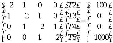
Now we arrange the above equations in the matrix form as shown below.

































2

1

0

0

1

2

1

0

0

1

2

1

0

0

1

2

























5

4

3

2

T

T

T

T





























1000

0

0

100

The above matrix form can be solved by various methods such as Gauss-Siedel elimination, Matrix inversion method, Thomas algorithm, Cramer’s method and etc.

But in this for simple understanding we choose Cramer’s rule. In Cramer’s of solving the given 4x4 matrix we the given matrix is solved with the help of determinants. Once the matrix is solved in order to find the unknown values each column of the 4x4 matrix is replaced by the 1x4 matrix available at the RHS. Therefore now to get the values of the above unknowns we first solve the 4x4 matrix.

D=

2

1

0

0

1

2

1

0

0

1

2

1

0

0

1

2









2

1

0

1

2

1

0

1

2







2

1

0

1

2

0

0

1

1





Now to get the value of D first we need to solve the 3x3 determinant then multiply with the outside values. i.e., =[(-2)x(4-1)] -1x(-2 -0) +0

= - 4 Similarly, the second 3x3 determinant value is

= 1x (4-1) -1x (0) + 0 = 3

Now multiply these values with the outer values, therefore,

D= [(-2)x(-4)] –1x (3) D= 5

Since we have got the value of D, now replacing the each column at a time. Therefore,

D1=

2

1

0

1000

1

2

1

0

0

1

2

0

0

0

1

100











Now to get the unknown values T2, T3, T4and T5 we divide the values of D1, D2, D3 and D4 with D That is

T2= = = 2800 C

Similarly,

T3= = = 4600 C

T4= = = 6400 C

T5= = = 8200 C

Now we have got all the unknown temperatures at the interior nodes 2, 3, 4 and 5 as shown above.

These results obtained are compared with the results obtained by the Ansys software and check whether the values are equal or not.

III. RESULTS AND DISCUSSION

The results are obtained by the Finite difference method, and the temperatures at the each node is listed in the table below and also the graph is plotted.

TABLE I

List of results obtained by Finite difference method Node Temperature

1 100 2 280 3 460 4 640 5 820 6 1000

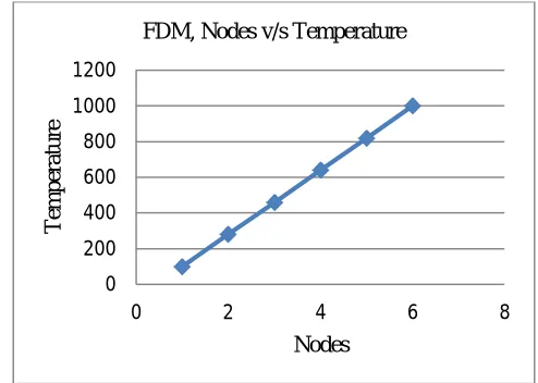
The graph of Nodes v/s Temperature for the above values is plotted below.

Fig 4 Graph of temperature v/s nodes, x-axis; node, y-axis; temperature.

This graph shows the results obtained by the finite difference method. The x-axis represents the nodes and the y-axis represents the temperature. The temperature constantly goes on increasing because temperature at initial end/boundary is maintained at 1000 C and the other end is maintained at 10000 C, this cause the temperature to increase from node to node.

The results obtained from the Finite difference method are also equal to that of the results of Finite difference method and those results with the images of Ansys software are shown below.

0 200 400 600 800 1000 1200

0 2 4 6 8

T

em

pe

ra

ture

Fig 5 Nodal temperature obtained in Ansys software version 11.

TABLE II

List of results obtained by the Ansys software Node Temperature

1 100 2 280 3 460 4 640 5 820 6 1000

The graph of Nodes v/s Temperature for the values obtained by the Ansys software /Finite element method is plotted below.

Fig 6 Graph of Nodes v/s Temperature foe FEM/ Ansys.

The above graph shows the values of temperature at each node obtained by the Ansys software. The x-axis shows the nodes and y-axis shows the values of temperature. By observing this graph we easily say that the results obtained by both the methods are equal.

IV. CONCLUSION

By the results obtained above we can easily tell that both Finite Difference method as well as the Finite Element method (Ansys) gives the equal values. The time consumed by the Ansys software is very less as compared to that of the Finite Difference Analysis but still we have assumed the area as the unity (1 m2) to get the solution in Finite Element method without which it was not quite possible to solve this problem, where in Finite difference method we don’t need the area to solve the problem, all we need is that the given body has to be divide into a equal portions or nodes. This gives the advantage for FDM by which we can solve the heat transfer problems of a body having unknown areas and irregular shapes. Using this we can also calculate the heat transfer rate from any of the materials which are being used in automobiles as well as the industries and we can also avoid the possible failure of the material. And can analyze the behavior of the materials subjected to the high temperatures.

0 500 1000 1500

0 2 4 6 8

T

em

pe

ra

ture

REFERENCES

[1] Manuraj Sahu, Gulab Chand Sahu, Manoj Sao and Abhishek Kumar Jain, Analysis Of Heat Transfer Using Finite Difference Method, IJARIIT (ISSN:

2454-132X), 2018.

[2] S. B. Halesh, Finite Element Methods, 3rd _{ed., Sapna Book House publication Bengaluru, Karnataka, India, 2016.}

[3] Ewa Wegrzyn-Skrzypczak, Tomasz Skrzypczak, Analytical and Numerical Solution of Heat Conduction Problem in The Rod, p-ISSN 2299-9965, e-ISSN

2353-0588, November 2017

[4] Yuan Zhang, ZhijunWan, Bin Gu, Hongwei Zhang, and Peng Zhou, Finite Difference Analysis of Transient heat Transfer In Surrounding Rock Mass of High