Fake source based source location privacy in wireless sensor networks

(1)

Original citation:

Jhumka, Arshad, Bradbury, Matthew and Leeke, Matthew. (2014) Fake source-based

source location privacy in wireless sensor networks. Concurrency and Computation:

Practice and Experience. ISSN 1532-0626

Permanent WRAP url:

http://wrap.warwick.ac.uk/63820

Copyright and reuse:

The Warwick Research Archive Portal (WRAP) makes this work by researchers of the

University of Warwick available open access under the following conditions. Copyright ©

and all moral rights to the version of the paper presented here belong to the individual

author(s) and/or other copyright owners. To the extent reasonable and practicable the

material made available in WRAP has been checked for eligibility before being made

available.

Copies of full items can be used for personal research or study, educational, or not-for

profit purposes without prior permission or charge. Provided that the authors, title and

full bibliographic details are credited, a hyperlink and/or URL is given for the original

metadata page and the content is not changed in any way.

Publisher’s statement:

This is the accepted version of the following article: Jhumka, A., Bradbury, M. and

Leeke, M. (2014), Fake source-based source location privacy in wireless sensor

networks. Concurrency and Computation, which has been published in final form at:

http://dx.doi.org/10.1002/cpe.3242

.

A note on versions:

The version presented here may differ from the published version or, version of record, if

you wish to cite this item you are advised to consult the publisher’s version. Please see

the ‘permanent WRAP url’ above for details on accessing the published version and note

that access may require a subscription.

(2)

Published online in Wiley InterScience (www.interscience.wiley.com). DOI: 10.1002/cpe

Fake Source-based Source Location Privacy in Wireless Sensor

Networks

Arshad Jhumka1_{, Matthew Bradbury}1_{, Matthew Leeke}1

1_{Department of Computer Science, University of Warwick, Coventry CV4 7AL, UK}

SUMMARY

The development of novel wireless sensor network (WSN) applications, such as asset monitoring, has led to novel reliability requirements. One such property is source location privacy (SLP). The original SLP problem is to protect the location of a source node in a WSN from a singledistributed eavesdropperattacker. Several techniques have been proposed to address the SLP problem, and most of them use some form of traffic analysis and engineering to provide enhanced SLP. The use of fake sources is considered to be promising for providing SLP, and several works have investigated the effectiveness of the fake sources approach under various attacker models. However, very little work has been done to understand the theoretical underpinnings of the fake source technique. In this paper, we: (i) provide a novel formalisation of the fake sources selection problem (ii) prove the fake sources selection problem to be NP-complete, (iii) provide parametric heuristics for three different network configurations, and (iv) show that these heuristics provide (near) optimal levels of SLP, under appropriate parameterisation. Our results show that fake sources can provide a high level of SLP. Our work is the first to investigate the theoretical underpinnings of the fake source technique. Copyright c 0000 John Wiley & Sons, Ltd.

Received . . .

KEY WORDS: Complexity; Distributed Eavesdropper; Fake Source; Source Location Privacy; Wireless Sensor Networks

1. INTRODUCTION

The emergence of wireless ad-hoc networks, such as wireless sensor networks (WSNs), has enabled several novel classes of applications, including monitoring and tracking. For monitoring applications, the deployment of WSNs varies from safety-critical monitoring applications such as military, structural monitoring [1], to non-critical applications such as temperature and humidity control [2]. For critical applications, dependability is important. In particular, privacy, which can generally be described as the guarantee that information can only be observed or deciphered by those intended to observe or decipher it [3], will be an important property. As WSNs operate in a broadcast medium, attackers can easily intercept messages and subsequently launch attacks.

The security threats that exist for WSNs can be classified along two dimensions,content-based privacy threats andcontext-basedprivacy threats. The privacy threats against the content relate to threats that are based on the contents of messages, i.e., the attacks are against the data generated by the higher network layers - data generated either at the application level (values sensed by sensors) or lower-layer levels (e.g., time-stamps). In such attacks, attackers try to capture data to learn about the status of the network so that relevant attacks can be launched. Much research has addressed content-based attacks [4]. On the other hand, context-based privacy threats are those

(3)

that are based on the context associated with the measurement and transmission of sensed data. Context is a multi-attribute concept that captures several aspects, some of which are environmental, associated with sensed data such as location, and time so that the proper semantics is given to the data. While content-based threats have been widely addressed [4], context-based threats are becoming increasingly popular. For content-based threats, nodes launching attacks are often modelled as Byzantine nodes [5] [6], with cryptographic techniques often being used to address these problems [4] [5] [7]. However, cryptographic techniques cannot help with handling context-based threats. New techniques must be introduced to handle context-context-based threats.

One important problem for asset monitoring applications is the problem of source location

privacy (SLP). In this problem, a WSN is monitoring an asset, say an endangered wild animal.

Then, when nodes detect the presence of the asset, which we call thesource nodes, those source

nodes will periodically send messages, over a certain duration, to a dedicated node, called asink, for data collection. If the location(s) of the source node(s) is compromised, directly or inferred, then an attacker can easily capture the asset.

It is possible to infer message location information through various techniques, depending on the power of the attacker. For example, Mehta et al. [8] assumes that an attacker has a small wireless network, which we term an attacker network, of his own that captures messages and shows how the attacker network can infer the location of nodes after it intercepts messages. On the other hand, Kamat et al. [3] assume a single attacker, who uses the routing protocol to infer the location of the source. For example, in a military environment, soldiers out on a surveillance mission may relay information to a sink. An attacker can intercept these messages, and trace them back to the soldiers, thereby compromising the safety of the soldiers. Several possible techniques to handle the

SLP problem have been proposed [3] [8] [9] [10] [11]. In this paper, we focus on thefake source

technique, first proposed in a seminal work in [3]. When applying this technique, a set of nodes are chosen to act as a decoy for the real source, i.e., to act as fake sources. When the set of nodes is the whole network, maximum SLP is achieved [8]. However, this is not practical due to the large amount of energy needed, and this will severely affect the lifetime of the network. The fake sources generate messages to engineer network traffic in such a way so as to confuse an attacker. Despite the intuitive nature of the approach, little work has been done to understand the detailed working of the fake source technique. Recently, two algorithms were proposed that address the tradeoffs between privacy and energy usage [12], where these algorithms were shown to provide a balance between privacy and energy consumption.

However, little work has focused on the development of systematic approaches for selecting fake sources. More importantly, it was observed in [3] that permanent fake sources outperform short-lived, i.e., temporary, fake sources, although at the cost of greater energy expenditure. Thus, it becomes important to develop approaches that allow selection of permanent and/or temporary fake sources, depending on the application requirements. In this context, there is a tradeoff to be made whereby, having permanent fake sources enable having higher levels of SLP but at the expense of higher energy usage, compared with temporary fake sources, which provide lower levels of

SLP but at lower energy cost. To this end, in this paper, ahybrid technique is proposed, where

both temporary and permanent fake sources are used to address the SLP problem. To enable this technique, temporary and permanent fake sources are modelled asfake sources with varied duration. The problem of selecting temporary and permanent fake sources is then directly addressed.

1.1. Contributions

(4)

1.2. Paper Structure

This paper is structured as follows: In Section 2 we provide a survey of related work. In Section 3, we define the adopted network and attacker models. In Section 4, we present two of the contributions of the paper, namely proof of NP-hardness and an algorithm that provides SLP. In Section 5, we provide heuristics for different network configurations. In Section 6, we outline the simulation approach employed in our work. The results generated by these experiments are presented and discussed in Section 7. We provide some discussion about our approach in Section 8. Finally, Section 9 concludes with a contribution summary and a discussion of future work.

2. RELATED WORK

The problem of SLP first appeared around 2005 in a seminal paper by Kamat et al. [3], which was shortly followed by [13]. The authors of [3] proposed a formalisation of the SLP problem, and subsequently investigated several algorithms to enhance SLP. They proposed the fake source technique, but indicated that it has poor performance despite being an expensive technique. They

went on to propose an algorithm calledphantom routing, where messages are initially sent on a

random walk of a given length, followed by a normal flooding. The overall result implies that attackers cannot fully trace back messages to the real source. Further energy-efficient random walk-based routing algorithms for WSNs have been developed [14, 15], though little is known as to whether these provide adequate levels of SLP. Another work has contributed the notion of condensation-based routing, which is a probabilistic broadcast algorithm [16]. Note that the work in this paper is distinguished because the SLP problem arises during convergecast.

Since then, research has addressed the problem using a variety of attacker models and assumptions. Different attacker models and assumptions lead to different types of solutions or techniques for enhancing SLP. Subsequently, an attack was shown to subvert the phantom routing technique that was proposed by Kamat et al. [3], with the added assumption that nodes have access to their location using say GPS devices. In this work, the attacker islocal, meaning it does not have instant access to global network information. Rather, the attacker will have to slowly accumulate knowledge to gain global network information. We focus on the fake source technique with such an attacker in this paper.

There are several other research directions relating to privacy in WSNs. Some have investigated the problem of base station-location privacy [17]. Others have focused on more powerful attackers, such as in [8] and [18], whilst other research has focused on temporal privacy [19]. However, the main limitations of existing work relating to the fake source technique are the limiting assumptions made and the lack of proposals relating to algorithms with high levels of privacy. The work presented in this paper addresses these issues.

3. MODELS

In this section, we provide definitions of the adopted network and attacker models.

3.1. System Model

Nodes and Links:A wireless sensornode(or node) is a computing device that is equipped with a

wireless interface and is associated with a unique identifier. Communication from a node is typically modelled with a circular communication range centred on the node. With this model, a node is thought to be able to exchange data with all nodes that are within its communication range. Alink

exists between two nodesmandm0_{if both}_m_and_m0_{can communicate with each other.}

Wireless Sensor Networks:A wireless sensor network (WSN) is a set of wireless sensor nodes

with links between pairs of nodes. We assume that all nodes in the network have the same

communication range. Such a network is typically modelled as an undirected graphG= (V, E),

(5)

represents the set of links between the nodes, where|V|=N. Two nodesm2V andm0₂_V _are said to be 1-hop neighbours (or neighbours) iff(m, m0₎₂_{E, i.e.,} _m_and_m0 _{are in each other’s}

communication range. We denote by M the set of m’s neighbours. The graphG= (V, E) then

defines the topology of the network.

There exists a distinguished node in the network called asink, which is responsible for collecting

data and which acts as a link between the WSN and the external world. Other nodesv2V \ {S}

sense data and then route the data to the sink for collection. Sensor nodes route messages to the sink, generally using data aggregation scheduling protocols [20], for energy efficiency and timeliness reasons. We assume that any node can be a data source, and we assume a single node to be a data source at any time. We assume that the network is event-triggered, i.e., when a node senses an object of interest, it starts sending messages to the sink over a certain time period.

In general, any node can be a source of sensed data. In this paper, we assume that the data source

is not close to the attacker. We denote the distance between a noden2V and the sink by sink,

and between noden and the source node by source. We also denote the distance between the

source node and the sink by sink source. We define the network diameter as the maximum distance

between any pair of nodes.

Network Configuration:In this paper, we focus on thegridnetwork topology, i.e, one where a

node is, in general, surrounded by a top node, a bottom node, a left and right neighbour node. In this grid, the sink can be deployed in different positions. For example, the sink may be located in one corner of the network or at the centre of the grid. Also, the source can be any of the nodes. The location of the source and the location of the sink defines aconfigurationof the grid. In this paper, we consider three specific grid configurations.

3.2. Attacker Model

It has been proposed in [21] that the strength of an attacker for wireless sensor networks can be factored along two dimensions namely presence and actions. Presence captures the network coverage of the attacker, while actions capture the attacking capabilities of the attacker. For example, presence can be local or global, while actions can be eavesdropping or reprogramming among others. Using these two dimensions, a lattice of attacker strengths was developed [21]. Based on this lattice, we consider one type of attacker, namely a distributed eavesdroppingattacker. A distributed eavesdropper is one that has a distributed but not global presence, i.e., the eavesdropper knows about multiple locations but not the whole network. There are different implementations of the distributed eavesdropper attacker. For example, in one implementation, as attacker can be an individual equipped with a sensor node that allows eavesdropping on multiple network locations

over some duration. Another implementation can be multiple persons, each with a sensor node,

eavesdropping on the network [12]. In this paper, we consider the single person implementation of the distributed eavesdropper attacker as this is the type of attacker that was assumed in the seminal work on SLP [3].

3.3. Other Network and Security Issues

When a source node sends a message, we assume the message to be encrypted. We assume that the source node includes its ID in the encrypted messages, but only the sink can tell a node’s location from its ID, i.e., the source node does not attach its location in the message. As a result, even if the attacker is able to break the encryption in a reasonably short time frame, it cannot tell the source’s location. We assume the distributed eavesdropper attacker to be equipped with such devices, such as antenna and spectrum analysers, so it can measure the angle of arrival of a message and the received signal strength to identify the immediate sender and move to that node. We point out that the attacker cannot learn the source of a message by merely observing a relayed version of the message. We also assume the attacker can move at any speed and has an unlimited amount of power. In addition, it also has a large amount of memory to keep track of information such as messages that have been heard.

(6)

attacker knows (i) the location of the sink node, (ii) the network topology (in our case, a grid), but cannot however infer the location of a message source based on a relayed message, (iii) the network diameter, and (iv) the routing algorithm used. However, we assume that the attacker does not know the possible location of the asset, i.e., the asset can be randomly located in the network. We also do not assume that the attacker knows the specific parameters of the application, e.g., for how long does a source send message after detecting an asset. Apart from these assumptions, the only knowledge a distributed eavesdropper has is that which is deduced based on the eavesdropping on the network. For example, when he hears a (relayed) message coming from a (legitimate) node within its neighbourhood, he can locate the sender of that message (not the source of the message). We also assume that the attacker does not know the number of possible assets being monitored. This can happen when monitoring endangered animal species, which hunters may try and poach.

3.4. Algorithm Syntax

In this paper, the algorithm we propose will be given using the guarded command notation, where an action is represented as follows:

Name :: guard!command

This is whereNameis the name of the action,guardis a predicate that needs to be evaluated to

Truebefore the command can be executed. For example, an action can be as follows:

AddMessage :: rcvhmi !M:=M[{m};

This means, for action AddMessage to be executed at a node, the node needs to receive a message

m, and the node will update a set variableM withm. We use the following guards:

• rcvha, b, . . . , zi: A node receives a message of the forma, b, . . . , z

• timeout(x): When a timerxtimes out.

We also use the following commands:

• set(x, y): Set a timerxto valuey.

• BCASThmi: A node broadcasts the messagemto all nodes in its neighbourhood.

[image:6.595.103.484.526.605.2]

• SenseRepeat(): Broadcast again in case of message collisions.

Table I. Glossary of Terms

Symbol Meaning

Period at which source node sends message (frequency is given by1/ )

Fi Period at which fake nodenisends fake messages (frequency is given by1/ Fi)

⌧(⌧i) Duration for which node nodeniexists as a fake source

source Distance of a node from the real source

sink Distance of a node from the sink

sink source Distance of the sink from the real source

4. UNDERSTANDING THE FAKE SOURCES PROBLEM - PROBLEM STATEMENT, FORMALISATION AND COMPLEXITY AND HEURISTICS

(7)

4.1. Fake Sources: An Informal Introduction and Issues

The fake sources technique is composed of two main components: a convergecast algorithm and an algorithm for fake sources, whereby the fake source algorithm enhances the convergecast algorithm with SLP. Further, the algorithm for fake sources is composed of two components: the selection of fake sources and the sending / relaying of fake messages. In the original problem posed in [3], the setup was as follows:

1. Convergecast: There is a (real source) node that, upon detection of an event or asset in the WSN, floods a series of messages (about the event) to the sink. An attacker is initially positioned at the sink to ensure that it captures messages being sent there by the source. As a series of messages from the source are flooded in the network, the attacker can trace these messages back, hop by hop, to the source through eavesdropping. Typically, when the attackers hears the first message at the sink, it moves to the node (let’s sayn) that forwarded the message to the sink. Atn, as soon as it hears a message, it moves the node that forwarded the message ton. Thus, at each step, the attacker moves one hop to the node that forwarded the message to ultimately converge on the source node.

2. Fake Source Algorithm: The fake source technique, as the name suggests, involves selecting a subset of nodes to act as fake sources to simulate the real source. The fake sources send (fake) messages to prevent the attacker from reaching the real source (hence, the asset) by confusing the attacker. In their seminal work on fake sources, Kamatet al.[3] proposed two types of fake sources, namely short-lived (or temporary) fake sources, and permanent fake sources. The work in [3] concluded that permanent fake sources outperform temporary fake sources. Further, the authors introduces a metric, calledsafety period, that captures the amount of location privacy imparted by the fake source algorithm. Safety period was defined as the number of messages needed to capture the asset. A high (resp. low) safety period means a high (resp. low) level of location privacy. In [12], a different but complementary definition of safety period was proposed to bound the simulation time. Overall, the problem solved in [3] can be informally stated as: Select a set of permanent fake sources such that the attacker does not reach the source node within the safety period.

However, in this paper, as a matter of contrast, one of the important contributions is to propose

ahybridsolution, in that we use both temporary and permanent fake sources. The intuition is to

use temporary fake sources to quickly “lure” the attacker away from the source, and to then use permanent fake sources to keep the attacker away from the real source. Thus, the problem statement

can be restated as follows (differently from [3]): Select a set of permanent and temporary fake

sources such that the attacker does not reach the source node within the safety time period. With this new problem statement, three decisions are required:

1. Selection: How are temporary and permanent fake nodes selected?

2. Duration: For how long does a node behave as a temporary or permanent fake source?, i.e., the duration of the node as a fake source.

3. Deadline: To ensure that the location of the source node is kept private, the sending of fake messages need to be completed within a certain time. This will ensure that the attacker has been lured and kept away from the source node.

4.2. Fake Sources: A Formalisation

As stated earlier, the fake source problem addressed in this paper is to select a set of permanent and temporary fake sources such that the attacker does not reach the source node within the safety time period.

In this section, we make our first technical contribution by providing a novel formalisation of the fake source selection problem. Specifically, we formalise the fake source selection problem as

aschedulingproblem, whereby temporary and permanent fake sources are scheduled to send fake

(8)

A fake sourceFiis characterised by theduration⌧i, during which it acts as a fake source. If⌧iis (small and) finite, then the fake source istemporary, else, when⌧iis infinite, it is permanent. The selection of fake sources is important as it plays an important role in ensuring high levels of SLP. A fake source selection algorithm chooses a set of fake sources from a set of candidate nodes, by “tagging” the relevant nodes with given durations, i.e., sets the fake source flag of a chosen node to be 1 and sets its duration to⌧i. Since fake sources may send at different times, there exists a precedence relationship between the nodes that can potentially act as fake sources. The precedence relation can be temporal, location and so on, based on the protocol for selecting the fake sources.

The fake sources selection problem (FSS) problem can thus be stated as follows: Definition 1(FSS)

Given a graphG= (V, E), a setFof fake source tags{F1. . . Ff}, eachFiassociated with duration

⌧i, a setN ofm nodes{n1. . . nm}⇢V, a relation on N, a deadline ⌘, assign tags inF to

nodes in N to obtain an m-node schedule for F that meets the deadline⌘ and obeys , i.e.,

ni nj) (nj) (ni) +⌧i.

Definition 1 captures node selection through the tagging of nodes with duration. The precedence relation captures the fact that the times at which selected fake nodes start transmitting fake messages may be dependent on one another, while the deadline captures the latest time by which fake nodes need to have sent messages.

4.3. Fake Sources Selection Complexity

We now present the second contribution of this paper: The FSS problem of Section 4.2 is NP-complete, and we present a proof of this.

Theorem 1(FSS Complexity)

The Fake Sources Selection problem of Section 4.2 is NP-complete. Proof

We reduce the multiprocessor scheduling with precedence constraints (MSPC) to FSS. We first define the MSPC problem, and then identify the mapping between MSPC and FSS.

Instance: The MSPC problem is as follows: Given a set T ={T1. . . Tn}of tasks, with task Ti

having execution timeei, a set P of m2Z+ _{processors, partial order}_l_on _T_{, and a deadline}

D2Z+_.

Question: Is there anm-processor schedule forTthat meets the overall deadlineDand obeys the

precedence constraints, i.e., such thatTilTjimplies that (Tj) (Ti) +ei

Mapping:

• T 7!F

• ei7!⌧i

• P 7!N

• D7!⌘

• l7!

(9)

5. PROVIDING SLP: FAKE SOURCES SELECTION HEURISTICS FOR DIFFERENT NETWORK CONFIGURATIONS

In Section 4.3, we showed that the FSS problem is intractable. To circumvent this limitation, there are various avenues one can pursue. For example, one can investigate a special case of the FSS problem that can be solved in polynomial time. Another example is to develop heuristics that can provide good solutions to the FSS problem, which we focus on in this paper. In this section, we present the third contribution of this paper: a series of heuristics that can provide near-optimal SLP under specific parameterisation for a series of grid configurations.

5.1. Network Configurations

The topology we consider in this work is a grid topology, with various configurations. Recall that a configuration is a tuple consisting of the location of the source and that of the sink. We focus on three grid configurations, namely Source Corner, Sink Corner, and Further Sink Corner.

!"#$%&'(")& !*+,'(")& -#$./&0.

(a) Source Corner

!"#$%&'(")& !*+,'(")& -#$./&0.

(b) Sink Corner

!"#$%&'(")& !*+,'(")&' -'.#$/0&1/

[image:9.595.120.460.295.446.2]

(c) Further Sink Corner

Figure 1. Grid Configurations.

Figure 1a shows the Source Corner configuration whereby the source is at one corner of the grid and the sink at the centre of the grid. On the other hand, in the Sink Corner configuration (Figure 1b), the sink is at the corner of the grid, while the source is at the centre. Finally, the Further Sink Corner configuration (Figure 1c) is similar to the Sink Corner configuration, except that the source is slightly offset from the centre.

5.2. Convergecast Algorithm

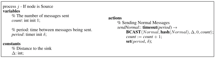
processj- If node is Source variables

% The number of messages sent count: int init 1;

% period: time between messages being sent. period: timer init ;

constants

% Distance to the sink : int;

actions

% Sending Normal Messages sendNormal::timeout(period)!

BCASThN ormal,hash(N ormal), ,0,counti; count:=count+ 1;

set(period, );

Algorithm 1. SLP Algorithm - Real Source Node.

[image:9.595.101.479.559.663.2]

(10)

SLP to the convergecast algorithm. It was previously observed, in [3], that using a flooding algorithm as convergecast provides no SLP. In this work, we thus use the flooding algorithm as baseline convergecast protocol, and enhance it with our proposed heuristics for SLP. Thus, any improvement in the level of SLP will be due to the proposed heuristics (and not due to the convergecast protocol). We build our heuristic on top of a simple flooding algorithm (as convergecast), which the real source uses to send messages to the sink. However, our proposed heuristic will work with any convergecast protocol [20, 22].

The convergecast algorithm that is used in this paper is implemented as follows : The (real) source (Algorithm 1) periodically generates an application message, as a result of detecting the asset, and broadcasts it to every normal node (Algorithm 3) in its neighbourhood (through actionsendNormal). The message contains asequence number, denoted bycount, and a field, calledhop, that keeps track of the (hop) distance the message has travelled. Thehopvalue is initialised to 0 by the real source node. The period between the source generating each application message as a result of the detection is application-dependent, and the period is denoted by . The message also contains a hash so that nodes can detect whether they have previously seen the message.

When a normal node receives the normal message, it executes the actionreceiveNormal, and

checks if the message is new, i.e., whether or not it has previously seen the same sequence number. If it is new, then the node increments thehopvalue by one and broadcasts the message. This process is repeated until the message reaches the sink. The value of thehopcount at the sink represents the distance of the real source from the sink.

5.3. Algorithm for Fake Sources

The algorithm needed to select permanent and temporary fake sources is heavily linked to the network configuration. Also, since the source node sends application messages at a given rate, then the fake sources (temporary and permanent) needs to send messages at a given rate, as well over their duration as fake sources. Since messages from the source node will draw the attacker closer to the source, and message from fake sources will draw the attacker away from the source node, we expect that the rate at which fake sources send fake messages to be strictly greater than that of the source node, so that the overall movement of the attacker is away from the source, i.e., the more fake messages an attacker hear, the further he will go from the source. Hence, we will also investigate the impact of thefake message periodon the level of SLP that is imparted.

In the network, there will be four types of nodes: (i) source node, (ii) sink, (iii) normal nodes and (iv) fake sources, and there will be three different types of messages, namely: normal messages, fake messages and protocol messages. Each node will typically send and/or receive these types of messages, giving rise to twelve possible classes of methods (or actions). For example, a normal node receiving a protocol message or a fake source receiving a fake message and so on, and each of these twelve possible classes of events will cause the algorithm to perform some action. It was mentioned in Section 4.1 that a fake source algorithm consists of a fake source selection algorithm and a message relaying algorithm. However, since we are interested in the selection of temporary and permanent fake sources, and the execution of fake sources, we will focus on the parts of the fake source algorithm that achieve these (i.e., we will focus on the fake source selection algorithm and we will omit unnecessary details about message relaying - for example, we will not explain what happens when the sink receives a fake message).

In general, the algorithm for fake sources work as follows:

1. The source node periodically generates ahNormalimessage, which is flooded through the

network, over a given time. In our paper, the time is simulation time.

2. As normal nodes receive their firsthNormalimessage they set their source distance as the number of hops that message had travelled.

3. When the sink node receives their firsthNormalimessage, it broadcasts anhAwayimessage. 4. ThishAwayimessage is flooded to the entire network and contains network knowledge (such

as the sink-source distance).

5. The nodes that receive thehAwayimessage that are one hop from the sink become

(11)

6. These temporary fake sources broadcast hFakei messages every given period for a given duration.

7. Once that duration is up the temporary fake sources broadcast a hChoosei message and

become normal nodes again.

8. When a normal node receives ahChooseimessage it either becomes a temporary or permanent

fake source, depending on if the permanent flag is set.

9. This fake source will start broadcastinghFakeimessage, if it is permanent it will not stop doing so.

5.3.1. Sink Receives ahNormaliMessage

The algorithm for selecting (permanent and temporary) fake sources starts once the sink receives the first normal message from the source. Upon receiving this, the sink executes Algorithm 2. Since the sink may receive the same message via different routes (since the message was flooded by the source), it keeps track of the message so that the message is not processed again. Then, the sink sends a special message, calledhAwayi, that contains some network information. This network information is necessary to select temporary and permanent fake nodes. At this point, no fake source (temporary or permanent) exists yet in the network.

% ReceivinghNormaliMessage

SinkReceiveNormal::rcvhN ormal, hash, ssd, hop, count, maxHopi ! if(hash2/messages)then

messages:=messages[{hash};

sink source:=min?{ sink source, hop+ 1};

if(¬sinkSent)then sinkSent:=T rue; A:=GetAlgorithm();

BCASThAway,hash(Away), sink source,0, maxHop,AiSenseRepeat(3)in2;

fi; fi;

Algorithm 2. SLP Algorithm - Sink ReceiveshNormaliMessage

5.3.2. Normal Node ReceiveshNormaliMessage

When a normal node receives ahNormali(application) message, it performs the following action, as in Algorithm 3. If a normal node believes it lies on the periphery of the network (maxHop 1<

firstHop), then itmaybecome a permanent fake source (whenisPermis True). Only nodes with the

isPermflag set are candidates for permanent fake sources. This is so as, given the configurations we consider in this paper, a node on the periphery of the network is always likely to be the furthest

from the actual source (see Figure 1). The variable maxHopkeeps track of the distance of the

furthest nodes from the real source known so far to a noden, and if that distance is greater thann’s

own distance from the real source, thenncannot become a permanent fake source. The premise for

having permanent fake sources on the periphery of the network is so that they can permanently keep the attacker away from the source node, i.e., until the safety period has elapsed.

However, at this point, the selection of permanent fake sources are not fully decided for the following reason: because of possible message collisions, a normal node may receive a normal

message via a long route, and may wrongly believe (by comparing its firstHop value against

maxHop) that it lies of the network periphery. This tagging will be confirmed (when the node is selected as a permanent node) or rescinded later in the protocol.

5.3.3. Normal Node ReceiveshAwayimessage

Now, when a normal node receives thehAwayimessage (see Algorithm 4), it checks if theDSink

value is 0. If it is, then the node becomes a temporary fake source with duration⌧, which is a

(12)

% ReceivinghNormaliMessage

NormalReceiveNormal::rcvhN ormal, hash, ssd, hop, count, maxHopi ! if(firstHop=? _maxHop 1>firstHop)then

isPerm:=F alse; fi;

sink source:=min?{ sink source, ssd};

if(hash2/messages)then

messages:=messages[{hash}; if(count = 1)then

firstHop, isPerm:=hop+ 1, T rue; fi;

source:=min?{ source, hop+ 1};

BCASThN ormal, hash, sink source, hop+ 1, count,max{firstHop, maxHop}i;

fi;

Algorithm 3. SLP Algorithm - Normal Node ReceiveshNormaliMessage

The reason we choose to elect nodes at one hop to become fake sources is so that the attacker can be kept from getting closer to the asset as soon as possible.

% ReceivinghAwayiMessage

NormalReceiveAway::rcvhAway, hash, ssd, Dsink, maxHop, algorithmi ! if(firstHop=? _maxHop 1>firstHop)then

isPerm:=F alse; fi;

if(algorithm6=?)then A:=algorithm; fi;

if(hash2/messages)then

messages:=messages[{hash};

sink:=min?{ sink, Dsink};

if(Dsink= 0)then

BecomeFakeSource(duration=⌧);

% Create a new hash otherwise future choose messages will fail to work BCASThAway,hash(Away), sink source, Dsink+ 1,

max{firstHop, maxHop},AiSenseRepeat(2); else

BCASThAway, hash, sink source, Dsink+ 1,

max{firstHop, maxHop},AiSenseRepeat(2); fi;

fi;

Algorithm 4. SLP Algorithm - Normal Node ReceiveshAwayiMessage

5.3.4. Temporary Fake Source Executes and Ends

When a node has been selected as a temporary fake source, it generates fake messages (which are identical in size to real messages sent by the real source, hence indistinguishable to an attacker). The values that are carried in the fake messages depend heavily on the network configuration.

For the Source Corner, Sink Corner and Further Sink Corner configurations, some network information piggybacks within the fake messages but, most importantly, the timer is set again for

the fake source to send messages after a Fi period, which is a parameter of the heuristic. The

only difference between the algorithm needed for the Source Corner and the other two is that some checks are performed (see Algorithm 5).

When the duration of the temporary fake source elapses (see Algorithm 6), it sends ahChoosei

message, and becomes a normal node again, i.e., it stops sending fake messages.

5.3.5. Normal Node ReceiveshChooseiMessage

When a normal node receives ahChooseimessage from a previously temporary fake source (see

(13)

SendinghFakeiMessage When Configuration is SourceCorner FSSendFake::timeout(period)!

BCASThF ake,hash(F ake), sink source,duration=1, f irstHop, source, sink, ji;

if(duration=1 ^¬isPerm)then set(duration,0);

else

set(period, Fi); fi;

SendinghFakeiMessages when Configuration is SinkCorner and FurtherSinkCorner FSSendFake::timeout(period)!

BCASThF ake,hash(F ake), sink source,duration=1, f irstHop, source, sink, ji;

set(period, Fi);

Algorithm 5. Temporary Fake Source Executes

% Stop SendinghFakeiMessages after the given duration FSStopSending::timeout(duration)!

BCASThChoose,hash(Choose), sink source, hop+ 1,firstHop,AiSenseRepeat(3);

BecomeNormal();

Algorithm 6. Temporary Fake Source Stops Executing

source, and its duration is set to1. Otherwise, it becomes a temporary fake source with duration

⌧. Observe that the algorithm for handling the hChoosei message is configuration-dependent.

Specifically, for the SourceCorner configuration, a node cannot become a temporary fake source if the following condition holds: ( source3₄ sink source), i.e., it is less than3₄ the network radius to the source. This is due to energy optimisation reasons. For the SinkCorner and FurtherSinkCorner configurations, the condition is (1

2 the network radius - 1).

Implementation Issues: As mentioned before, the structure of the messages sent by the temporary and permanent fake sources are identical to those sent by the real source. The only difference is in the payload, where in the case of the fake sources, the payload is random. Based on this, we assume an attacker cannot distinguish between a real message and a fake one. Note that, as our assumption is that real messages are encrypted, so are the fake messages. This means that only legitimate nodes can read the fake messages. However, when there is more than one fake source operating, this may result in a legitimate intermediate node dropping messages from two different fake source nodes on the basis that the messages were identical.

6. EXPERIMENTAL SETUP

In this section we describe the simulation environment and protocol configurations that were used to generate the results presented in Section 7.

6.1. Simulation Environment

(14)

ReceivinghChooseiMessage when configuration is SinkCorner and FurtherSinkCorner NormalReceiveChoose::rcvhChoose, hash, ssd, hop, maxHop, algorithmi !

if(firstHop=? _maxHop 1>firstHop)then isPerm:=F alse;

fi;

if(hash2/messages^¬seenPerm^

¬( sink source6=? ^ source1₂ sink source 1))then

messages:=messages[{hash}; if(isPerm)then

BecomeFakeSource(duration=1); else

BecomeFakeSource(duration=⌧); fi;

fi;

ReceivinghChooseiMessage when configuration is SourceCorner

NormalReceiveChoose::rcvhChoose, hash, ssd, hop, maxHop, algorithmi ! if(firstHop=? _maxHop 1>firstHop)then

isPerm:=F alse; fi;

if(hash2/messages^¬( sink source6=? ^ source3₄ sink source))then

messages:=messages[{hash}; if(isPerm)then

BecomeFakeSource(duration=1); else

BecomeFakeSource(duration=⌧); fi;

fi;

Algorithm 7. SLP Algorithm - Normal Node ReceivinghChooseiMessage

been developed for sensor networks. JProwler was chosen due to its java-based implementation. On the other hand, simulators such as NS2 use different MAC protocols that are not very suited to sensor networks.

6.2. Network Setup

A square grid network layout of sizen⇥nwas used in all experiments, wheren2{11,15,21,25}, i.e., networks with 121, 225, 441 and 625 nodes respectively. A single source node generated normal application messages and a single sink node collected messages. The source and sink nodes were distinct. The period between messages being generated from the real source was varied. Simulations were run for every grid configuration, varying the network size, source rate, the fake source rate and the temporary fake source duration.

6.3. Protocol Configuration

The flooding protocol was used as a baseline against which the SLP protocol was measured. In this paper, we are interested in the impact two protocol parameters have on the level of SLP. These are:

1. The duration⌧ia temporary fake sourcenisends fake messages.

2. The period Fibetween which a temporary or permanent fake sourcenisends messages.

(15)

[image:15.595.124.453.127.329.2]

Table II. Safety Periods for the SourceCorner configuration for GRID networks

Size Period Source-Sink Received Average Time Safety Period

(seconds) Distance (hop) (%) Taken (seconds) (seconds)

11 1 10 84 16.79 33.58

11 0.5 10 82 8.45 16.90

11 0.25 10 80 4.50 8.99

11 0.125 10 44 4.70 9.41

15 1 14 84 24.82 49.63

15 0.5 14 83 12.43 24.85

15 0.25 14 80 6.64 13.29

15 0.125 14 43 7.23 14.47

21 1 20 84 36.76 73.52

21 0.5 20 83 18.37 36.74

21 0.25 20 81 9.89 19.78

21 0.125 20 43 11.45 22.90

25 1 24 85 44.90 89.80

25 0.5 24 83 22.34 44.68

25 0.25 24 81 12.17 24.34

25 0.125 24 43 14.26 28.52

fake messages as well as the rate at which the real source sends normal messages by changing the period between being sent. For the real source, the message period used were 1, 0.5 and 0.25 seconds per message, whereas the message periods for the fake sources, in general, were 0.5, 0.25 and 0.125 seconds per message. We also never ran simulations where the message rate of the real source is higher than that of the fake source, since the capture ratio will, in general, be close to 100% (as the attacker is “attracted” faster towards the real source than towards the fake source). Thus, a protocol configuration is a 3-tuple (real source period2{1,0.5,0.25}, fake source period 2{0.5,0.25,0.125}, fake source duration2{1,2,4}).

6.4. Safety Period

A concept called safety period was introduced in [3] to capture the number of messages that has to be sent by the real source before it gets detected. In general, for a high level of SLP, the safety period should ideally be very high, i.e., a high number of messages need to be sent by the source node before it is captured. However, the problem with this definition, from a simulation perspective, is to determine when the simulation should stop, i.e., if a very large number of messages is needed, then the simulation time becomes very long.

Thus, we use an alternative, but complementary, definition for safety period [12] which is time-based: for each network size and source rate, using flooding (since it provide no SLP), we calculate the average time it takes an attacker to detect the real source (i.e., capture the asset). This time is called the capture time. Since the SLP algorithm will make it more difficult for an attacker to reach the source node, i.e., capture the asset, we set the safety period to twice the capture time. The reason for using this definition of safety period is that it bounds the simulation time. Intuitively, the safety period provides the attacker a time upper bound during which he can reach the source node. Since, in the original SLP paper, the asset were endangered species, the safety period captures the time during which the animal or asset will be at the same location before it moves away.

(16)

[image:16.595.125.452.127.331.2]

Table III. Safety Periods for the SinkCorner configuration for GRID networks

11 1 10 56 15.76 31.53

11 0.5 10 56 7.93 15.87

11 0.25 10 55 4.14 8.29

11 0.125 10 36 4.58 9.16

15 1 14 57 23.64 47.29

15 0.5 14 57 11.96 23.91

15 0.25 14 56 6.20 12.39

15 0.125 14 34 7.46 14.92

21 1 20 59 35.50 71.00

21 0.5 20 58 17.84 35.69

21 0.25 20 56 9.42 18.85

21 0.125 20 33 12.32 24.65

25 1 24 59 43.54 87.08

25 0.5 24 57 21.86 43.73

25 0.25 24 57 11.60 23.19

[image:16.595.125.453.355.558.2]

25 0.125 24 33 15.94 31.87

Table IV. Safety Periods for the FurtherSinkCorner configuration for GRID networks

11 1 14 57 23.71 47.42

11 0.5 14 58 11.95 23.90

11 0.25 14 56 6.23 12.45

11 8 14 34 7.19 14.37

15 1 22 59 39.73 79.46

15 0.5 22 58 19.87 39.75

15 0.25 22 56 10.53 21.07

15 8 22 33 12.95 25.89

21 1 34 59 63.89 127.79

21 0.5 34 58 32.05 64.09

21 4 34 57 17.24 34.48

21 8 34 32 22.34 44.67

25 1 42 59 80.34 160.69

25 0.5 42 58 40.25 80.50

25 0.25 42 57 21.92 43.83

25 0.125 42 32 28.53 57.07

6.5. Simulation Experiments

(17)

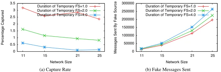
SourceCorner - Duration

0 0.1 0.2 0.3 0.4 0.5 0.6 0.7 0.8 0.9

11 15 21 25

Percentage Captured

Network Size Duration of Temporary FS=1.0 Duration of Temporary FS=2.0 Duration of Temporary FS=4.0

(a) Capture Rate

0 50000 100000 150000 200000 250000 300000

11 15 21 25

Messages Sent By Fake Source

[image:17.595.106.467.126.259.2]

(b) Fake Messages Sent

Figure 2. Varying the Duration of Temporary Fake Sources for the SourceCorner configuration. Parameters: Source Period=1.0 sec, Fake Source Period=0.25 sec

Also, every temporary fake source will have the same duration and fake source period. Given the number of nodes in the network, varying these parameters individually would give rise to a massively large number of experiments to run. The thrust of the paper is to determine whether, varying the duration and (fake) message periods, affect the level of SLP of the network.

7. RESULTS

In this section, we present the results of our simulation experiments under various protocol parameterisations.

7.1. Metrics

We use the capture ratio metric to indicate the level of SLP. The capture ratio metric is calculated as the ratio of the number of runs in which the source is captured within the safety period to the total number of runs. If the capture ratio is 0%, then it means that the SLP is maximal, whilst the SLP is minimal if the capture ratio is 100%. Further, we assume that the durations⌧ito be equal for all temporary fake sources, and the message period Fito be equal for all temporary fake sources.

7.2. Impact of Temporary Fake Source Duration on SLP

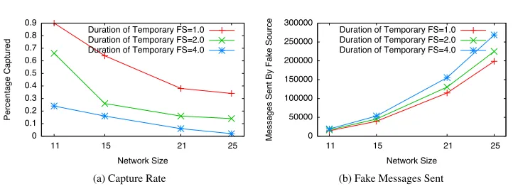
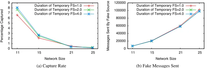
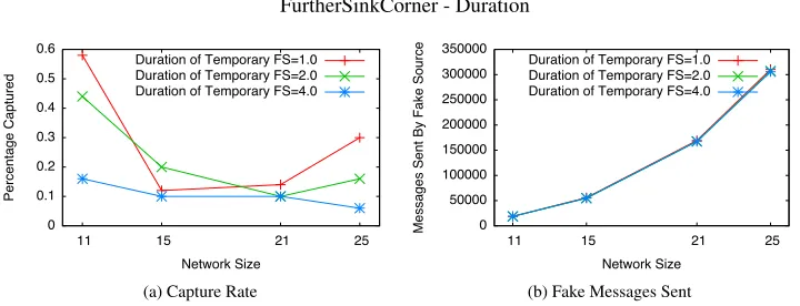
In this section, we investigate the impact of fake source duration on the level of SLP imparted by the proposed heuristic. Specifically, we wish to understand how the duration during which a fake source sends fake messages affect SLP. Intuitively, the higher the duration, the higher the chance of the attacker being “pulled back”, decreasing the capture ratio. We investigate the impact on the three different network configurations.

From the graphs on duration (Figures 9-14), we observe that, in general, an increase in the duration during which a node acts as a fake sources results in a lower capture ratio, hence higher level of SLP. It is worth noting that near optimal privacy is attainable, i.e., capture ratio of almost 0 (see Figures 9 and 10). When only flooding is used, the capture ratio is 100% [3]. This demonstrates the high level of privacy imparted by the heuristics proposed here as, in general, the capture ratio is kept very low (7%and, in most cases,3%).

7.3. Impact of Fake Message Periods on SLP

(18)

SourceCorner - Duration 0 0.5 1 1.5 2 2.5

11 15 21 25

Percentage Captured

(a) Capture Rate

0 50000 100000 150000 200000 250000

11 15 21 25

[image:18.595.107.468.135.257.2]

Figure 3. Varying the Duration of Temporary Fake Sources for the SourceCorner configuration. Parameters: Source Period=1.0 sec, Fake Source Period=0.5 sec

SinkCorner - Duration

0 0.5 1 1.5 2 2.5

11 15 21 25

Percentage Captured

(a) Capture Rate

0 20000 40000 60000 80000 100000 120000 140000 160000

11 15 21 25

[image:18.595.107.466.309.434.2]

Figure 4. Varying the Duration of Temporary Fake Sources for the SinkCorner configuration. Parameters: Source Period=1.0 sec, Fake Source Period=0.25 sec

SinkCorner - Duration

0 1 2 3 4 5 6 7 8 9

11 15 21 25

Percentage Captured

(a) Capture Rate

0 20000 40000 60000 80000 100000 120000

11 15 21 25

Figure 5. Varying the Duration of Temporary Fake Sources for the SinkCorner configuration. Parameters: Source Period=1.0 sec, Fake Source Period=0.5 sec

[image:18.595.108.467.490.608.2]

(19)

FurtherSinkCorner - Duration 0 0.1 0.2 0.3 0.4 0.5 0.6

11 15 21 25

Percentage Captured

(a) Capture Rate

0 50000 100000 150000 200000 250000 300000 350000

11 15 21 25

[image:19.595.107.467.120.258.2]

Figure 6. Varying the Duration of Temporary Fake Sources for the FurtherSinkCorner configuration. Parameters: Source Period=1.0 sec, Fake Source Period=0.25 sec

FurtherSinkCorner - Duration

0 0.2 0.4 0.6 0.8 1 1.2 1.4 1.6 1.8

11 15 21 25

Percentage Captured

(a) Capture Rate

0 20000 40000 60000 80000 100000 120000 140000 160000 180000 200000

11 15 21 25

[image:19.595.107.467.320.440.2]

Figure 7. Varying the Duration of Temporary Fake Sources for the FurtherSinkCorner configuration. Parameters: Source Period=1.0 sec, Fake Source Period=0.5 sec

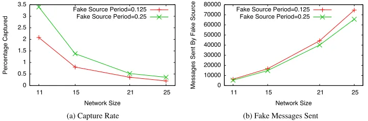
SourceCorner - Fake Source Rate

0 0.1 0.2 0.3 0.4 0.5 0.6 0.7

11 15 21 25

Percentage Captured

Network Size Fake Source Period=0.125

Fake Source Period=0.25 Fake Source Period=0.5

(a) Capture Rate

0 50000 100000 150000 200000 250000 300000

11 15 21 25

Network Size Fake Source Period=0.125 Fake Source Period=0.25 Fake Source Period=0.5

Figure 8. Varying the Fake Source Rate for the SourceCorner configuration. Parameters: Source Period=1.0 sec, Duration=4.0 sec

[image:19.595.107.467.505.623.2]

(20)

SourceCorner - Fake Source Rate 0 0.1 0.2 0.3 0.4 0.5 0.6

11 15 21 25

Percentage Captured

Fake Source Period=0.25

(a) Capture Rate

0 20000 40000 60000 80000 100000 120000 140000

11 15 21 25

Network Size Fake Source Period=0.125 Fake Source Period=0.25

[image:20.595.107.467.133.257.2]

Figure 9. Varying the Fake Source Rate for the SourceCorner configuration. Parameters: Source Period=0.5 sec, Duration=4.0 sec

SinkCorner - Fake Source Rate

0 1 2 3 4 5 6 7 8

11 15 21 25

Percentage Captured

(a) Capture Rate

0 20000 40000 60000 80000 100000 120000 140000 160000 180000

11 15 21 25

[image:20.595.107.467.321.439.2]

Figure 10. Varying the Fake Source Rate for the SinkCorner configuration. Parameters: Source Period=1.0 sec, Duration=2.0 sec

SinkCorner - Fake Source Rate

0 0.5 1 1.5 2 2.5 3 3.5

11 15 21 25

Percentage Captured

(a) Capture Rate

0 10000 20000 30000 40000 50000 60000 70000 80000

11 15 21 25

Figure 11. Varying the Fake Source Rate for the SinkCorner configuration. Parameters: Source Period=0.5 sec, Duration=2.0 sec

8. DISCUSSION

[image:20.595.106.467.505.624.2]

(21)

FurtherSinkCorner - Fake Source Rate

0 0.2 0.4 0.6 0.8 1 1.2 1.4 1.6 1.8

11 15 21 25

Percentage Captured

(a) Capture Rate

0 50000 100000 150000 200000 250000 300000 350000

11 15 21 25

[image:21.595.107.466.130.258.2]

Figure 12. Varying the Fake Source Rate for the FurtherSinkCorner configuration. Parameters: Source Period=1.0 sec, Duration=4.0 sec

FurtherSinkCorner - Fake Source Rate

0 0.1 0.2 0.3 0.4 0.5 0.6 0.7 0.8 0.9

11 15 21 25

Percentage Captured

(a) Capture Rate

0 20000 40000 60000 80000 100000 120000 140000 160000

11 15 21 25

Figure 13. Varying the Fake Source Rate for the FurtherSinkCorner configuration. Parameters: Source Period=0.5 sec, Duration=4.0 sec

8.1. Alternative Topologies and Configurations

In this paper, we have focused on three different configurations of the grid topology. However, if a WSN can be divided into four quadrants such that all of them are similar in size/density, we conjecture that our fake sources protocol will work. However, partitioning the network in such a way is not always possible. In this case, new heuristics are needed. Specifically, new algorithms for generating fake sources will need to be developed for each configuration of the network. Our current work is focusing on different network topologies, namely rings and circles.

8.2. Energy Issues

It was argued in [3] that the fake source technique may not be energy efficient. However, as explained earlier, the two parameters of the heuristics, namely fake source message period and fake source duration can be used to fine tune the energy expenditure of the protocol. For example, setting the fake source duration parameter to be small will likely cause a small energy usage, as will the fake source message period. However, the energy savings will come at the expense of lower SLP. Thus, there is a tradeoff to be made, as can be seen in Figures 9–20, in that higher duration and lower fake message periods lead to higher SLP. We have observed combinations of values for fake source duration and fake message periods that result in near optimal SLP.

[image:21.595.107.467.316.436.2]

(22)

SourceCorner - Duration 0 0.1 0.2 0.3 0.4 0.5 0.6 0.7 0.8 0.9

11 15 21 25

Percentage Captured

(a) Capture Rate

0 50000 100000 150000 200000 250000 300000

11 15 21 25

[image:22.595.106.467.137.256.2]

Figure 14. Varying the Duration of Temporary Fake Sources for the SourceCorner configuration. Parameters: Source Period=1.0 sec, Fake Source Period=0.25 sec, Pr(TFS)=100%

0 0.5 1 1.5 2 2.5 3 3.5

11 15 21 25

Percentage Captured

(a) Capture Rate

0 50000 100000 150000 200000 250000 300000

11 15 21 25

[image:22.595.107.468.313.432.2]

0 2 4 6 8 10 12 14 16

11 15 21 25

Percentage Captured

(a) Capture Rate

0 50000 100000 150000 200000 250000 300000

11 15 21 25

[image:22.595.107.467.490.608.2]

(23)

9. CONCLUSION

This paper explored the fake source technique for providing SLP in a WSN. Specifically, this paper has provided a novel formalisation of the fake source selection problem and has shown the problem to be NP-complete. Two important parameters, namely fake message rates and fake source duration, have been identified that impact on the achievable levels of SLP. Further, heuristics for solving the SLP problem for various network configurations were proposed and their efficiency demonstrated through extensive simulation.

In future work it would be desirable to develop new heuristics to address the SLP problem for different topologies and network configurations. It would also be informative to consider alternative attacker models, particularly in the contexts of the heuristics developed in this paper.

REFERENCES

1. Ceriotti M, et al. Monitoring heritage buildings with wireless sensor networks: The torre aquila deployment. Proceedings of Information Processing in Sensor Networks, 2009; 277–288.

2. Mainwaring A, Polastre J, Szewczyk R, Culler D. Wireless sensor networks for habitat monitoring.Proceedings of the First ACM International Workshop on Wireless Sensor Networks and Applications, 2002.

3. Kamat U, Zhang Y, Ozturk C. Enhancing source-location privacy in sensor network routing.Proceedings of the 25th IEEE International Conference on Distributed Computing Systems, 2005; 599–608.

4. Perrig A, Stankovic J, Wagner D. Security in wireless sensor networks.Communications of the ACM - Special Issue on Wireless Sensor NetworksJune 2004;47(6):53–57.

5. Lamport L, Shostak R, Pease M. The byzantine generals problem.ACM Transactions on Programming Languages and SystemsJuly 1982;4(3):382–401.

6. Nesterenko M, Tixeuil S. Discovering network topology in the presence of byzantine faults.IEEE Transactions on Parallel and Distributed SystemsDecember 2009;20(12):1777–1789.

7. Avramopoulos IC, Kobayashi H, Wang R, Krishnamurthy A. Highly secure and efficient routing.Proceedings of the 23rd Annual Joint Conference of the IEEE Computer and Communications Societies, 2004; 197–208. 8. Mehta K, Liu D, Wright M. Location privacy in sensor networks against a global eavesdropper.Proceedings of the

15th IEEE International Conference on Network Protocols, 2007; 314–323.

9. Armenia S, Morabito G, Palazzo S. Analysis of location privacy/energy efficiency tradeoffs in wireless sensor networks.Proceedings of the 6th International IFIP-TC6 Networking Conference on Ad Hoc and Sensor Networks, Wireless Networks, Next Generation Internet, 2007; 215–226.

10. Lee SW, Park YH, Son JH, Seo SW, Kang U, Moon HK, Lee MS. Source-location privacy in wireless sensor networks.Korea Institute of Information Security and Cryptology JournalApril 2007;17(2):125–137.

11. Yao J, Wen G. Preserving source-location privacy in energy-constrained wireless sensor networks.Proceedings of the 28th International Conference on Distributed Computing Systems Workshops, 2008; 412–416.

12. Jhumka A, Leeke M, Shrestha S. On the use of fake sources for source location privacy: Trade-offs between energy and privacy.The Computer JournalJune 2011;54(6):860–874.

13. Ozturk C, Zhang Y, Trappe W. Source-location privacy in energy-constrained sensor network routing.Proceedings of the 2nd ACM Workshop on Security of Ad Hoc and Sensor Networks, 2004; 88–93.

14. Tian H, Shen H, Matsuzawa T. Random walk routing in wsns with regular topologies.Journal of Computer Science and Technology2006;21(4):496–502.

15. Mabrouki I, Lagrange X, Froc G. Random walk based routing protocol for wireless sensor networks.Proceedings of the 2nd international conference on Performance Evaluation Methodologies and Tools, 2007.

16. Palmieri F, Castiglione A. Condensation-based routing in mobile ad-hoc networks.Mobile Information Systems June 2012;8(3):199–211.

17. Deng J, Han R, Mishra S. Countermeasures against traffic analysis attacks in wireless sensor networks.Proceedings of the 1st International Conference on Security and Privacy for Emerging Areas in Communications Networks, 2005; 113–126.

18. Ouyang Y, Le Z, Liu D, Ford J, Makedon F. Source location privacy against laptop-class attacks in sensor networks. Proceedings of the 4th International Conference on Security and Privacy in Communication Networks, 2008; 22– 25.

19. Kamat P, Xu W, Trappe W, Zhang Y. Temporal privacy in wireless sensor networks: Theory and practice.ACM Transactions on Sensor NetworksNovember 2009;5(4):24 (Article 28).

20. Jhumka A. Crash-tolerant collision-free data aggregation scheduling in wireless sensor networks.Proceedings 29th IEEE Symposium on Reliable Distributed Systems, 2010; 44–53.

21. Benenson Z, Cholewinski PM, Freiling FC.Wireless Sensor Network Security, chap. Vulnerabilities and Attacks in Wireless Sensor Networks. IOS Press, 2008; 22–43.