Topological interactions in ring polymers

(1)

University of Warwick institutional repository:

http://go.warwick.ac.uk/wrap

A Thesis Submitted for the Degree of PhD at the University of Warwick

http://go.warwick.ac.uk/wrap/77355

This thesis is made available online and is protected by original copyright.

Please scroll down to view the document itself.

(2)

Topological Interactions in Ring Polymers

by

Davide Michieletto

A Thesis submitted to the

University of Warwick

for the degree of

Doctor of Philosophy in Physics and Complexity Science

University of Warwick, Department of Physics and Centre for Complexity Science

(3)

Ringraziamenti

Acknowledgements

Vorrei ringraziare Stefania, anche se mai abbastanza, per tutti i sacrifici e le diffi-coltà che ha condiviso con me in questi quattro anni: ogni piccolo o grande momento di tristezza è servito a renderci ancor più risoluti ed è stato ricompensato con sod-disfazioni ugualmente grandi. Grazie per i momenti felici, per aver detto s`ı e per i “com’è andata” a fine giornata: Spero di sentirli ogni giorno per molti anni ancora. Vorrei ringraziare la mia famiglia: i miei genitori Elena e Daniele, nonni Berto, Anna e Palmira, zii Dante, Wally, Bruno e Alfreda, cugini Roberto, Barbara e Luca; ed anche Sonia, Domenico, Andrea e Bruna. Non c’è riposo più sereno che nel calore di chi ti vuole bene e ti fa sentire a casa, e non c’è persona più ingrata di colui che non lo apprezza.

I would like to thank the many old friends with whom we have been sharing experiences and emotions during the past ten years: Anna and Riccardo for always being in each-other thoughts even though being miles apart, Elisa for being a sweet friend, Anna and Stefano for their inspiring dedication to each-other, Alessio for his uniqueness, Bisi, Sara, Cece, Cicci, Zakk and Tommy for their precious friendship. We feel honoured to be part of such strong group of brilliant persons that has been scattered across Europe and nonetheless managed to remain whole.

I would like to thank the new friends we made in England: Peter and Jen for their kindness and welcoming hearts, Dario and Tom for their (too) many talents, Ellen for her teasing and Quentin for having patiently introduced us to life in Eng-land. Thanks also to Dayal, Simone and Marco: the friends we would turn to when felt like missing home.

Finally, I would like to thank who supervised me during these years and to whom I could turn to when in need of sharing ideas and seeking inspiration: Matthew, Gareth, Enzo and Davide. You have been not only an essential part of my academic life, but each one of you has also taught me something that will make me a better man, and for that I will be forever grateful.

(6)

Declaration

This Thesis is submitted to the University of Warwick in support of my application for the degree of Doctor of Philosophy. It has been composed by myself and has not been submitted in any previous application for any degree.

The work presented (including data generated and data analysis) was carried by the author.

Parts of this Thesis have been published by the author:

(1) D. Michieletto, D. Marenduzzo, E. Orlandini, G. P. Alexander, M. S. Turner, Threading Dynamics of Ring Polymers in a Gel, ACS Macro Lett.,

3, 255-259 (2014)

(2) D. Michieletto, D. Marenduzzo, E. Orlandini, G. P. Alexander, M. S. Turner,Dynamics of Self-Threading Polymers in a Gel, Soft Matter,10, 5936-5944 (2014)

(3) D. Michieletto, E. Orlandini, M. S. Turner, Rings in Random Environ-ments: Sensing Disorder Through Topology, Soft Matter,11, 1100-1106 (2015)

(4) D. Michieletto, D. Marenduzzo, E. Orlandini, Is the Kinetoplast DNA a Percolating Network of Linked Rings at its Critical Point?, Phys. Biol., 12, 036001 (2015)

(5) D. Michieletto, D. Marenduzzo, M. S. Turner,Topology Regulation during Replication of the Kinetoplast DNA,sub judice (arXiv:1408.4237)

(6) D. Michieletto, D. Marenduzzo, E. Orlandini,Topological Patterns in Two-dimensional Gel Electrophoresis of DNA Knots, Proc. Natl. Acad. Sci. USA,

112(40), E5471-E5477 (2015)

(7)

CONTENTS v

Below, I will describe (i) how the material published in the aforementioned papers is reported and distributed in the Thesis Chapters and (ii) the respective contribu-tion of the authors to the papers:

The material published in paper (1) is described in Chapter 4 of the Thesis. The material of paper (2), although similar in spirit to paper (1), has been described in Appendix B of this Thesis. This choice reflects the different numerical methods used to simulate the systems considered. The goals and physical ideas behind these pa-pers (and of Chapter 4 and Appendix B), have been inspired by my supervisor Prof. Matthew Turner. At the start of my PhD I did not possess the numerical expertise needed to set up these complex simulations. I therefore sought the expertise of my external supervisor Dr. Davide Marenduzzo and of my former MSc supervisor Prof. Enzo Orlandini, who suggested the right numerical tools to use. Throughout the project I also sought the expertise of Dr. Gareth Alexander, who helped with the formal definitions of the topological operations and algorithms needed to obtain our novel findings. I have run the simulations and analysed the data, while all authors have contributed to write the paper.

The content of papers (4) and (5) is described in Chapter 5 and Appendix C. The idea behind these papers came to me when looking for an example of topologically linked rings in biology. Once again, I sought the collaboration and expertise of Dr. Marenduzzo and Prof. Orlandini to define the coarse-grained numerical model that could best reproduce the biological system under study. An analytical attempt to describe this system (paper (5)) was originated while I was describing paper (4) to Prof. Turner.

(8)

Abstract

R

ing polymers offer a richness of behaviours that are of broad interest and

have deep consequences in many fields of Science. In this Thesis I in-vestigate some general and universal properties, i.e. independent of the chemical nature of the polymers, emerging from systems made of a collection of rings. These will be studied by using methods of equilibrium and non-equilibrium Statis-tical Mechanics together with Molecular Dynamics and Monte Carlo simulations of coarse-grained models for the systems under investigation. Within these frameworks, important questions regarding the macroscopic behaviour of ring-shaped polymers have yet to find a satisfactory answer. The work presented in this Thesis finds its principal motivations in problems arising in Material Science, the so called “melt” of rings, and in Biology, such as the organisation of mitochondrial DNA in some organisms and the mechanisms governing the electrophoretic separation of DNA samples in gels. There are several theoretical challenges in these fields which repre-sent state-of-the-art scientific research and whose partial answers are provided in the work presented in this Thesis. One of the major achievements of the work presented is the general understanding of the role played by topological properties, i.e. those invariant under smooth deformations of the polymer contour, on the macroscopic behaviour of the investigated systems. Finally, the conclusions drawn from the pre-sented work can have important scientific consequences as they may ultimately lead to a more complete understanding of complicated issues in Biology and to the design of next-generation soft materials.

(9)

List of Symbols

¯

ρp Percolation monomer density for a system of linkable rings confined in a box. The estimated percolation density is denoted asρp.

β “Surface exponent” relating the number of beads that are in contact with any other bead to the polymer length.

η Solution viscosity.

γ “Contact exponent” regulating the probability of two parts of the same chain,

ssegments apart, to be near one another.

hki Average network valence or mean vertex degree.

hli Average fraction of linearised mini-circles.

µ Mobility of an object dragged by an external forceF through a fluid with a stationary velocityv.

µD Differential mobility, i.e. the change in mobility in response to a change in the field strength.

ν Scaling exponent relating the spatial size of a polymer to its polymerisation index.

φ Volume fraction.

ΦM/D/T Fraction of monomers (one ring), dimers (two linked rings) and trimers (three linked rings) after digestion of a network of linked rings.

ρ Number density of polymer beads in the system. ρ∗ denotes the overlap number density.

σ Nominal diameter of a bead forming the polymers.

τdiam Polymer orientation time. Quantifies the time taken by a polymer to

re-arrange its conformation. It is obtained as a numerical time integral of the time-correlation functionCdiam(t) computed fromhd(t)·d(0)i, wheredis the

diameter vector of the polymer.

τrelax Polymer relaxation time, or time required for the centre of mass of a polymer

coil to diffuse a distance equal to the polymer average sizehR2_gi1/2_.

τRouse Rouse time, or time required for a bead forming a polymer to diffuse a

dis-tance equal to the polymer average sizehR2_gi1/2_.

ϕnc(t) Time correlation function for contiguous rings. The time-scale at which two

rings become non-contiguous is denoted byτnc.

(10)

CONTENTS viii

ξ Friction coefficient acting on a bead.

b1(G) First Betti number, or rank of the first homology group, of the graph G. It

measures the number of 1-dimensional holes in the graph.

c Concentration of polymeric mass in the system. c∗ denotes the overlap con-centration.

cp Fraction of explicitly immobilised (pinned) rings. The critical fraction at which the whole system displays a dynamical arrest is denoted withc†p.

DCM Diffusion coefficient of a polymer centre of mass.

dij Distance between bead iand beadj.

G(E,V) Directed graph composed by a set of verticesV and edgesE.

G(t) Stress relaxation modulus.

g1(t) Segmental mean square displacement of the beads, also identified withhδr2s(t)i.

g3(t) Mean square displacement of the centre of mass of the polymers, also

identi-fied withhδr2_CM(t)i.

L Linear dimension of the simulation box.

lp Persistence length of a semi-flexible polymer, i.e. the contour-length neces-sary for the tangent-tangent correlation to equal 1/e. The Kuhn length is denoted bylK and is twice the persistence length.

M Polymer number-weighted polymerisation index,i.e. number of beads form-ing the polymers.

m Mass of a bead.

Me Entanglement length, or number of beads at which a polymer starts to “feel” the presence of entanglement due to the neighbouring chains.

N Number of polymers in the system.

Pp(t) Threading time-correlation function. It quantifies the time required for the passive threadings observed at any time-step to disappear and release the constraint imposed.

PIJ(t) Matrix element identifying the “contact” of ring I and ringJ at timet.

pth Threading probability between two chains sharing the same gel unit cell.

Re,Rg End-to-end size and radius of gyration of a polymer coil.

S1(q) Static scattering function probed at length-scalesl= 2π/q.

Sc(q, t) Coherent scattering function probed at length-scalesl= 2π/q at timet.

T h(i, j;t) Matrix element which assumes value of unity if ring j is passing through ringi at timetand zero otherwise.

(11)

Io stimo più il trovar un vero, benché di cosa leggiera, che’l disputar lungamente delle massime questioni senza conseguir verità nissuna.†

G. Galilei

1

Introduction

R

ingpolymers are perhaps one of the last big mysteries in Polymer Physics.

Polymers are collections of simpler units, called monomers, which are nowa-days largely present in virtually any aspect of anyone’s life: in plastics, drugs and clothes. Perhaps most importantly, (bio-)polymers are at the heart of life itself, being inside any prokaryotic and eukaryotic cell under the form of DNA, RNA and proteins [Alberts et al., 2014].

The behaviour of linear polymers in solution is now understood in terms of the Rouse-Zimm and reptation models for dilute and concentrated conditions, respec-tively [de Gennes, 1979,Doi and Edwards, 1988,Rubinstein and Colby, 2003]. The behaviour of solutions of star, or quenched branched, polymers is also captured by describing the retraction of the arms similarly to that of the two terminal segments of linear polymers. On the contrary, the properties of un-linked and un-knotted ring polymers in solution present some big open questions and are far from being fully captured. Adding further topological constraints such as, linking between rings or knotting (see Fig. 1.1), complicates the picture even more. In these cases, in fact, the scientific community is not even equipped with the right mathematical tools to classify these objects: At present, a quantity does not exist that can unambiguously distinguish every knot or link [Adams, 1994].

Figure 1.1: Polymers with different topologies. From left to right: linear, star, branched (quenched), circular or ring, linked and knotted.

†I prefer finding something true, although of small importance, rather than keep debating on

the major issues failing to achieve any truth.

(12)

1. Introduction 2

Joining the two ends of an open chain would seem, at first sight, to be a rela-tively trivial change; In reality, it has a profound impact on the static and dynamic properties of a polymer [Bates and Maxwell, 2005]. This procedure in fact changes its topological state, i.e. the state that is preserved under smooth deformations of its contour, and introduces long-ranged constraints on the allowed conformations. The motion of ring polymers is rather different from that of linear polymers and this is entirely due to their lack of ends. While linear polymers explore the surrounding space by retracting and protruding their terminal segments, ring polymers have no ends to retract or protrude but, on the other hand, they can generate any number of temporary double-folded segments which can explore the space as if they were terminal segments. These conformations are sometimes referred to as “lattice ani-mals”, or annealed branched polymers, as the branch points are free to move along the polymer contour (see Fig. 1.2(a)). From this, one can understand that the lack-ing of ends does not necessarily reduce the ability of rlack-ing polymers to explore space but rather triggers completely different pathways through which rings re-arrange their shape. Ring polymers have, in some sense, a greater freedom of movement with respect to their linear or quenched branched polymers, although they suffer of much stronger topological constraints due to the fact that they have to preserve their topological state at all times. Because of all this, ring polymers in solution are, at present, a topic of intense debate and lively interest among the Polymer Physics community [Kapnistos et al., 2008,Halverson et al., 2011a,Mirny, 2011,Pasquino et al., 2013,Rosa and Everaers, 2014,Grosberg, 2014].

In spite of our difficulties in capturing their behaviour, ring polymers are abun-dant in Nature, who seems to have no difficulty at all to regulate their properties and topology, often in very delicate and life-depending conditions, such as in the case of bacterial DNA or inside the eukaryotic cell nucleus [Calladine et al., 1997, Al-berts et al., 2014]. For instance, bacterial DNA, which is circular, has to be kept un-knotted and un-linked at all times during mitosis; failing to do so would lead to the death of the organism as its replicated genetic material cannot be separated into the two daughter cells. DNA knots and links have been frequently observed in the genetic material of bacteria, viruses and eukaryotes, since their discovery in the late ’70s [Liu et al., 1976,Liu et al., 1981,Fairlamb et al., 1978], and because they are so ubiquitous, all organisms have developed special enzymes – called topoi-somerases [Berger et al., 1996] – whose function is to help untie DNA knots and links. This indicates how the topological regulation in systems of bio-polymers is a serious issue, and learning how Nature deals with it might provide us with fresh means to design next-generation soft materials or to understand and detect genetic diseases [Cavalli and Misteli, 2013,Marini et al., 2015].

(13)

1. Introduction 3

Figure 1.2: (a)A ring polymer that is not threaded by its neighbours (black dots) and assuming a lattice animal (moose) configuration. (b)A ring that is threaded by a neighbour. Its contour can be thought of as encircling points (blue) that cannot be crossed until the blue ring has diffused away (from Ref. [Kapnistos et al., 2008]).

system has received much attention in the last years are twofold: firstly, it has been found to share some properties with the organisation of chromosomes in-side the cell nucleus [Cremer and Cremer, 2001,Rosa and Everaers, 2008,Vettorel et al., 2009,Mirny, 2011,Halverson et al., 2011a,Halverson et al., 2011b,Grosberg, 2014,Rosa and Everaers, 2014,Halverson et al., 2014], and secondly, recent experi-mental advances allowed, for the first time, its purification from linear contaminants which allowed us to study directly the pure melt of rings using artificial polymers such as polyisoprene or polystyrene chains [Kapnistos et al., 2008,Pasquino et al., 2013].

(14)

1. Introduction 4

state.

The second and third parts of this Thesis will be focused on more biologically-oriented applications. As mentioned before, knotted and linked ring polymers are abundant in Nature under the form of bio-polymers such as DNA, RNA (or maybe not [Micheletti et al., 2015]!) and proteins. In order to understand the mecha-nisms through which their formation and simplification is regulated inside the cell, Molecular Biologists often face the challenge of identifying knots and links topo-logical state. This is nowadays achieved via gel electrophoresis techniques which can efficiently and beautifully separate charged polymers having different length, molecular weight, level of supercoiling and topology or even polymers at different replication stage [Calladine et al., 1997,Viovy, 2000,Trigueros et al., 2001,Arsuaga et al., 2002,Olavarrieta et al., 2002]. Nonetheless, a physical picture capturing the behaviour of knotted and linked bio-polymers moving through gels in response to external fields as a function of their topological state is still lacking a satisfactory theoretical model. This problem will be tackled in this Thesis from a physical per-spective and by focusing on the role of topology in the entangling and disentangling properties of knotted polymers driven by external fields and interacting with random and complex media, such as physical gels.

Another important biological example in which Nature has to deal with polymers displaying topologically complex features is in the case of the mitochondrial genome of organisms of the classKinetoplastida, also called the “Kinetoplast DNA” [Jensen and Englund, 2012]. This is made of thousands of short loops forming a spanning linked network resembling a medieval chain-mail [Chen et al., 1995b]. The correct assembly and disassembly of this network during the replicating phase and the cor-responding topological regulation is crucial for the survival of this unique species whose evolutionary survival is a long-standing issue in evolutionary biology [Borst, 1991]. How these organisms can master this complicated task is not at all clear. Although this system presents many complicated biological issues, I will provide a minimal coarse-grained model in order to capture the key elements of the problem and understand the role of topology in this biological system. I will show that, in this case, such simple coarse-grained bio-physical model can not only contribute to-ward the understanding of how the Kinetoplast is formed and regulated, but it can also provide us with some insight into the evolutionary success of these organisms.

Finally, from the aforementioned examples, one can appreciate that I write this Thesis with the aim of understanding how topology affects the general macroscopic behaviour of systems made of ring (bio-)polymers. In particular, I will focus on three types of topological “interactions”, namely threading, knotting and linking, and from each one I will draw and examine specific examples mainly inspired from Material Science and Biology.

(15)

var-1. Introduction 5

ious and have the most different roles in our every-day life, ranging from polystyrene which makes common plastics to DNA which contains the information of life itself, they all share some universal physical properties, which are independent of their chemical composition. This is the reason why it is possible to capture the behaviour of such diverse systems within the same coarse-grained physical models. Focussing on the general physical properties of the systems and discarding, as much as pos-sible, any chemical or biological detail can often help us understanding the general underlying mechanisms regulating such systems and pinpoint more general and uni-versal questions.

The work presented in this Thesis will be structured as follows:

In Chapter 2 I will provide the reader with a brief theoretical background on the static and dynamic properties of polymers in solution.

In Chapter 3 I will give a brief general overview of the computational details and numerical schemes used in the rest of the Thesis and will describe the computational models employed.

Chapter 4 will be divided into two sections: First, I will introduce an algorithm to unambiguously detect and identify a peculiar type of topological interaction: threading of un-knotted and un-linked ring polymers. The system I will investigate is a dense solution of ring polymers immersed in gel which will provide me with a way to unambiguously define these elusive kind of inter-chain interactions. In addition, I will investigate the effect of threadings on the relaxation dynamics of the rings and provide an explanation of the observed, both in experiments [Doi et al., 2015] and simulations [Halverson et al., 2011b], slowing down in terms of emergence of system-spanning connected clusters of inter-threaded rings, thereby relating the increase of spatial correlations with the increase of relaxation time.

(16)

1. Introduction 6

organisms possess a unique mitochondrial DNA that is made of thousands of linked DNA loops, the “Kinetoplast DNA”. I will investigate its structure and provide a simple bio-physical model to explain its stability and topological organisation, both of which are still source of intense debate in the biological community. I will tackle these issues with a philosophy of extreme simplification and the results that I will present will shed some light into the evolutionary advantage of the Kinetoplast and might provide us with some fresh insight into how to artificially generate an “Olympic gel”.

In Chapter 6 I will study an intra-chain topological interaction: knotting. As mentioned before, one of the most successful and broadly used techniques to separate knots in biological material is by using gel electrophoresis, although its theoretical understanding is far from complete. For this reason I will focus on understanding how knots interact with the surrounding environment and in particular I will com-pare linear, circular un-knotted and knotted polymers dragged by an external field through a disordered environment, such as that of a physical gel. I will investigate their behaviour depending on different field strengths, environmental disorder and knot type. The results I will present will be particularly important as they can di-rectly inform biological experiments such as DNA gel electrophoresis and enlighten some recent unexplained experimental outcomes.

(17)

No man is obliged to learn and know every thing;[...];

yet all persons are under some obligation to improve their understanding;

otherwise it will be a barren desert,

or a forest with overgrown weed and brambles.

I. Watts

2

Predicting the Behaviour of Rings in Solution

Contents

2.1 Statics . . . 8

2.1.1 The Size of a Crumpled Coil . . . 8

2.1.2 Contact Exponents for the Crumpled Globule . . . 13

2.1.3 The Structure Factor . . . 15

2.2 Dynamics . . . 16

2.2.1 Diffusion Coefficient and Relaxation Time . . . 16

2.2.2 How Rings Relax Stress . . . 19

2.2.3 Inter-Coil Correlations Probed by Dynamic Scattering . . . 20

P

olymericsystems offer an incredible richness of behaviour. Depending on

the solution concentration, its temperature or its quality and the polymers length, or topology, every system made of polymers can be categorised into a “universality class”, within which it finds a physical characterisation (scaling) of its macroscopic properties.

The physical properties of polymers have been pioneered by Flory in the ’50s, by Edwards in the ’60s and ’70s and by de Gennes in the ’70s and ’80s. The theories that they developed were mainly concerned with linear polymers and helped the understanding and realisation of many polymer compounds used nowadays. Both Edwards and de Gennes became, at some stage, interested in studying polymers displaying more complicated topologies. They mainly focused on branched and star polymers, although both of them turned their attention to ring polymers, sooner or later, during their lifetime. Edwards [Edwards, 1967,Edwards, 1968] chose to tackle the matter from a field-theoretic point-of-view while de Gennes [de Gennes, 1979,Raphael et al., 1997] chose a more practical “gedankenexperiment” in which he studied a gel made of linked polymer rings, broadly known as “Olympic gel”. Both these series of attempts were far from being the most successful and important

(18)

2. Predicting the Behaviour of Rings in Solution 8

contributions brought forward by these two giants which indicates the difficulty of the topic (and partially excuses the diffident approach that I will assume in tackling the matter). Even though understanding ring polymers is a difficult task, important advances in the field have been achieved in the past decades [Cates and Deutsch, 1986,Rubinstein, 1986,Grosberg et al., 1993,Obukhov and Rubinstein, 1994]: Ring polymers are nowadays well known for behaving very differently from their linear counterparts, although a full theoretical description of their staic and dynamic properties is far from achieved.

In this Chapter I will briefly review the main theoretical findings regarding sys-tems of ring polymers in dense solutions, melts and embedded in gels. In particular, I will separately treat static and dynamic properties, and I will introduce the key ob-servables that I will use to characterise and investigate the systems in the following Chapters.

2.1 Statics

2.1.1 The Size of a Crumpled Coil

The size of a polymer coil has been investigated in various solvents and different concentrations in the past decades. The general assumption is that the size R of a polymer coil depends on the degree of polymerisation M as

R∼Mν (2.1)

whereνis also known as the entropic exponent and is related to the fractal dimension of the coil via ν = d−_F1. The Gaussian, or ideal, approximation for the end-to-end sizeRe of a polymer coil results in the scaling

R2_e= M

X

i,j

hrirji= M

X

i

hr_i2i+ M

X

i6=j

hrirji=M σ2, (2.2)

where r is the vector joining two consecutive segments along the chain, |ri|=σ is the size of a segment and segments ri, rj are correlated only if i =j∗. This gives the value ofν = 1/2 for ideal coils and applies to polymers in dimensiondabove the upper critical dimension dc = 4, for which the ideal polymer picture breaks down and self-avoiding (steric) constraints become too important to be neglected.

One of the most famous and important schemes to infer the value of ν for self-avoiding polymer coils in d < dc has been advanced by Flory [Flory, 1953]: Given the monomer concentration of a coil

cint'

M

Rd (2.3)

∗

(19)

the steric repulsion inside a polymer coil of volume Rd can be given in a mean-field picture,i.e. neglecting the inter-monomer correlations, as a virial term

Fsteric'kBT vc2intRd'kBT v

M2

Rd, (2.4)

wherev takes the role of excluded volume parameter (v >0 for good solvents) and has dimensions of a d-dimensional length. This repulsive term is balanced by an entropic term which contrasts the coil expansion much further than the ideal size (with ν= 1/2). This entropic term can be written as

Felastic'kBT

R2

M σ2. (2.5)

Summing both terms, the free energy of a coil can be written as

F kBT

= Fsteric+Felastic

kBT

'vM

2

Rd +

R2

M σ2. (2.6)

After minimisation in terms of the sizeR, this formula leads to the famous scaling for self-avoiding coils inddimensions

R'

vσ2N31/(d+2) (2.7)

which givesν1D = 1,ν2D = 3/4 and ν3D = 3/5, which surprisingly†well agrees with experimental observations (in particular numerical estimates give ν3D = 0.588).

The size of a ring polymer, because of its lacking of ends, is better captured by the radius of gyration, defined as

R2_g = 1 2M2

X

i,j

[Ri−Rj]2 = 1

M

X

i

[Ri−RCM]2 (2.8)

whereRi is the position of segmentiandRCM is the position of the ring’s centre of mass. Nonetheless, the same Flory theory applies to rings, which follow the scaling

Rg∼σMν with ν= 3/5 in 3D and in good solvent in dilute conditions.

When rings are placed inside a gel structure the picture changes dramatically. In fact, while linear polymers remain in the same universality class, i.e. retain the sameν when placed inside a gel, rings have been shown to completely change their behaviour. Rings embedded in a gel whose lattice spacing is less than or compa-rable to the rings persistence length lP (i.e. the length needed to de-correlate the tangent vector or, equivalently, to observe spontaneous bending due to thermal fluc-tuations) assume lattice animal (LA) configurations. Examples of these are depicted in Fig. 1.2. The rings assume double-folded configurations to preserve their

topol-†

“Surprisingly” because Flory’s theory actually overestimates the repulsive term by neglecting monomer-monomer correlations, but also overestimates the elastic term, thereby balancing out the

(20)

ogy and by doing this they protrude through the gel pores via temporary loops, or branches. The first prediction of the scaling exponent in ddimensions of such ran-dom, or annealed, branched structures was given by Lubensky and Isaacson [ Luben-sky and Isaacson, 1979,Isaacson and Lubensky, 1980] and, subsequently, by Parisi and Sourlas [Parisi and Sourlas, 1981] in terms of the exponent of the Lee-Yang edge singularity of the Ising model in d−2 dimensions and it is, to my knowledge, one of the few (if not the only) exact field-theoretic result in 3 dimensions, and gives

Rg∼σM5/[2(d+2)]. (2.9) This prediction, which holds for isolated self-avoiding ring polymers in gels, or lattice animals, in dimensionsd < dc= 8, is (in 3D: ν= 1/2) incidentally the same as that for ideal chains, although the statistics of the conformations is completely different. It is also worth noting that annealed and quenched branched polymers are in different universality classes [Gutin et al., 1993]. This means that branched polymers with fixed,i.e. quenched, functional units (or branching points), do not behave like lattice animals, for which the branching point are temporary,i.e. can be annealed.

What happens when the coils are instead in concentrated conditions, i.e. many different chains are overlapping and c > c∗ ' M/Rd? In this case, it is well known [de Gennes, 1979,Doi and Edwards, 1988] that the steric interaction be-tween different coils screens the coils self-avoidance. This means that in a melt of polymers,i.e. a dense solution of polymers from which the solvent has been drained, the statistics of the polymers is ideal once again,i.e. as ifd≥dc. In this case linear polymers return to assume ν = 1/2, but what happens to the rings? One could argue that a ring polymer in the melt should assume the size of an ideal ring poly-mer, in agreement with the behaviour of linear polymers in melt. This is not true. In fact, the size of an ideal annealed branched polymer can be described in terms of ideal tree-like structures and its scaling is given by the Kramers theorem [Daoud and Joanny, 1981,Rubinstein and Colby, 2003]

R2_g = σ

2

M

P

kM1(k)[M−M1(k)]ZM1(k)ZM−M1(k)

P

kZM1(k)ZM−M1(k)

∼σ2M1/2, (2.10)

where the sum is over all the bonds k which separate the branched tree into two sub-trees (always the case as there are no loops in lattice animals) of sizesM1 and

M −M1 weighted by the corresponding probability ZM1(k)ZM−M1(k), and which

gives Rg ∼σM1/4. On the other hand, this prediction is only valid for dimensions

d ≥ dc = 8 [de Gennes, 1979,Isaacson and Lubensky, 1980] and, in particular, in d = 3 generates a clear artificial singularity in the coil mass as the degree of polymerisationM increases. For this reason Daoud and Joanny [Daoud and Joanny, 1981] conjectured that the limiting scaling for a randomly annealed structure in d

(21)

Figure 2.1: (a)The Moose-like configuration of a ring polymer in gel and its tree repre-sentation (b) which can be also mapped to a Cayley-tree (partially showed in (c)) whose nodes have maximum valence equal to 4. Adapted from [Kapnistos et al., 2008].

that contains all the n-body terms

F kBT

=vM

2

Rd +w

M3

R2d +· · ·+tn

Mn

Rd(n−1) +. . . (2.11)

and whose minimisation (with respect toR) leads to

Rg ∼σM1/d, (2.12)

once n → ∞. This scaling has been found, both numerically (see Chapter 4 and [Halverson et al., 2011a]) and experimentally (see [Gooßen et al., 2014,Br´as et al., 2014,Doi et al., 2015]), to correctly describe the size of ring polymers in melt, or dense solutions, in the limit of large polymerisation M.

More recently, Grosberg [Grosberg, 2014] provided a Flory-like theory in order to specifically address and describe the scaling of ring polymers in the melt in terms of their spatial sizeRand their “Cayley-tree representation” sizeLc. The latter repre-sents the extension of the Cayley tree, or graph, representation of the lattice animal (see Fig. 2.1). If Lc ∼ M/2 then the ring is fully stretched and all the segments belong to the backboneLc. On the other hand, ifLc∼lnM, then the ring resembles a dendritic polymer [Grosberg, 2014]. By assuming the existence of a further scaling exponent ρc such that R ∼ σMν and Lc ∼ σMρc (or R ∼σ1−ν/ρcLν/ρc), one can introduce two Flory-like free energies: Felastic ∼ kBT R2/σ2Lc which penalises the stretching of the backbone, and a secondFbranching∼kBT L2c/M σ2 which penalises insufficient branching on the Cayley tree. After a rescaling due to the presence of an entanglement length-scaleMe, which defines a blob size below which the statistics is Gaussian, and that maps to an edge of the Cayley tree representation‡, one obtains:

F kBT

∼ R

2

Lc

√

Meσ + L

2

c

M σ2 (2.13)

‡

This means thatM→M/Me,σ→σM

1/2

e andLc→Lc/M

1/2

(22)

which, after minimisation with respect to Lc, gives

Lc∼σMe1/2

R

M1/3_M_e1/6

!2/3

M Me

5/9

. (2.14)

For this value ofLc, the resulting free energy is a monotonic function of R and one can therefore argue that it will attain its minimum at the minimum (physical) value of R,i.e. R∼σM1/3. This therefore leads to

R∼

 



σM1/2 _for_M _M

e

σMe1/6M1/3 forM Me

orν = 1/3 (2.15)

and

Lc∼

 



σM1/2 forM Me

σMe−1/18M5/9 forM Me

orρc= 5/9. (2.16)

Equivalently, one finds R ∼σ1−ν/ρc_Lν/ρc

c =σ2/5L3c/5 in the limit of large rings. In summary, within this picture rings in melt can be thought of as fractal globules

R ∼ σM1/3 _{whose backbone is governed by self-avoiding statistics} _R _∼ _σ2/5_L3/5

c . WhileRcan easily be obtain, via, for instance, the radius of gyrationRg, measuring the size of the backboneLcpresents much more difficulties and has never been done in the literature. This is because there exists no algorithm able to detect a tree-like structure that is not clearly visible with naked eye, and even primitive-path analysis fails in this case [Halverson et al., 2011a].

A further attempt to capture the behaviour of rings in the melt via a Flory-like framework is worth mentioning here. Cates and Deutsch in the ’80s [Cates and Deutsch, 1986] advanced a model that simply assumes that rings in the melt are topologically constrained by their neighbours and this leads them to adopt a double folded configuration. The constraint experienced by the rings can be associated with an entropic loss of roughly one entropy unit, or degree of freedom (kBT), per neighbour. Since every chain has roughly Rd/M neighbours, one obtains:

F kBT

∼ R

d

M σd +

M σ2

R2 (2.17)

where the second term is the elastic energy required to extend a chain. After the usual minimisation in terms ofR one obtains:

R∼σM2/(d+2) (2.18)

(23)

Figure 2.2: Pictorial representation of (a)fractal and(b) equilibrium, globules. While the former displays internal segregation of the segments, the latter displays a larger degree of mixing. These different features are reflected by the different values assumed by the contact exponent, which isγ= 1 for the former andγ= 3/2 for the latter (from Ref. [Mirny, 2011]).

Even though ring polymers only differ from their linear counterparts in having a closed contour, they display markedly distinct behaviour. Understanding this, rep-resents one of the most challenging tasks remaining in Polymer Physics. In addition, the so-called “fractal globule” structure often associated with the scaling collapsed state of rings in the melt has raised also some interest in the Biology community. This is because it represents a strongly collapsed state which displays a weak level of entanglement among parts of the sub-chain; as a consequence, it has been iden-tified as a good candidate to explain the structure of chromatin [Mirny, 2011] and to describe the formation and the stability of chromosome territories [Cremer and Cremer, 2001,Rosa and Everaers, 2008].

2.1.2 Contact Exponents for the Crumpled Globule

Although the collapsed conformation assumed by rings in the melt is broadly ac-cepted, it is far from clear what their internal arrangement is. In fact, although

ν = 1/3 resembles a collapsed coil, such as one that could be observed in poor sol-vent, there are many types of internal arrangements consistent with ν = 1/3 [Rosa and Everaers, 2014]. Perhaps the most important candidates in this case are (i) the equilibrium globule: a disordered dense packing of coil confined within a sphere of radius R ∼M1/3 and possessing a core filled with segments (of length s < M2/3) following ideal statistics, i.e. r(s) ∼ s1/2; and (ii) the fractal globule: a recursive coiling of mass which appears like a collapsed globule at any length scale (larger than the entanglement length Me) within the globule [Grosberg et al., 1993], i.e.

r(s) ∼s1/3 _{(see Fig. 2.2). One of the key differences between these two}

(24)

the contour and defined as

Pc(s) =

* 1

M

M−1

X

i=1

M

X

j=i+1

Θ(a− |ri−rj|)

+

(2.19)

with a a chosen cut-off for the interaction and Θ(x) the Heaviside function. A mean-field estimate of this probability leads to

Pc(s)'

σd r(s)d ∼s

−νd_≡_s−γ₌

 



s−3/2 equilibrium globule ands < M2/3 s−1 fractal globule,

(2.20) whereγ is called the contact exponent. The mean-field value ofγ = 1 for the fractal globule case is un-physical, since the number of neighbours per segment would, in this case, diverge asP

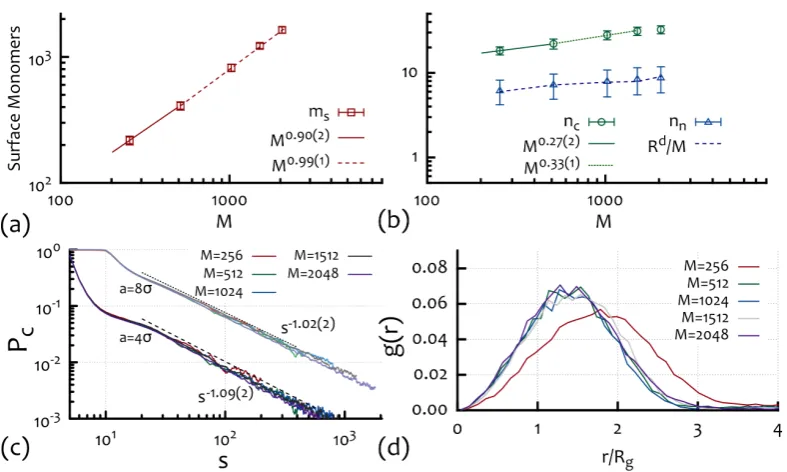
ss−1→ ∞. Numerical [Halverson et al., 2011a,Halverson et al., 2013] and experimental [Lieberman-Aiden et al., 2009,Mirny, 2011] observations in fact report a contact exponent close to, but slightly greater than, unity.

Another useful quantity is how “rough” the coil surface is. This can also be understood in terms of number of contacts nc or inter-blobs§ contacts ng. Let us assign to these two quantities the exponentsβc andβg regulating the scaling of the contacts for ans-monomer long sub-chain as

nc(s)∼sβc (2.21)

being the number of contacts of a given segment with any other segment and

ng(s)∼sβg (2.22)

being the number of contacts between blobs sitting near one another in space. The surface exponentsβcand βg have to be related to one another by the fact that only a numberr(s)d/sof blobs can be neighbours to a given blob, and therefore:

sβc _∼ r(s)

d

s s

βg ₌_sνd−1_sβg _(2.23)

which gives

βc=βg+νd−1 (2.24)

or in the case of a globule (ν = 1/d):

βc=βg. (2.25)

On the other hand, the contact exponent γ is itself related to the surface

ex-§

A blob being a polymer segment made of several (g) monomers where 1 g M and

assuming a size described by the scalingR(g)∼gν withν= 3/5, being not interacting with other

(25)

ponent βc as the number of contacts of a given monomer with other monomers is

P∞

s0_>sPc(r), which gives the total number of contacts of ans-monomer long segment as

sβc _∼_s

∞

X

s0₌_s

s0−γ

∼s−γ+2 (2.26)

or

βc+γ= 2. (2.27)

It is worth stressing that eq. (2.24) and eq. (2.27) are general relations which hold for any fractal structure and do not rely on the fractal globule assumption. Also, from eqs. (2.24) and (2.27) one can infer some restrictions for the values of these exponents, in particular βc ≥ βg and 1 ≤ γ ≤ 1 + 1/d¶. It is also worth noting that for Hilbert curves in 3D for which R ∼ M1/3 (being space filling), the contact surface scales with β = βc = βg = 2/3 which implies γ = 4/3, while, by contrast, the numerical estimation of β for the fractal globule case (see Ch. 4 and [Halverson et al., 2011a]) seems to be close to unity,β '0.95−0.98, implying

γ = 1.02−1.05 compatible with the results from Hi-C contact maps [ Lieberman-Aiden et al., 2009,Zhang et al., 2012] and the findings reported in Ch. 4.

2.1.3 The Structure Factor

Another observable that is worth investigating in order to probe the internal fractal structure of polymer coils is the single-chain static structure factor, S1(q).

Ex-perimentally, this quantity can be measured via light or neutron scattering (refer to [Rubinstein and Colby, 2003] for experimental realisation details). This is defined as

S1(q) =

* 1

M

X

i M

X

j

eiq(ri−rj) +

(2.28)

where the average is taken over polymers, monomer positionsriand over orientations of the scattering wave-vectorq (when the system is isotropic). For wave-vectors|q|

much smaller thanR−_g1 (or length-scales |q|−1 _{much larger than} _R

g), the scattering function gives

S1(q)'M, (2.29)

since all monomers within the coil contribute to the sum. When 2πR−_g1 < q <

2πσ−1, one finds that all monomers nq within the volume q−3 contribute toS1(q).

In this case, the static structure factor relates to the fractal dimension of the chain as

S1(q)'nq'

1

qd_σd

1/νd

= (qσ)−1/ν = (qσ)−dF_. _(2.30)

¶

(26)

In the case of linear polymers in melt the structure factor correctly returns dF = 2 for the whole range 2πR−_g1 < q <2πσ−1 [Kremer and Grest, 1990]. In the case of ring polymers in dense solutions the scaling of eq. (2.28) is less unambiguous and it has been conjectured [Halverson et al., 2011a] that it displays signatures of more complex internal arrangement of the coils (see also Ch. 4).

2.2 Dynamics

2.2.1 Diffusion Coefficient and Relaxation Time

The first theories describing how ring polymers diffuse through either other chains or a gel have been advanced separately by Cates, Rubinstein and Klein [Cates and Deutsch, 1986,Rubinstein, 1986,Klein, 1986]. They share the same spirit, i.e. de-scribing the diffusion of rings in the melt assuming that rings can move in an amoebae fashion through the surrounding (static) obstacles by successive protrusions medi-ated by kink-gas diffusion along the polymer contour [de Gennes, 1979]. Within this framework, “kinks” or “defects” (or excess of mass along the chain) can dif-fuse independently along the polymer contour until they stop their diffusion on a segment of the randomly branched ring structure and contribute to the extension of that segment. By assuming that the kinks perform a 1D random walk along the contour, the time required to span a distanceRg corresponds to the Rouse time and is computed as

τRouse∼M2. (2.31)

The ring can therefore renew its configuration by consecutive kinks diffusion. For a ring made byM segments this takes a time

τ ∼M τRouse =M3 (2.32)

or, equivalently, a diffusion coefficient

DCM ∼

R2_g τ =M

2ν−3_. _(2.33)

Using the field-theoretic exponent in eq. (2.9),i.e. ν= 5/(2d+4), one finally obtains

DCM ∼M−(3d+1)/(d+2), (2.34) which, in 3D, gives DCM ∼M−2 roughly compatible with numerical evidence (see Ch. 4, Appendix B and [Cates and Deutsch, 1986,Halverson et al., 2011b]). Inci-dentally, this result is the same for linear polymers in melt, since the overall size of isolated self-avoiding rings in a background of obstacles (or gels) is described by

(27)

give DCM ∼ M−7/3 which is weaker than the experimentally and computationally observed scaling.

More recently, Milner, Iyer and then Grosberg [Iyer and Arya, 2012,Smrek and Grosberg, 2015] advanced several other theories for the diffusion of a ring polymers among other chains, or “fixed obstacles”. Milner and Newhall [Milner and Newhall, 2010] proposed an approach based on the “centrality” of a node in the lattice animal representation of the ring defined as

ζk= min (M1(k), M−M1(k)) (2.35)

where M1(k) is the size of one of the two sub-trees generated by cutting the k-th

bond of the tree-representation (see Fig. 2.1). They proposed that, analogously to the reptation mechanism in linear polymers, rings undergo diffusion by vacating bonds via the “evaporation” of one of the two sub-trees across that bond. This means that if the centrality ζk of bond k is small, one expects its relaxation to be quick. On the other hand, bonds whose removal produce two sub-trees with similar sizes are expected to take the longest to disappear. Kramers theorem can be used to show that the probability distribution of the nodes’ centrality P(ζ) is given by the weights in Kramers theorem in eq. (2.10) [Rubinstein and Colby, 2003], appropriately normalised:

P(ζ) = PZζZM−ζ

ζZζZM−ζ

'

s

nv−1 8π(nv−2)

M ζ(M−ζ)

3/2

, (2.36)

where nv is the valence of the nodes. This distribution has the feature that most of the nodes have low centrality and therefore relax quickly. One can then proceed by assuming that rings must arrange themselves in order to satisfy such a centrality distribution, and therefore this acts as an effective entropic potential for the rings biasing the mass diffusion as

βUζ =−logP(ζ). (2.37) By performing Monte-Carlo simulations of trees diffusing on Bethe lattices, Milner and Newhall finally concluded that the mass accumulated withinigenerations from a given high-centrality bond scaled as M(i) ∼ ia = i1.5−1.7 and, as a consequence, the variance of the centrality should scale as the mass diffused in a time τζ∼t2 or

h∆ζ2i ∼ta/2 =t0.75−0.85, (2.38)

which leads to a total relaxation time for a tree formed byM nodes, corresponding to the time required for the centrality to diffuse a “distance” of order M, of

(28)

Their result is again roughly compatible with recent findings [Kapnistos et al., 2008, Halverson et al., 2011b], although completely neglects the motion of other chains and, in particular, inter-chain interactions which can explain the even more recent findings [Pasquino et al., 2013,Gooßen et al., 2014,Doi et al., 2015] (see also to Ch. 4).

Smrek and Grosberg [Smrek and Grosberg, 2015] based on the novel description of a ring as an annealed tree made of crumpled branches decorating a self-avoiding path on a Cayley tree, i.e. R ∼ σM1/3 and R ∼ σ2/5L3/5 with L ∼ σM5/9 (or

ν = 1/3,ρ= 5/9 andν/ρ= 3/5), advanced an alternative picture for the dynamics of rings in the melt. By assuming the existence of an “entanglement length” Me below which the chain is Gaussian,i.e. Rblob∼σMe1/2, which is taken as the “blob size”, the Rouse time for a blob can be written as

τblob ∼

ζeMe2σ2

kBT

(2.40)

whereζe is the effective friction of a blob. The chain is formed by g=M/Me blobs and every time a blob moves by Rblob a fraction 1/g of mass contributes to the

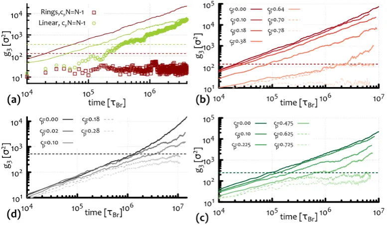
overall diffusion of the centre of mass. The displacement of the chain center of mass, defined as

hδr_CM2 i ≡g3(t) =

D

[rCM(t+t0)−rCM(t0)]2

E

t0

(2.41) where h. . .i_t₀ indicates average over different initial time-steps, can therefore be written as the displacement ofgρblobs of size Rblob forming the backbone L:

hδr_CM2 i ≡g3 'gρ

σMe1/2

g

!2

=Megρ−2σ2 (2.42)

that gives a diffusion coefficient of the blobs along the backbone ofDbb∼g3/τblob.

The full relaxation of the chain can be achieved once the centre of mass has travelled the ring’s size L,i.e.

τrelax∼

L2 Dbb

=τblobgρ+2 (2.43)

where one uses the fact thatL∼Me1/2gρσ giving

τrelax∼

ζeσ2

kBT

M23/9. (2.44)

The diffusion coefficient of the whole ring can be found by imposing that the ring is displaced a distance equal to its own size (R =σMe1/2gν) in the relaxation time

τrelax,i.e.

DCM ≡

R2

τrelax

∼ Meσ

2

τblob

g2ν−ρ−2'DblobM−17/9. (2.45)

(29)

ev-2. Predicting the Behaviour of Rings in Solution 19

idence, although they predict exponents that underestimate the observed ones. In particular, none of these explain why the sub-diffusion of the rings can be observed on length-scales many times the ring’s gyration radius [Halverson et al., 2011b, Halver-son et al., 2014]. This may be due to chains moving and interacting non-trivially with one-another. The main reason for this is that mean-field theories analyse the behaviour of chains among other “fixed” chains. This is not the case in ring polymer melts where inter-chain interactions are important (see Ch. 4 and [Halverson et al., 2011a]) and lead to collective behaviour. In order to correctly capture the dynamics of rings in the melt one should take into account the collective re-arrangements and configurational fluctuations, which makes the problem much harder to tackle.

2.2.2 How Rings Relax Stress

How rings relax their stress is perhaps one the key questions that I will try address. Recently there have been quite a few attempts to quantify the stress relaxation of rings in a background of obstacles [Milner and Newhall, 2010] and in the melt [ Kap-nistos et al., 2008,Pasquino et al., 2013,Smrek and Grosberg, 2015]. All the the-oretical effort has been focused on describing rings as amoebae [Rubinstein, 1986] moving through obstacles situated around the ring double-folded configuration, i.e. not threading its contour. This strong assumption seems now ubiquitous when tack-ling the ring melt problem. On the contrary, I will show for the first time that this is instead not a correct assumption: Rings do protrude through one-another, and this has strong consequences on the dynamics, which should be considered when formulating a theory of their stress relaxation (see Ch. 4).

Experimentally there is several evidence that melts of rings display a very low stress-relaxation modulus G(t) which never exhibits a plateau [Kapnistos et al., 2008,Pasquino et al., 2013]. One the other hand, their slow overall relaxation to free diffusion [Halverson et al., 2011b] as well as a dramatic viscosity enhancement observed in more recent findings [Doi et al., 2015] indicate that inter-coil interactions are important but hard to quantify.

(30)

While the internal relaxation of linear polymers is intimately related to the per-sistence of their neighbours forming the surrounding tube, this cannot be said for ring polymers, which can create new protrusion anywhere along their contour, being not limited by the presence of fixed ends. On the other hand, threadings, which are only possible between ring polymers, might affect the overall relaxation,i.e. the diffusion of the centre of mass of the polymers, leaving the internal stress relaxation mechanisms unaffected. In light of this I propose to focus on measuring the long-time inter-coil correlations which can be most readily done via scattering methods, and in particular via the coherent scattering functionSc(q, t), defined below.

2.2.3 Inter-Coil Correlations Probed by Dynamic Scattering

Intra-coil correlations on length-scales l= 2πq−1 are commonly probed by the co-herent (or in-coco-herent) dynamic scattering function Sc(q, t) (or Sin(q, t) obtained setting i=j):

Sc(q, t) =

* 1

M

X

i M

X

j

eiq(ri(t+t0)−rj(t0))

+

, (2.46)

where the average is taken over the rings in the system and differentt0. In practice,

one can imagine one probe chain in the solution scattering the incident light and then repeating the measurement over many different probe chains. This function is also sometimes called the “self-intermediate scattering function” and its Fourier transform the “self-part of the Van Hove function” in the glass-transition commu-nity [Berthier and Biroli, 2011], where it is one of the main tools used to capture density-density correlations in a glass-forming systems. This scattering function was also studied by de Gennes [de Gennes, 1981] to capture the behaviour of one reptating linear chain among other fixed chains.

In some cases, especially when dealing with molecular liquids or liquids made of simple constituents, the dynamic scattering function can give some information re-garding inter-objects correlations, being internal degrees of freedom not included in the picture. In the case of polymer liquids, characterising inter-coil correlations via the dynamic scattering function can be less straightforward [Aichele and Baschnagel, 2001,Frey et al., 2015]. In particular, it is sometimes necessary to extend the compu-tation of eq. (2.46) to all the atoms in the system, rather than the ones forming the chainsk. In this case the function is also known as the (dynamic) “pair-correlation” function, which is rarely studied as numerically infeasible to compute throughout the simulation.

In light of this one is often limited to the computation of eq. (2.46) over the beads forming a single chain and to take the average over many chains. This means that

Sc(q, t) formally captures intra-coil correlations, and does not give direct evidence

k

In this case the computation can scale as (N M)2_{, for a system of}_N _chains _M _{beads long,}

(31)

of inter-coil correlations. On the other hand, it is possible to infer some information on the inter-coil correlations whenq becomes greater than the inter-coil distance 2λ, whereλis defined as

λ=φ−1/3Rg (2.47)

whereφ is the coils volume concentration,i.e.

φ= 4N πR

3

g

3σ3_L3 . (2.48)

The free volume available to the coils is 1/φ and hence the free length (in units of the radius of gyration of the polymers) is φ−1/3. This means that above overlap the inter-coil distance is smaller than 2Rg.

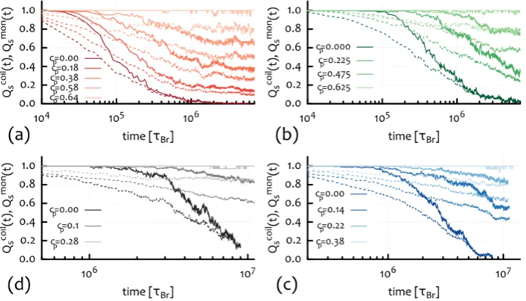
The information that one can obtain from Sc(q, t) on the collective behaviour of the rings is based on the following reasoning: the dominant contribution toSc(q, t) comes from beadsjthat have not travelled (much) further than 2π/qfrom the other bead i within t time-steps. Therefore if there was a length-scale above which the independent motion of the beads was somehow constrained, that would appear when probing the system with the right q. In particular, one can imagine that if a ring was permanently pinned down by a frozen obstacle threading through its contour then one should expect

lim

t→∞Sc(q 'πR −1

g , t) =Sc∞(q'πR−g1)>0 (2.49) where S_c∞(q) is a constant greater than zero and near one, as most of the beads forming the chain would be forever trapped in a region of linear size l '2Rg. On the other hand, if one was to probe larger q’s,i.e. shorter length scales, one should in principle observe a more unconstrained relaxation, and in particular

lim

t→∞Sc(q &πR −1

g , t)'0. (2.50)

Although it is worth bearing in mind that this scattering function would not decay strictly to zero, as presence of permanent obstacles, i.e. regions that the beads are not free to explore, has the effect of suppressing the full de-correlation of the monomers.

(32)

2πq−1 &2Rg) compared to a ring that is instead not threaded. Both, threaded and non-threaded rings, should instead relax their internal (i.e. 2πq−1 .2Rg) stress at roughly the same rate,i.e. having the same decay ofSc(q&πR−g1, t).

(33)

It is nice to know that the

computer understands the problem . . . But I would like to understand it too.

E. Wigner

3

Molecular Dynamics Models

Contents

3.1 Molecular Dynamics Scheme . . . 24

3.1.1 Non-Bonded Potentials . . . 25 3.1.2 Bonded Potentials . . . 26 3.1.3 Brownian Dynamics . . . 27

3.2 Modelling . . . 30

3.2.1 Modelling (Knotted) Ring Polymers . . . 31 3.2.2 Modelling a Physical Gel . . . 35

C

omputersimulations, or “experiments” [Frenkel and Smit, 2001], are

im-portant tools for studying complex systems. This Thesis itself largely relies on computational methods, in particular Molecular Dynamics (MD) sim-ulations. For this reason, I devote this chapter to describing the essence of the MD simulations employed here and the computational details of the models described in the subsequent Chapters.

Molecular Dynamics simulations have been used for the first time in the late 50’s [Alder and Wainwright, 1959]. They started as a method to investigate the properties of systems of hard spheres [Alder and Wainwright, 1957] and simple liquids [Rahman, 1964] and later became a fundamental technique to model the dynamics of biomolecules [McCammon et al., 1977,Karplus and Petsko, 1990]. As opposed to standard Monte-Carlo techniques, MD simulations offer the advantage of naturally probing the dynamical properties of the systems, such as transport coeffi-cients, time-dependent responses and rheological properties. In addition, Molecular Dynamics models are very flexible in terms of the level of coarse-graining performed on the model. They can either be very accurate in describing microscopic molecular details or in evolving a more coarse-grained picture, depending on the level of detail needed. Usually, MD models lend themselves to a much higher level of molecular

(34)

3. Molecular Dynamics Models 24

detail, than standard Monte-Carlo models. One of the key challenges of MD mod-els is to include the appropriate inter-molecular potentials, and, in particular, find the right level of coarse-graining required to reach the best accuracy given practical constraints on their feasibility.

Because modelling microscopic chemical interactions are computationally expen-sive and much of the puzzling physical features of rings in solution are hidden in their long-time behaviour, my interest is in retaining only the key physical elements. I therefore adopt coarse-grained models for the polymers in order to reach longer simulations time-scales. In particular, I will formulate a mesoscopic physical model of the polymers and neglect specific chemical details. Some of the problems dis-cussed in the following Chapters will be naturally associated with specific types of polymers. For instance, gel electrophoresis is very often performed on DNA sam-ples, and therefore it is natural to start from a more physically faithful description for the DNA. On the other hand, the chemical details of the base-pair system is not necessary to capture the physics of gel electrophoresis and will, therefore, be coarse-grained out. In addition, addressing more coarse-grained models has often the advantage of delivering more general results, which might be valid for other systems, as long as they share similar physical and topological properties.

In what follows, I will firstly discuss some general elements of Molecular Dynam-ics simulations and secondly, I will give describe in detail the coarse-grained models used in the following Chapters.

3.1 Molecular Dynamics Scheme

The aim of a Molecular Dynamics simulation is to integrate the classical equations of motion:

∂ri

∂t =vi mi

∂vi

∂t =Fi =− ∂U

∂r, (3.1)

(35)

3.1.1 Non-Bonded Potentials

Each atom in the simulation can interact via non-bonded potentials with all the other atoms in the system and, if present, a wall delimiting the simulation box. Because of this, one needs to define the 1-body, 2-body, 3-body, etc. interactions as

Unb = N

X

i

u(ri) +

X

i

X

j>i

v(ri,rj) +. . . (3.2)

where u(ri) is the potential describing the interaction between a single atom and, for instance, a wall andv(ri,rj) the potential describing a 2-body interaction,e.g. a Lennard-Jones or Coulomb potential. For instance in the case of charged polymers, one should, in principle, include both steric and Coulomb interactions. It is also common, as long as the simulation reproduces the essential physics, to drop all the higher order terms.

The two-body repulsion can be efficiently modelled via the following shifted-truncated form of the Lennard-Jones (LJ) potential (or Weeks-Chandler-Andersen model [Weeks et al., 1971]):

U_LJ(ri,rj) = 4

" σc rij 12 − σc rij 6 + 1 4 #

Θ(21/6σc−rij), (3.3)

where Θ(x) is the usual Heaviside function,i.e. 1 forx≥0 and 0 otherwise, and σc is the minimum distance between beads. The potential depth isand rij =|ri−rj| is the distance between the i-th and j-th atom. This version of the Lennard-Jones potential is chosen in order to broadly model only the steric repulsion between atoms, thereby avoiding (i) unwanted Van der Walls attractions and (ii) long-ranged interactions without introducing discontinuity in the potentials.

Another useful way of modelling steric interactions is via a “soft” potential. One of the most used forms of this potential is the following:

U_soft(ri,rj) =s

1 + cos

πrij

rc

Θ(rc−r). (3.4)

(36)

3.1.2 Bonded Potentials

Bonded potentials describe the interactions between atoms which share molecular bonds. The simplest potential describing the connection between two atoms is the harmonic potential that models the bond as a spring with stiffness κh and equilib-rium lengthr0:

U_harm(ri,rj) =

κh

2 [rij−r0]

2

. (3.5)

This potential is usually inappropriate for use in polymer chains simulations, espe-cially in dense conditions, as it can allow bonds to stretch and polymers to cross through one-other. More appropriate 2-body bonded potentials exist for system of polymers, such as the Finitely Extensible Non-linear Elastic (FENE) potential:

UFENE(ri,rj) =−

κf 2 R

2

0ln

" 1−

rij

R0

2#

, (3.6)

for rij < R0 and UFENE(ri,rj) = ∞, otherwise. The values of the parameters chosen here in this Thesis are R0 = 1.6 σ and κf = 30 /σ2. These choices ensure that strand-crossing events are suppressed. This is of paramount importance when the topological state of a polymer, e.g. (un-)knotted or (un-)linked, needs to be preserved throughout the simulation.

In order to model the chains stiffness, the following 3-body bonded potential is commonly used:

U_bend(ri,rj,rk) =

kBT lp

σ

1−rij ·rjk

rijrjk

= kBT lp

σ [1−cosθ], (3.7)

where the angle θ is defined as the angle between consecutive bonds (see Fig. 3.1). Here,rij ≡rj−riis the vector joining two bonded monomers andlpis the persistence length which corresponds to half the Kuhn length lK [Doi and Edwards, 1988]. For instance, to correctly model hydrated double-stranded DNA (dsDNA) chain embedded in a solvent in physiological conditions, one should take its persistence length to belp =lK/2'20σ,i.e. roughly 20 times its thickness.

A 4-body bonded interaction can be used to capture the torsional stiffness of polymers: The most common choice in this case is a dihedral potential, which can be modelled as a CHARMM [MacKerell et al., 1998] potential:

Udihedral(ri,rj,rk,rl) =κd[1 + cos (nφ−d)] (3.8)

where κd is the spring energy, n ≥ 0 is a free parameter, d an integer number of degrees and φ is defined as the angle between the planes defined by the triplets of atoms ijk and jkl (Fig. 3.1). The angle φ is defined as cosφ = nˆijk·nˆjkl where

(37)

Figure 3.1: The angle θ for the bending potential in eq. (3.7) is defined as the angle between the vectors joining consecutive pairs along the polymer contour. The angle φfor the dihedral potential in eq. (3.8) is defined as the angle between the planes defined by the pairs of vectors rij,rjk and rjk,rkl connecting the polymer backbone (greybeads) to the

patches to the sides (blue orred).

consequent supercoiling properties [Brackley et al., 2014].

3.1.3 Brownian Dynamics

When the subject of the “computer experiment” involves a solvent, and the hydro-dynamic interactions can safely be neglected, it is common practice to model the solvent “implicitly”. Instead of integrating the deterministic motion of the small solvent particles, one can couple the beads forming the solute with a bath at fixed temperatureT: this implies that every atom in the system undergoes some motion which is no longer deterministic but includes a stochastic term. This is modelled as a force that represents the random (frequent) collision of the solute with the sol-vent (much smaller) particles. This method of simulating systems where the solute molecules are much heavier than the solvent ones is often referred to as “Brown-ian Dynamics”. The equation describing the motion of the atoms is the Langevin equation:

mi

∂2ri

∂t2 =−ξi

∂ri

∂t − ∂U

∂r + p

2kBT ξifi (3.9) wherefi is a delta correlated white noise with zero mean

D

f_iα(t)f_jβ(s) E

=δ(t−s)δijδαβ (3.10) along each Cartesian component (Greek letters) and ξi is the friction coefficient of the i-th atom. In the limit in which the term on the left hand side of eq. (3.9) is neglected, i.e. in the long-time limit t mi/ξi, the Langevin equation takes the “over-damped” form:

∂ri

∂t =−

1

ξi

∂U

∂ri

+p2Difi (3.11)