http://wrap.warwick.ac.uk
Original citation:
Aldegunde, Manuel, Kermode, James R. and Zabaras, Nicholas. (2016) Development of
an exchange–correlation functional with uncertainty quantification capabilities for density
functional theory. Journal of Computational Physics, 311 . pp. 173-195.
Permanent WRAP url:
http://wrap.warwick.ac.uk/77127
Copyright and reuse:
The Warwick Research Archive Portal (WRAP) makes this work by researchers of the
University of Warwick available open access under the following conditions. Copyright ©
and all moral rights to the version of the paper presented here belong to the individual
author(s) and/or other copyright owners. To the extent reasonable and practicable the
material made available in WRAP has been checked for eligibility before being made
available.
Copies of full items can be used for personal research or study, educational, or
not-for-profit purposes without prior permission or charge. Provided that the authors, title and
full bibliographic details are credited, a hyperlink and/or URL is given for the original
metadata page and the content is not changed in any way.
Publisher’s statement:
© 2016, Elsevier. Licensed under the Creative Commons
Attribution-NonCommercial-NoDerivatives 4.0 International
http://creativecommons.org/licenses/by-nc-nd/4.0/
A note on versions:
The version presented here may differ from the published version or, version of record, if
you wish to cite this item you are advised to consult the publisher’s version. Please see
the ‘permanent WRAP url’ above for details on accessing the published version and note
that access may require a subscription.
Development of an Exchange-Correlation Functional with Uncertainty
Quantification Capabilities for Density Functional Theory
Manuel Aldegunde, James R. Kermode, Nicholas Zabaras∗
Warwick Centre for Predictive Modelling, University of Warwick Coventry CV4 7AL, United Kingdom
Abstract
This paper presents the development of a new exchange-correlation functional from the point of view of machine learning. Using atomization energies of solids and small molecules, we train a linear model for the exchange en-hancement factor using a Bayesian approach which allows for the quantification of uncertainties in the predictions. A relevance vector machine is used to automatically select the most relevant terms of the model. We then test this model on atomization energies and also on bulk properties. The average model provides a mean absolute error of only 0.116 eV for the test points of the G2/97 set but a larger 0.314 eV for the test solids. In terms of bulk properties, the prediction for transition metals and monovalent semiconductors has a very low test error. However, as expected, predictions for types of materials not represented in the training set such as ionic solids show much larger errors.
Keywords: Bayesian, Density Functional Theory, Exchange-Correlation Functional, Uncertainty Quantification
PACS:71.15.Mb, 71.15.Nc, 31.15.eg
2010 MSC: 62F15, 82-04
1. Introduction
In the last several decades, density-functional theory (DFT) has become the most widespread framework to study materials from a fully quantum-mechanical perspective due to the favorable trade-offbetween accuracy and computa-tional cost it provides. Even though the theory in principle is exact, its application calls for the use of approximations, some because of computational reasons, such as the Born-Oppenheimer approximation, and some because the exact term is not known, as is the case with the exchange-correlation (XC) energy. Even though the accuracy of the different approximations has been tested in many fields, the error that they lead to when DFT is applied to new systems remains a concern, which limits the predictive power for new systems.
Recently, several works have been published which try to address this problem from different points of view. K. W. Jacobsenet al.have applied the concepts ofsloppy models[1] to DFT [2, 3, 4, 5, 6]. These are models in which a part of the model parameters, thesloppy parameters, are largely unimportant for the model predictions, so that they can only be determined with large uncertainty. In this framework, they start with a modelMwhich depends on a set of parameters,θ. To find the probability of a given parameter set,θ, given the model,M, and a database of experimental data,D, a Boltzmann distribution is assumed for a cost functionC(θ), which can be, for example, a least squares cost function with [2] or without [4, 6] regularisation:
P(θ| M,D)∼exp(−C(θ)/T), (1)
whereTis an “effective temperature” which determines the spread of the ensemble and therefore the error estimation. This distribution of the parametersθis then used to generate ensembles of XC enhancement factors that can be used
∗
Corresponding author
Email addresses:[email protected](Manuel Aldegunde),[email protected](James R. Kermode),[email protected](Nicholas Zabaras)
to estimate errors in different quantities. This model was used to train a meta-generalized gradient approximation (meta-GGA) exchange-correlation functional, mBEEF, using experimental data for bulk solids (lattice constant and cohesive energies), molecules (formation energies and molecular reaction energies) and surfaces (chemisorption on solid surfaces) [4, 6].
Also recently, K. Lejaeghereet al.have studied errors in DFT simulations from a different perspective [7]. Instead of trying to construct a new functional, they analyse the errors for a give XC functional in terms of a linear regression model between experimental and calculated data. The least-squares estimate of the slopeβis taken as a measure of systematic errors, and the errorεgives the residual error bar. The scatter in DFT results comes from the ability of the XC functional to represent some materials better than others. They carry out this study on the ground-state elemental crystals at 0 K up to Rn. In this case, the prediction of the properties for a new compound not included in the set is done by applying the correction for systematic deviation and adding the residual error,xpred =βxDFT±ε,
wherexpredis the corrected prediction for the magnitudex,βrepresents the systematic deviation,xDFTthe magnitude
obtained from the DFT simulation andεthe residual error which models the inability of the DFT model to reproduce the experiment exactly.
In this work, we present the development of a new meta-GGA exchange-correlation functional with uncertainty quantification capabilities from the point of view of machine learning extending on the work of Wellendorffet al.[6]. We use a Bayesian approach for the determination of the regression coefficients with a relevance vector machine. Unlike the sloppy model approach using regularised least squares in [6], the use of a relevance vector machine auto-matically selects the most relevant terms and drops the rest, which avoids the possibly very large number of terms in the linear model and helps avoid overfitting.
In Section 2, we present the basics of DFT and the formulation of a linear model for the exchange energy func-tional. Next, in Section 3, we detail the Bayesian linear regression framework used to obtain the coefficients of the model as random variables. We also discuss how from these parameters we can get a predictive distribution for the modelled function and also the use of a relevance vector machine to allow for automatic model determination. The actual training of the model using atomization energies is presented in Section 4, which describes in more detail how to set up all necessary data from DFT simulations. We also include a description of how it is possible to use some indirect measurements to extend the available data set for training as well as a description of the training set we used. Numerical results testing the proposed framework are presented in Section 5 for atomization energies of molecules and solids. Even though the training data consists of energies, we can also use the framework to propagate uncer-tainties to other derived quantities such as bulk properties. Section 6 describes an example of this process using an equation of state, which inserts an extra layer of uncertainty. Then, numerical examples of propagation of uncertainty are shown for two bulk properties of solids, equilibrium lattice constants and bulk moduli, and for the band gap of Si. Finally, we end up summarizing the main contributions of this work as well as the numerical results and how they compare to other available XC functionals.
2. Density Functional Theory
DFT approximates the ground state energy of a material system with charge density n [8, 9]. It does so by minimizing the energy functionalEDFT[n] for a given system. This functional is given by [10]:
EDFT[n]=
Z
n(r)v(r)dr+T0[n]+U[n]+Exc[n]
=Eb[n]+Exc[n]=Eb[n]+Ex[n]+Ec[n], (2)
whereris the position in real space,v(r) is an external potential,T0[n] is the non-interacting kinetic energy,U[n] the classical electron-electron repulsion energy andExc[n] is the XC energy functional, which is not known exactly.Eb[n]
groups all the contributions not coming from exchange and correlation. Exc[n] has two components, the exchange
energyEx[n] and the correlation energyEc[n] [10].
the Schr¨odinger equation for non-interacting particles [9]:
"
−1
2∇
2+v
e f f(r) #
ψi(r)=iψi(r), (3)
where−1 2∇
2is the kinetic energy operator,ψ
i(r) are the Kohn-Sham orbitals,iare the Kohn-Sham orbital energies
andve f f(r) is an effective potential composed by the external potential, the electron-electron interaction and the XC
potential [9, 10]:
ve f f(r)=v(r)+
Z n(r0) |r−r0|dr
0+
vxc(r). (4)
The XC correlation potential is related to the XC energy through a functional derivative with respect to the density,
vxc(r)=δE
xc[n]
δn(r) [9]. The Kohn-Sham orbitals can be used to obtain the electron density of the system [9],
n(r)=X
i
|ψi(r)|2. (5)
Since the effective potential is itself a functional of the density, Eqs. (3)-(5) need to be solved self-consistently, i.e., they have to be iterated until convergence.
2.1. Exchange-Correlation energy
Even though this formulation of the problem is favorable for numerical computation, there still remains the ques-tion of approximating the XC energy and potential since, as we noted before, it is unknown in general.
In [12], J. P. Perdewet al. introduced a hierarchy of approximations called “Jacob’s ladder”. If we write the XC energy as
Exc[n]=
Z
nεxc(n;r)dr, (6)
where the productnεxcis an XC energy density andεxcis an XC energy per electron, we can see the ladder as
increas-ingly complex approximations forεxc. At the lowest level, the local density approximation (LDA),εxc depends only
onn(r), the density at the position where the energy is evaluated. A second level includes as well the density gradient,
∇n(r), and it is called the generalized gradient approximation (GGA). Since it also includes derivative information this type of approximation is called semi-local. Two of the most widely used GGA functionals are the Perdew-Burke-Ernzerhof (PBE) functional [13] and a revision to improve results for solids which modifies two of its parameters, PBEsol [14]. The third level of the hierarchy is the meta-generalized gradient approximation (meta-GGA), which adds dependence on the Kohn-Sham orbitals. Since the Kohn-Sham orbitals are in general non-local functionals of the electron density, meta-GGA approximations are also non-local. However, since meta-GGA functionals are con-structed to be local in the orbitals, which are readily available from the solution of the eigenvalue problem, they retain much of the computational efficiency of the GGA [12]. Popular functionals in this category include the Tao-Perdew-Staroverov-Scuseria (TPSS) functional [15], mBEEF [6], or the “Made Simple” (MS0) functional [16]. Higher levels of the hierarchy include ingredients such as the exact expression for the exchange energy,
Ex[n]=−1
2
X
i Z ψ∗
i(r)ψi(r0)
|r−r0| drdr
0. (7)
Hybrid functionals, which combine this exact exchange with semi-local functionals are especially popular in chem-istry, and some of the most widely used are the Becke-3-Lee-Yang-Parr (B3LYP) [17], PBE0 [18] and M06 [19].
Because of the non-locality of this last family of functionals, the computations are much more demanding, so in this work we restrict ourselves to the meta-GGA approximation.
2.2. Exchange energy in meta-GGA
At the meta-GGA level of approximation, the XC functional can be written as [20]
Exc[n]=
Z
whereτ(r)=2P0 i
1 2|∇ψi(r)|
2
is the kinetic energy density. The summationP0
iruns only over the occupied Kohn-Sham
orbitalsψi(r).
To specify the exchange energy contribution, it is common to introduce theexchange enhancement factor,Fx(n,∇n, τ),
which contains all the contributions to nonlocality through its dependence on the gradient of the electron density∇n
and the kinetic energy densityτ. Using it, the exchange energy functional can be written as [20, 21, 22]
Ex[n]=
Z
nεx(n,∇n, τ)dr=
Z
nεU EGx (n)Fx(n,∇n, τ)dr, (9)
whereεx(n) is the exchange energy per particle of the system andεx
U EG(n)=−3(3π
2n)1/3/(4π) is the exchange energy
per particle of a uniform electron gas.
Furthermore, the dependence on the density gradient and the kinetic energy density is usually transformed into the dimensionless parameterss, the reduced density gradient, andα, the dimensionless deviation from a single orbital shape [20, 23]:
s= |∇n|
2(3π2)1/3n4/3; α= τ−τW
τU EG , (10)
whereτW=|∇n|/8nandτU EG= 3 10(3π
2)2/3n5/3are the Weizs¨acker and uniform electron gas kinetic energy densities,
respectively. Using these parameters, the exchange energy functional can be written as [22, 24]
Ex[n]=
Z
nεxU EG(n)Fx(s, α)dr. (11)
2.3. Linear model for the exchange energy
To specify a DFT approximation, we have to provide two models for the exchange and correlation functionals,
Ex[n;ξx] andEc[n;ξc], whereξxandξcare two sets of parameters which determine the XC model [10], and can be
determined either empirically, fitting them to experimental data [6], or from theoretical considerations [22]. Putting these parameters explicitly, the DFT energy functional is then
EDFT[n;ξx,ξc]=Eb[n]+Ex[n;ξx]+Ec[n;ξc]. (12)
Following the previous studies in [2, 4], we will focus on the exchange contribution only, taking the correlation energy term from other functionals. In particular, we will compare the use of the correlation terms from the XC functionals PBE, PBEsol, MS0 and TPSS.
To specify our exchange energy model, we will use the exchange enhancement factor, whose functional form is not known [24]. In this work, we follow [4] and represent it as a linear model in a set of basis functionsφi(s, α),
Fx(s, α)=X
i
ξx
iφi(s, α)=(ξx)Tφ(s, α), (13)
where we have introduced a vector notation for the linear model coefficientsξx ={ξx
i}and basis functionsφ(s, α)=
{φi(s, α)}.
Also following [4], we use a truncated Legendre polynomial expansion on rational transformations of the param-eterssandα:
Fx(s, α)=
Ms
X
i Mα
X
j
ξx
i jPi(ts(s))Pj(tα(α)), (14)
wherePi(x) is the Legendre polynomial of order ion x, Ms and Mα are the orders of the expansion for sandα,
respectively, andξx
i jis the enhancement factor linear model coefficient for ordersi, j. The transformations onsandα
are defined as
ts(s)=
2s2
and
tα(α)= (1−α
2)3
1+α3+α6, (16)
where the parameterqin Eq. (15) isq=κ/µGE, withκ=0.804 andµGE =(10/81). These parameters are used in the PBEsol exchange functional [14], which is the basis for this transformation. In fact,ts(s) is the PBEsol enhancement
factor scaled to the interval [−1,1) fors≥0 [6]. On the other hand,tα(α) is theαdependence of the MS0 exchange enhancement factor [16], which is confined to the interval (−1,1] forα≥0.
Using this linear model for the enhancement factor, we can write our model exchange energy as
Ex[n;ξx]=
Z
nεU EGx (n)
M X
i=1 ξx
iφi(s, α)dr
=
M X
i=1 ξx
i Z
nεxU EG(n)φi(s, α)dr= M−1
X
i=0 ξx
iE x
[n;ˆei]=(ξx)TEx[n;ˆe], (17)
whereM = Ms×Mα andEx[n;ˆei] is the exchange energy obtained using the unit vector ˆeias coefficient vector in
Eq. (13), i.e.,φi(s, α) as the enhancement factor. Ex[n;ˆe]={Ex[n;ˆei]}is the vector notation for the exchange energy
functionals obtained this way. From now on, we will drop the superscriptxin the parameters since they will be the only ones we use,ξ≡ξx.
The exchange energy can be seen as a linear model where the basis functions are given by exchange energies with
φi(s, α) as the enhancement factor.
Remark 1. In this work, we will construct a surrogate model for the exchange energy functional, Ex[n], given by Eq. (17), where the coefficients are random variables whose distribution will be determined by the regression process described in Section 3. The randomness of the model will account both for model error and the limited data (epistemic uncertainty) that are used to compute the distribution ofξ.
Remark 2. In the context of DFT, energy and all other quantities of interest are functionals of the electron density. In particular, the exchange-correlation energy is a functional of the electron density. However, the specification of a new system on which we want to make predictions is usually obtained as a configuration of atoms in space. Therefore, to calculate its electron density a self-consistent solution of Eqs. (3)-(5) is required.
This means that in order to make predictions our surrogate model still has the cost of a self-consistent simulation as an electron density is needed to use it. This is unlike a typical regression problem where, given an input, the surrogate model would give a prediction for the output bypassing the need to run the full model and thus having a higher computational efficiency.
Remark 3. From Eq. (17), we can see that to obtain the exchange energy for a system swith electron densityn,
Ex[n;ξx], we need to evaluate each of the exchange functional basis,Ex[n;ˆe
i], for the same value of the density,
n. For the training of the system, one needs to evaluate the basis functionals for the density of the training material systems. We assume here that the change in the charge density obtained performing self-consistent calculations with different XC functionals is small, which is in general a good approximation due to the variational principle [2] and has also been shown numerically [25]. This means that, as long as the density is obtained self-consistently, the XC functional chosen to calculate it is of secondary importance in the evaluation of the basis functions in Eq. (17). Under this assumption to carry out the training of the model, we can obtain the density for every system of interest running a self-consistent simulation with a common functional. If we denote the density of the training systemsasn∗s, we can then calculateEx[n∗s;ˆei] (values of the basis functions in the training charge densities), using the PBE functional as a
common functional, i.e.,n∗s will be the self-consistent density obtained using the PBE XC functional for all training
systemss.
3. Bayesian Linear Regression
instead of point quantities as with, for example, classical least squares regression. The Bayesian model will allow us to quantify the uncertainty in predicted values for unseen material systems, as long as these test systems are relevant to the materials used in the training of the model.
In what follows, we use the following notation for the probability distributions that will arise in the description of the model:
• N(x|µ,S) is a Gaussian distribution onxwith meanµand covarianceS,
• G(x|α, β) is a Gamma distribution onxwith parametersαandβ,
• St(x|µ,Λ, ν) is a Student t-distribution onxwith parametersµ,Λandν.
Formally, the procedure involves assuming that a set of experimental or numerically generated datatare avail-able representing noisy observations ofEx[ni] for various densitiesni. The linear model for the underlying process
generating the data is of the form:
Ex[n;ξ]=
M X
i=1
ξiEx[n;ˆei], (18)
whereξiare the M parameters of the model andEx[n;ˆei] are the basis functions. The first aim of Bayesian linear
regression is to compute aprobability distributionfor the parametersξ={ξi}of the linear model given the observed
data, i.e., p(ξ|t).
Remark 4. In this work, the model parametersξonly appear on the exchange energy term, so that the full model for the energy is
E[n;ξ]=Eb[n]+Ec[n]+
M X
i=1
ξiEx[n;ˆei]. (19)
We have chosen to transform the experimental data subtracting the energy contributionsEb[n] andEc[n] obtained
from simulations. For every training system, we run a self-consistent simulation and subtract these energy terms from the experimentally observed energies. From now on, we will refer to these energies which are obtained using both experimental and simulated data simply as theenergy training data set.
We will assume that the observed datatfollow on average our model exchange functional,ξTEx[n;ˆe], and have an
additional error termε. This quantity represents the model accuracy as it provides a measure of the deviation between our model and the experimental results. Therefore, for a single observationti,
ti=ξTEx[ni;ˆe]+εi, (20)
whereεi is an error term. Under the assumption of Gaussian error with the same precision for all data points,β =
1/v=1/σ2, wherevis the variance andσthe standard deviation, the probability of getting a particular value for the observation for a material system with charge densityniwill follow a Gaussian distribution with meanξTEx[ni;ˆe]:
ti∼ N(t|ξTEx[ni;ˆe], β−1). (21)
The likelihood functionLgives a measure of how likely it is to obtain the observed datatgiven the assumed model. In our case it will be
L(t|n,ξ, β)=
N Y
i=1
N(ti|ξTEx[ni;ˆe], β−1), (22)
whereNis the number of experimental data,n={ni}are the densities of the input system,ξare the coefficients of the
linear model andβis the noise precision.
• Prior onξ: p(ξ|β,m0,S0)=N(ξ|m0, β−1S0)
• Prior onβ: p(β|a0,b0)=G(β|a0,b0)
m0,S0,a0andb0are parameters which define the distribution over the model parameters and are called
hyperparam-eters [26]. Section 3.2 will explain how they are determined from the data.
With the chosen priors for each model parameter, the joint prior probability distribution over our model parameters becomes
p(ξ, β)=p(ξ|β)p(β)=N(ξ|m0, β−1S0)G(β|a0,b0). (23)
Given the likelihood and the prior, we can obtain the posterior probability distribution of the parameters given the data using Bayes’ theorem [26]:
p(ξ, β|t)=R L(t|n,ξ,β)p(ξ, β)
L(t|n,ξ,β)p(ξ, β)dξdβ =N(ξ|mN, β −1S
N)G(β|aN,bN). (24)
Details on how to arrive at Eq. (24) can be found in Appendix A. The parameters of the posterior distribution are:
S−N1=S−01+ΦTΦ, (25)
mN =SN h
S−01m0+ΦTt
i
, (26)
aN =a0+N/2, (27)
bN =b0+
1 2
mT0S−01m0−mTNS
−1
N mN+tTt
. (28)
Finally, we have introduced thedesign matrixΦdefined as:
Φ=
Ex[n∗1;ˆe0] · · · Ex[n∗1;ˆeM−1] Ex[n∗2;ˆe0] · · · Ex[n∗2;ˆeM−1]
..
. ... ...
Ex[n∗
N;ˆe0] · · · E x[n∗
N;ˆeM−1]
=
Ex[n∗ 1;ˆe]
T
Ex[n∗ 2;ˆe]
T
.. . Ex[n∗
N;ˆe] T , (29)
wheren∗
i,i=1. . .Nare the self-consistent densities using the PBE XC functional for each of theNmaterial systems
used in the training set of our linear regression problem.
Remark 5. Further theoretical constraints on the XC energy such as the Lieb-Oxford bound [10], which gives a theoretical upper bound for the exchange enhancement factor, can be imposed through the prior, even though the resulting posterior would require numerical methods such as Markov Chain Monte Carlo for sampling.
3.1. Predictive distribution
Once we have a distribution for the model parameters, we can calculate the probability distribution of the output of our model, ˜t, given an input system with density ˜n. This is called thepredictive distributionand it is computed by averaging the likelihood of ˜tgiven ˜nover all sets of the parameters defined by the posteriorp(ξ, β|t),
p(˜t|n˜,t)=
Z
p(˜t|n˜,ξ, β)p(ξ, β|t)dξdβ
=Z N(˜t|ξTEx[˜n;ˆe], β−1)N(ξ|mN, β−1SN)G(β|aN,bN)dξdβ
Therefore, for the assumptions we used, the resulting predictive distribution is a Student t-distributionSt(˜t| µ, λ, ν) with the parameters
µ=Ex[˜n;ˆe]TmN, (31)
λ= aN
bN
1+Ex[˜n;ˆe]TSNEx[˜n;ˆe] −1
, (32)
ν=2aN. (33)
Details of these standard derivations can be found in Appendix B. The mean, variance and mode of this distribution are [26]:
E[˜t]=µ; ν >1, (34)
cov[˜t]= ν
ν−2λ
−1= bN
aN−1
1+Ex[˜n;ˆe]TSNEx[˜n;ˆe]
; ν >2, (35)
mode[˜t]=µ, (36)
We can see that the variance of the prediction depends on each new data point. Also, from Eq.(35)we can see that
bN/(aN −1) acts as a lower bound to the variance in the prediction for any single new structure and cannot be
lowered further even in the limit of an infinite number of training data points.
Remark 6. Equation (30) gives a predictive distribution on ˜t giventhe density of the system, ˜n, by averaging over all parametersξandβ. However, as noted in Remark 2, the density of the system has to be calculated self-consistently to be used as an input to the XC functional. For each value ofξin the integration we would have a different self-consistent density ˜nand therefore the integral would be analytically intractable. One way to overcome this difficulty would be using a Monte Carlo procedure as outlined in Algorithm 1.
Algorithm 1Monte Carlo approximation for the distributionp(˜t).
1: Givenp(ξ, β), Eq. (24).
2: fori=0,1, . . . ,Nsamplesdo
3: Draw sample ofξandβfromp(ξ, β),ξi,βi.
4: Calculate the self-consistent density ˜niusingEx[n;ξi], Eq. (17).
5: Sample ˜tifrom Eq. (21), using ˜niandβi.
6: end for
7: Approximate the distribution of ˜t,p(˜t), using the sampled values{t˜i}.
However, this method would require as many self-consistent simulations as samples of ˜tare needed. Therefore, we use the approximation described in Remark 3 and consider that the electron density of the system is equal for all XC functionals obtained by sampling the random variableξ. This assumption allows the use of the predictive distribution given by Eq. (30) using one single self-consistent simulation of the electron density ˜n.
The predictive distribution can be readily extended to the case of several predictions. In this case, we obtain a multidimensional Student t-distribution where the different predictions are correlated,
p(˜t|n,˜ t)=
Z
p(˜t|n,˜ ξ, β)p(ξ, β|t)dξdβ=St(˜t|µ,Λ, ν), (37)
where the mean and covariance are now given as
E[˜t]=Φ˜mN, (38)
cov[˜t]= bN
aN−1
I+Φ˜SNΦ˜ T
˜
Φis analogous to the design matrix, but each row has the basis functions evaluated at one of the points where the predictions are made instead of at one of the training points. This shows that the errors in energy differences are not just the addition of the errors in each calculation, but they will be smaller for positively correlated variables and larger for negatively correlated variables. We can also see that the covariance in Eq.(39)has two terms whose relative importance will depend on the particular training and test sets. The first term in the covariance originates from the likelihood function, and since we assumed uncorrelated model error, it is a diagonal matrix. The second term contains the covariance between model coefficients and carries all the correlations.
3.2. Hyperparameters: Evidence approximation
In a Bayesian context, our initial beliefs on the model parametersξandβare encoded in the prior distributions, Eq.(23). The more we know about the parameters, the more informative the prior distribution can be. However, when we do not have any strong indication on the precise values, the prior will be more uninformative. For example, we may encode our belief that the parametersξare more likely to be close to zero with a Gaussian prior distribution centered at the origin, but we may not know exactly how close they should be to zero. In this case, we would like to leave the covariance of the prior distribution as an unknown parameter and learn its value from the data.
The hyperparameters, m0,S0,a0 andb0 in our model, can be determined, for example, using theevidence
approximation, which aims to maximize the marginal likelihood of the training data. The likelihood of our data, given in Eq.(22), is proportional to the probability of having obtained the data given our model, including all of its parameters. Since we have a probability for our model parameters as a function of the hyperparameters only, we can integrate the likelihood over the model parameters and obtain a function, the marginal likelihood, which gives the probability of obtaining the data as a function of the hyperparameters only. By maximizing this function with respect to the hyperparameters, we maximize the probability that our model reproduces the training data. In our case, the marginal likelihood can be written as
p(t|m0,S0,a0,b0)=
Z
p(t|ξ, β)p(ξ, β|m0,S0,a0,b0)dξdβ.
This is equivalent to maximizing the log of the marginal likelihood (evidence function),
E(m0,S0,a0,b0)=logp(t|m0,S0,a0,b0),
E(m0,S0,a0,b0)=
1 2log
|SN|
|S0| −N
2 log(2π)+
logΓ(aN)
Γ(a0) +a0log(b0)−aNlog(bN). (40)
Usingm0=0 andS−01=αI, we only have three hyperparameters and we can easily find the maximum of the evidence function.
However, in this paper, we have chosen to use arelevance vector machine (RVM)[28, 26]. In this case, S−1 0 =
diag(α0, . . . , αM−1) andm0 =0. This means that we haveM+1 hyperparameters. The process tends to produce a
sparsification of the regression coefficients, i.e., some of them will become very close to zero [26] and only the most relevant will be kept. This is used for automatic relevance determination of the different basis functions. Therefore, unlike previous empirical approaches where the functional dependence was fixed [2, 3], using this prior provides the flexibility for automatic parameterandmodel selection, which reduces the risk of overfitting present when the number of basis functions is high. We update the parameters in an iterative way by looking at the maximum of the evidence function for the current posterior covarianceSNand meanmN. Details of the derivation of the equations to
find the maximum are in Appendix C. Theαiare updated sequentially until all are converged using Eq. (C.6) [28, 26]
and thena0 andb0 are updated simultaneously using a Newton method. In the numerical implementation of the
pruning of the model basis functions, we consider a maximum value ofαmax=1013as an approximation to the limit
Algorithm 2Hyperparameter optimization.
1: S−1
0 =diag(α0, . . . , αM−1),m0=0.
2: Select convergence criterion for the inner and outer iterations:θinner,θouter
3: Select numerical thresholdαmaxto detectα→ ∞
4: Initializeαifrom random numbersr∈(0,1010).
5: repeat 6: repeat
7: foralli=0,1, . . . ,M−1do 8: Updateαiasαnewi = [S 1
N]ii+aNbN[mN]2i
, Eq. (C.6).
9: UpdateSN,mN using Eqs. (25) and (26).
10: end for
11: until∆αi< θinnerorαi> αmax
12: Updatea0,b0with a Newton iteration using Eqs. (C.7) and (C.8).
13: UpdateSN,mNusing Eqs. (25) and (26).
14: until∆α,∆a0,∆b0< θouter
3.3. Sparsity in the relevance vector machine
We can understand better the reason for the sparsification in the RVM if we look at the marginal likelihood as a distribution over the observed data,
p(t|m0,S0,a0,b0)=
Z
p(t|ξ, β)p(ξ, β|m0,S0,a0,b0)dξdβ. (41)
This integral is equivalent to that in Eq.(37)and the result is therefore
p(t|m0,S0,a0,b0)=St(t|µ0,Λ0, ν0). (42)
Sincem0=0andS−01=diag(α0, . . . , αM−1), the mean and covariance are now
E[t]=0, (43)
cov[t]= b0
a0−1
I+Φdiag(α−i1)ΦT. (44)
Eq.(42)for the marginal likelihood is in the space of the training data, i.e., it gives the probability of a given observation for each of the training points given the hyperparameters. We see that the covariance of the marginal likelihood has two components, the first one is isotropic and depends only on the level of model noise (through
a0,b0) and the second one is anisotropic and depends also on the rest of the hyperparameters{αi}and the design
matrix. The objective of the evidence approximation is to maximize the marginal likelihood at a given training data t. Since the marginal likelihood is an unimodal distribution centered at the origin, its maximization at the training datatwill happen when the covariance is aligned with them.
As an example, we consider the case of only two training points. In this case, the covariance is
cov[t]= b0
a0−1
I+
M−1
X
i=0
b0
(a0−1)αi
Ex[n
1; ˆei]2 Ex[n1; ˆei]Ex[n2; ˆei]
Ex[n
2; ˆei]Ex[n1; ˆei] Ex[n2; ˆei]2
!
. (45)
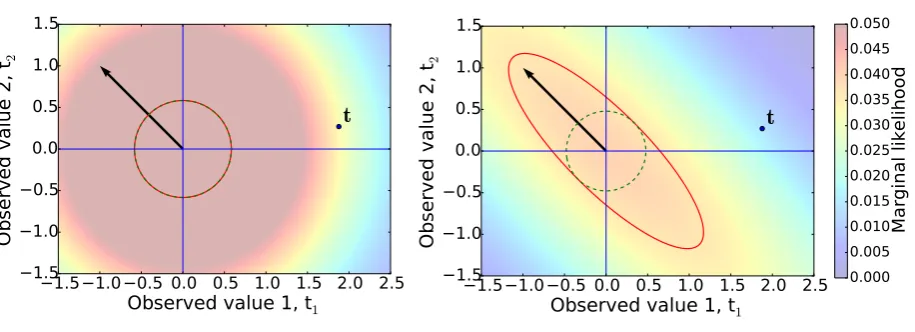
If a covariance matrix associated to a basis function is poorly aligned with the experimental observation vectort, then any finiteαvalue will lower the value of the density att. This is illustrated in Fig. 1, which shows the marginal likelihood using a simple case with only one basis function, and two observations [28, 26]. The two training data are generated from a function f =sin(x)+εwithε ∼ N(x|0,1)at pointsπ/2andπ. The single basis function of the model is fb =cos(2x). In this case, any finite value ofαwill lower the marginal probability attwith respect
1.5 1.0 0.5 0.0 0.5 1.0 1.5 2.0 2.5
Observed value 1, t1
1.5
1.0
0.5
0.0
0.5
1.0
1.5
Ob
se
rv
ed
va
lue
2
, t
2t
1.5 1.0 0.5 0.0 0.5 1.0 1.5 2.0 2.5
Observed value 1, t
11.5
1.0
0.5
0.0
0.5
1.0
1.5
Ob
se
rv
ed
va
lue
2
, t
2 [image:12.595.71.529.124.290.2]t
0.000
0.005
0.010
0.015
0.020
0.025
0.030
0.035
0.040
0.045
0.050
Marginal likelihood
Figure 1: Marginal likelihood function, Eq. (42), for two observation (t1,t2). The training datatare shown in the picture as a black circle. We also
show an equiprobability line of the marginal likelihood at a Mahalanobis distance of 1.5 from the origin using the covariance from Eq. (45) with
b0/(a0−1) chosen to maximize the marginal likelihood att. Left: only noise is contributing to the covariance matrix (α→ ∞). The marginal
likelihood attin this case is 0.033. Right: the covariance matrix includes a finiteα=0.2. The contrition arising from the noise term is shown as a dashed green circle. The marginal likelihood attfor this value of alpha is reduced to 0.015. Also shown is the basis vector (cos(π),cos(2π)), which is not aligned with the datatfor our choice of basis function.
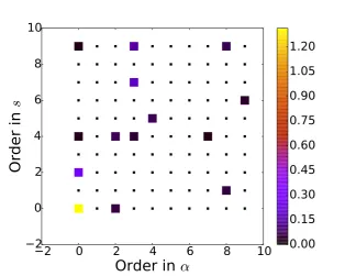
As an example of this process, Fig. 2 shows a plot of the magnitude of the regression coefficients usingS−01 = diag(α0, . . . , αM−1) for a maximum order of the modelM = Ms×Mα =10×10=100. We can see that when we
use the RVM most of the coefficients go to zero (within computer accuracy) showing that the corresponding basis functions have negligible relevance in the model.
4. Exchange Model Training
Since the value of the exchange energy is not a quantity that can be measured, we have to use other quantities for which experimental data are available. As the model is linear for the exchange energy, it is natural to choose the energy of different materials as the training data. One such energy available for a wide range of materials is the atomization energy (cohesive energy), which is the energy required for the total separation of all the atoms in the system.
Therefore, the atomization energy per atom of a system M =AnABnB. . .is defined as the sum of the energies of
the individual atoms minus the energy of the system divided by the number of atoms in the system:
Eat=
1 Na X I
nIEI−EM , (46)
whereNa =PnI is the number of atoms in the supercell andIruns over all the species of atoms, A, B,. . .EI is the
energy of the isolated atomIandEMis the energy of the systemM.
Using the decomposition of the energy defined in Eq. (2), we can write the atomization energyEatas:
Eat=
1 Na X I
nI(EbI +E x I +E
c I)−(E
b M+E
x M+E
c M) (47)
=Eatb +Exat+Ecat,
where we have defined the partial atomization energiesEatα = N1 a
P
InIEαI −EαM
2
0
2
4
6
8
10
Order in
α
[image:13.595.136.461.110.361.2]2
0
2
4
6
8
10
Or
de
r i
n
s
0.00
0.15
0.30
0.45
0.60
0.75
0.90
1.05
1.20
Figure 2: Magnitude of the coefficients obtained using a RVM for the determination of the hyperparameters. The parameters which go to zero have been plotted with a smaller symbol to highlight the sparsity of the model.
andEc
atare fixed in our model, and, using Eq. (17),Eatx can be written as
Eatx =ξT 1 Na X I
nIEx[ni;ˆe]−Ex[nM;ˆe] , (48)
whereniis the electron density of the isolated atomIandnMis the electron density of the systemM.
To obtain the parameters of the posterior distribution, Eqs. (25)-(28), we need the training data vector t with experimental data and the design matrixΦ. We build the design matrix in Eq. (29) as
Φ= 1
Na(
P I∈s1nIE
x[n
i;ˆe]−Ex[ns1;ˆe])
T
1
Na(
P I∈s2nIE
x[n
i;ˆe]−Ex[ns2;ˆe])
T
.. . 1
Na(
P I∈sNnIE
x[n
i;ˆe]−Ex[nsN;ˆe])
T , (49)
wheresiare the systems in the training data set.
Remark 7. To calculate the design matrix Eq. (49), one needs to run a self-consistent simulation to obtain the electron density for (i) every system of the training data and (ii) every isolated atom which is part of any material system in the training set.
As explained in Remark 4, the observed datatare the experimental atomization energies minus the self-consistently calculated model part not dependent on the parametersξ, i.e.
t=
Eatexp(s1)−Ebat[n1]−Eatc[n1]
Eatexp(s2)−Ebat[n2]−Eatc[n2]
.. .
Remark 8. To evaluate the exchange energy basis functionals for a systems,Ex[n
s;ˆe], one needs its electron density,
ns. Unlike the usual situation, where we know both the experimental data at a given input point where the basis are
evaluated, in our problem we do not know the electron densitya priori. Both the energy and the electron density are obtained simultaneously from a self-consistent simulation of the system. This fact, together with the high dimension-ality of the electron density field, poses problems in the application of active learning approaches for choosing the training data set.
4.1. Indirect measurements
It is possible to add other information to the training of energies indirectly to increase the size of the training set. As an example, we have included information of the experimental bulk properties for cubic materials, the equilibrium volume (V0), equilibrium bulk modulus (B0) and its pressure derivative (B1). Using their experimental values within
an equation of state (EOS), we can obtain information on the variation of the energy with the volume. One such EOS is theStabilized Jellium Equation of State(SJEOS) [29], which has the form
E(V)=a+bV 1/3 0 V1/3 +c
V02/3
V2/3 +d V0
V =γ
Tφ(V), (51)
whereVis the volume of the unit cell,γis the vector of coefficients,γ=(a,bV01/3,cV02/3,dV0), andφ(V) the vector of basis functions,φ(V)=(1,V11/3,
1
V2/3,
1
V). The coefficients of the equation are related to the equilibrium cohesive energy
(E0), equilibrium volume, bulk modulus and first derivative of bulk modulus through the following equation [29],
1 1 1 1
3 2 1 0
18 10 4 0
108 50 16 0
γ= −E0 0 9V0B0
27V0B0B1
. (52)
By isotropically straining the unit cell of a solid, we can vary its volumeV. Therefore, for every value of strain, we can obtain an energy difference with respect to the equilibrium valueV0, E(V)−E(V0). Adding this energy increment obtained for a set of five strains in the range [0.95,1.05] to the cohesive energy at equilibrium, we obtain five training points for each material (including the relaxed configuration) corresponding to cohesive energies of strained configurations.
Remark 9. Even though the errors in the energies obtained from the different sources, solids, molecules and indirect measurements will be different from each other,we have not considered it in the results presented in this work and for simplicity the same (unknown) noise is assumed for all energy data sets. This assumption can easily be relaxedusing the evidence approximation.
4.2. Training sets
To train the model, we used atomization energies of 13 cubic elemental solids from a data set of 20 cubic elemental solids (EL20) and a subset of 120 molecules from the G2/97 dataset [30]. Following the classification in Ref. [7], we have 5 solids from alkali and alkaline earth metals (K, Ca, Rb, Sr and Ba), 9 non-magnetic transition metals (V, Cu, Mo, Rh, Pd, Ag, Ta, W and Au), 5 high-coordination pblock compounds (diamond, Al, Si, Ge and Sn) and 1 magnetic material (Fe). Even though in a fully Bayesian setting we would use all the available data for the model training, we have kept a small set aside for test purposes, 2 elements from each category with more than 2 elements (K, Ca, V, Cu, C and Al) and Fe. All simulations are carried out using the projector augmented-wave (PAW) method as implemented in GPAW [31, 32, 33] using plane-wave basis. An energy cut-offof 800 eV was used throughout. For solids, Brilloin zone integrations were done on a 16×16×16 Monkhorst-Pack k-mesh [34]. Real-space relaxation of molecules in the G2/97 dataset was done using a maximum force of 0.05 eV/Å on each atom [4].
0.22 0.23 0.24 0.25 0.26 0.27 0.28 0.29
Model error standard deviation [eV/atom]
0 10 20 30 40 50 60 70 80 90
Probability
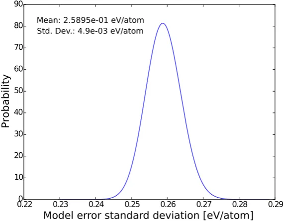
[image:15.595.150.435.131.354.2]Mean: 2.5895e-01 eV/atom Std. Dev.: 4.9e-03 eV/atom
Figure 3: Distribution of the standard deviation characterizing the likelihood function and which represents the error of the model we assume for the exchange model (meta-GGA). Its mean and standard deviation are also shown.
uncertain. This means that our functional is not expected to give reliable estimations for the exchange energy in materials very different from those included in the training data set. For example, if we have not used any magnetic material in our training set, we cannot expect our model to give accurate results for a new magnetic material. An advantage of our model including uncertainty quantification is that ideally it would give a large uncertainty for those points and this information could be used as an indicator of where we cannot have confidence in the obtained result and therefore need new training points. However, as commented in Remark 8, the way in which the input density is calculated self-consistency makes this active learning approach difficult and will not be treated further in this work.
5. Prediction of Atomization Energies
The optimization of the hyperparameters was done as outlined in Algorithm 2 using convergence thresholds
θinner =10−5% andθouter =10−4%. After training the model, we obtain a posterior distribution on the linear model
parameters according to Eq. (24),
p(ξ, β|t)=N(ξ|mN, β−1SN)G(β|aN,bN). (53)
The distribution ofβ=1/σ2, the precision of the Gaussian distribution assumed in Eq. (21), gives us an estimation of the model error for the fitted quantity, atomization energies in this case, and the larger it is the smaller the discrep-ancy between the model and the experimental values. This error is related to the model itself and will not vanish asymptotically as we increase the data set. It is more common to report this error as the standard deviationσinstead of as the precisionβ. Sinceβis given by a Gamma distribution,G(β| aN,bN), thenσ2follows an inverse Gamma
distribution [35],IG(σ2|aN,bN). Therefore,σis given by 2σIG(σ2 |aN,bN) [36]. Fig. 3 shows this distribution of
the standard deviationσ. The training gives us a value peaked at 0.16 eV for the model error of the cohesive energy. This value is smaller than the previously reported one of 0.31 eV in [7].
0
1
2
3
4
5
s
∝ |∇ |/n
4/31.0
1.2
1.4
1.6
1.8
F
x(
s,
α
=
1)
Lieb-Oxford bound
This work mBEEF MS0/PBEsol PBE TPSS MVS
0
1
2
3
4
5
α
=(
τ
−τ
W)
/τ
UEG0.80
0.85
0.90
0.95
1.00
1.05
1.10
1.15
1.20
F
x(
s
=
0
,α
)
[image:16.595.68.531.122.318.2]This work mBEEF MS0 TPSS MVS
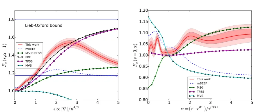
Figure 4: Exchange enhancement factors for the model developed in this work, and a series of other GGA (PBE, PBEsol) and meta-GGA (mBEEF, MS0, MVS and TPSS) functionals. The shaded regions correspond to one and two standard deviations around the average model. The left panel shows the projection onsforα=1 and the right panel the projection onαfors=0.
sfor a fixed value ofα=1 and as a function of the reduced kinetic energy densityαfor s=1. We also include the confidence intervals from coming from the distribution of parameters in Eq. (24), and other GGA (PBE and PBEsol) and meta-GGA (mBEEF, MS0, MVS [22] and TPSS) functionals.
Remark 10. The flat section aroundα=1 in the functional developed in this work, mBEEF and MS0 comes from the commonαdependence, Eq. (16), in all of them. This property is also shared by the TPSS functional. The use of anαdependence term without zero slope atα=1 could allow for more flexibility in thesdependence as shown in [22] for the “Made Very Simple” (MVS) functional.
5.1. Numerical results
The training process provided us with a predictive distribution for the exchange contribution to the atomization energy of any system outside the training set. For any new system with electron density ˜n, the predictive distribution is
p( ˜Ex|n˜,t)=St( ˜Ex|µ, λ, ν), (54)
with the parameters defined in Eqs. (31)-(33). These equations show that to obtain the parameters of the predictive distribution for the new system, we need the basis exchange energy vectorEx[˜n;ˆe]. As we did for the training of the
model, we run the simulation self-consistently using the PBE functional and construct the vectorEx[˜n;ˆe] using the
resulting density. This is then used to calculate the parameters of the Student t-distribution of the exchange energy from Eqs. (31)-(33).
Remark 11. In the training of the model, we used the self-consistent PBE densities, i.e., the densities obtained solving Eqs.(3)-(5)with the PBE XC energy functional to evaluate the basis functions (Remark 3). As a posteriori check that this is a reasonable approximation, we compare for a few systems the DFT energy using our XC func-tional with two different densities: the self-consistent density obtained using the PBE XC functional as described above, and the self-consistent density obtained with our trained model. In the first case we run a self-consistent DFT simulation using the PBE functional and keep the resulting density,nPBE. This density is then fixed and used
to obtain the average prediction of our model running a non self-consistent DFT simulation using Eq.(31)with
˜
K
Ca
V
Cu
C
Al Fe-FM
0
1
2
3
4
5
6
7
8
9
[image:17.595.137.457.109.369.2]Cohesive Energy [eV]
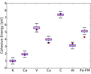
Figure 5: Box-plot of the cohesive energies of the elements in the test set. The red squares represent the experimental cohesive energies.
self-consistent DFT simulation using our average model XC energy, i.e., Eq.(18)withξgiven by Eq.(26). We will denote this energy asEsc. We found that the absolute difference betweenEnsc−PBEandEscwas below1meV, which
is lower than the typical energy resolution in DFT applications.
To evaluate the quality of the average predictions and compare it to other values found in the literature, we use the mean absolute error (MAE) and the mean absolute relative error (MARE). For a set of calculated dataxcalc ={xcalc
i }
and the corresponding set of experimental dataxexp={xexp
i }, the MAE and MARE of the calculations are defined as:
MAE= 1 N
N X
i=1
|xcalci −xexpi |, (55)
MARE= 1 N
N X
i=1
xcalci −xexpi xexpi
. (56)
Figure 5 shows a box-plot of the distributions of cohesive energies of the elements in the EL20 test set together with the experimental values. Except for Fe, all experimental points fall within the confidence interval given by our model. Fe is a magnetic material, which is a family not represented in our training set and therefore we can expect that the results for it will not be predictive. Also, we must bear in mind that for some magnetic elements the thermal extrapolations to 0 K used on the experimental data are no longer valid [7].
Remark 12. As discussed on Section 3.1, the predictions from the model are correlated. As an example of this effect, we calculate the uncertainty in the difference between the cohesive energies of K and Ca. The predicted values for both materials are1.015±0.165 and1.945±0.166 eV, respectively. The cohesive energy difference ignoring correlations, i.e., just subtracting the two random variables as obtained from Eq.(30), is0.930±0.234
eV, whereas if we include correlations, i.e., subtracting the two correlated variables as obtained from Eq.(37), it is
[image:17.595.240.362.505.567.2]XC functional Error G2/97-test G2/97 EL20-test EL20
This work MAE 0.116 0.103 0.243 0.0975
MARE 3.27 1.46 8.56 5.62
PBE MAE 0.703 0.238
[image:18.595.155.440.214.326.2]MARE 5.09 6.88
Table 1: Mean absolute error (in eV) and mean absolute relative error (in %) of the predictions of atomization energies using the average model for the training sets containing molecules (G2/97) and solids (EL20).
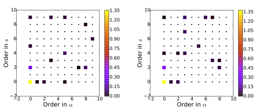
C functional Error G2/97-test G2/97 EL20-test EL20
PBE MAE 0.116 0.103 0.243 0.0975
MARE 3.27 1.46 8.56 5.62
PBEsol MAE 0.116 0.108 0.204 0.172
MARE 2.91 1.55 6.12 4.98
vPBE MAE 0.110 0.107 0.226 0.184
MARE 2.72 1.41 6.45 5.17
TPSS MAE 0.108 0.104 0.227 0.190
MARE 2.68 1.42 6.85 5.53
Table 2: Mean absolute error (in eV) and mean absolute relative error (in %) of the predictions of atomization energies using the average model with different correlation functionals.
Table 1 summarizes the MAE and MARE of the atomization energies of the elements in the EL20 and G2/97 data sets and compares them to the ones obtained with the PBE functional. The MAE for the G2/97 data set goes down from 0.703 to 0.103 eV, which was partly expected as the PBE functional does not work particularly well with molecules [4, 22]. Furthermore, our results are better than those of BEEF-vdW (0.16 eV, GGA with van de Waals corrections), TPSS (0.28 eV) or the hybrid functionals B3LYP (0.14 eV) and PBE0 (0.21 eV) [4]. On the other hand, the performance in our solids data set shows very similar results for both functionals.
To further study the predictive capabilities of the functional, we tested it on 37 molecules from the G3-3 subset of the G3/99 data set [37]. The MAE and MARE were found to be 0.0608 eV and 0.11%, respectively. Even though it is only half of the complete G3-3 set, the MAE is less than half of the best reported in Ref. [4] for the whole data set, including LDA, GGA, meta-GGA and hybrid exchange correlation functionals.
5.2. Impact of different correlation functionals
Since the correlation part of the functional is not trained, we tried four different ones to see the impact on the results: Ec
PBE,E c PBE sol,E
c
vPBE[16, 22] andE c
T PS S. Table 2 shows a comparison of the errors using the three
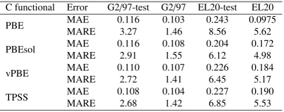
correla-tions. Even though the coefficients selected by the RVM are different, as shown in Fig. 6, the error in the predictions is similar. The vPBE correlation seems to give the best results for the molecules in the test set whereas PBEsol is the best for the test set of solids, even though both of them are outperformed by the PBE correlation if training solids are also included.
6. Propagation of Uncertainty to Derived Quantities
6.1. Lattice constant and bulk modulus of cubic materials
For cubic materials, where the volume depends on only one parameter, we can easily obtain the equilibrium lattice constant and bulk modulus from a fit of computed energies at different volumes to an EOS. We use again the SJEOS as defined in Eq. (51),
E(V)=a+bV 1/3 0 V1/3 +c
V02/3
V2/3 +d V0
V =γ
Tφ(V). (57)
The regression coefficients are related to the equilibrium energy (E0), equilibrium volume (V0), bulk modulus (B0)
2
0
2
4
6
8
10
Order in
α
2
0
2
4
6
8
10
Or
de
r i
n
s
0.00
0.15
0.30
0.45
0.60
0.75
0.90
1.05
1.20
1.35
2
0
2
4
6
8
10
Order in
α
2
0
2
4
6
8
10
Or
de
r i
n
s
[image:19.595.65.532.122.311.2]0.00
0.15
0.30
0.45
0.60
0.75
0.90
1.05
1.20
1.35
Figure 6: Magnitude of the coefficients obtained using a RVM for the determination of the hyperparameters using the PBEsol (left) and vPBE (right) correlation functionals.
To obtain their values with their associated uncertainty we proceed as follows. For each material, we run a self-consistent simulation for a set of different strains (5 points from 95% to 105% of the experimental volume) using our XC functional defined in Eq. (17) with the average values for the coefficients as defined in Eq. (26). We draw samples from the distribution in Eq. (24), and run simulations non self-consistently using the density from the self-consistent simulations. For each sample coefficients, we fit the resulting energies to the SJEOS.
Once again we use Bayesian linear regression for the process, but this time we take the error in the observed quantity (the DFT energy in this case) as given. This is related to the energy accuracy, e.g., from convergence in mesh spacing, k-points, energy cut-off, etc., and adds an extra source of uncertainty. If we assume it to be Gaussian, for each sample of XC functional coefficients the likelihood is [26]:
L(E|V,γ, β)=Y
n
N(En|γTφ(Vn), δ−1)=N(E|γTφ, δ−1I), (58)
whereδrepresents the noise in the data.
Using a Gaussian as a prior for the regression coefficients,p(γ)=N(γ|m0,S0), the posterior for the coefficients
is again a Gaussian [26],
p(γ|E)=N(γ|mN,SN), (59)
where now the mean and covariance of the posterior distribution over the parametersγare given by [26]:
mN=SN n
S−01+δΦTEo, (60)
SN=S−01+δΦ
TΦ. (61)
Using a Monte Carlo method once more, we sample the regression coefficients and invert Eq. (52) to obtainE0,V0,
Algorithm 3Calculation of uncertainty forV0andB0.
1: Input: systemswith unit cell defined by three vectorsx1,x2,x3. 2: Input:Nmax
1 ,N
max
2 , the maximum number of iterations for Monte Carlo sampling. 3: for5 strains 0.95≤σi≤1.05do
4: Strain the unit cell of the systemsbyσi:xα→σixα,α=1,2,3.
5: Self-consistent simulation of the strained system usingξ=mN.
6: Keep the self-consistent electron densityn∗i =n(σi).
7: end for 8: N1=0
9: repeat 10: SampleξN
1,βN1from Eq. (24).
11: Non self-consistent simulation usingξN
1,βN1using a fixed densityn
∗
i.
12: N2=0 13: repeat
14: SampleγN2from Eq. (59).
15: CalculateV0,B0inverting Eq. (52).
16: untilN2=Nmax
2 17: N1=N1+1
18: untilN1=Nmax
1
19: Collect statistics on calculatedV0,B0.
6.2. Prediction of bulk properties
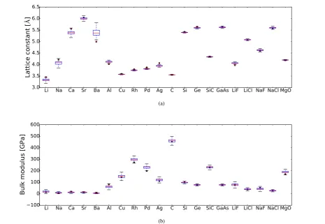
To test the bulk properties we use the SL20 test set [34] since there are available data for other XC functional to compare the performance [34, 22]. It consists of 13 elemental solids (Li, Na, Ca, Sr, Ba, Al, Cu, Rh, Pd, Ag, C, Si, Ge) and binary I-VII (LiF, LiCl, NaF, NaCl), II-VI (MgO), III-V (GaAs) and IV-IV (SiC) compounds. Note that 7 of the elemental solids in the set were used in the training of the model.
Figure 7(a) shows a box-plot of the calculated lattice constants for the elements in the set. Among the elemental solids, we see that the predictive error bars are largest for the group II elements (Ca, Sr, Ba), which together with Li have the largest absolute errors. Among the compounds, LiF has the largest error, but bearing in mind that no ionic solids were included in the training set the predictions are remarkably good, especially when poor results have been reported before with other functionals for this family of elements [38, 34].
The MAE and MARE of the predicted average lattice constants are 0.072 Å and 1.60%, respectively. The MAE is worse than other solid oriented density functionals such as PBEsol (0.036 Å) [22] and comparable to chemistry oriented semi-local functionals such as M06-L, which has a MAE of 0.071 Å, but without Ca, Sr and Ba [38, 16], which contribute importantly to the error with our functional. The mean signed error (MSE) we obtain is−0.0081 Å, which implies on average an underestimation of the lattice constants similar to the PBEsol functional but opposite to other meta-GGA functionals such as TPSS [34].
Figure 7(b) shows a box-plot of the predicted bulk modulus for the materials in the SL20 test set. The MAE and MARE of the predicted average bulk moduli are 9.71 GPa and 13.07%, respectively. These values are similar to those for other functionals such as, e.g., PBE (10.5 GPa) or TPSS (7.942 GPa) [34]. The MSE of 5.19 GPa, means that on average there is an overestimation of the bulk moduli the same as the PBE functional but opposite to the PBEsol or TPSS functionals [34].
6.2.1. Impact of the simulation convergence error
Li Na Ca Sr Ba Al Cu Rh Pd Ag C Si Ge SiC GaAs LiF LiCl NaF NaCl MgO
3.0
3.5
4.0
4.5
5.0
5.5
6.0
6.5
La
tti
ce
co
ns
ta
nt
[
]
(a)
Li Na Ca Sr Ba Al Cu Rh Pd Ag C Si Ge SiC GaAs LiF LiCl NaF NaCl MgO
100
0
100
200
300
400
500
Bulk modulus [GPa]
[image:21.595.66.532.238.570.2](b)
Li Na Ca Sr Ba Al Cu Rh Pd Ag C Si Ge SiC GaAs LiF LiCl NaF NaCl MgO
3.0
3.5
4.0
4.5
5.0
5.5
6.0
6.5
La
tti
ce
co
ns
ta
nt
[
]
(a)
Li Na Ca Sr Ba Al Cu Rh Pd Ag C Si Ge SiC GaAs LiF LiCl NaF NaCl MgO
100
0
100
200
300
400
500
600
Bulk modulus [GPa]
[image:22.595.66.532.253.574.2](b)
The widening of the error bars for the materials with high error is a proof of the ability of the proposed functional to predict the uncertainty in its predictions.
6.3. Prediction of the energy band gap of Si
As a further example of uncertainty propagation we show the calculation of the energy band gap for a semicon-ductor, Si. Kohn-Sham DFT cannot reproduce the band gap of materials properly as a consequence of the lack of a discontinuity in the XC energy functional with the number of electrons [39]. This can be overcome with the intro-duction of energy dependent XC potential [39]. An equivalent to this energy dependent XC potential can be achieved using many-body perturbation theory (MBPT), which provides a different approach to obtain the band gap. Its first order approximation, Hedin’sGW approximation [40] is already a more accurate approach to tackle the band gap problem. In this framework, XC effects are included in the energy dependent self-energy, which is a convolution of the Green’s functionGand a dynamically screened Coulomb interactionW. The obtained energies correspond to
quasiparticles(QP) describing the screened electrons and in this case the valence band maximum and conduction band minimum can be interpreted directly as the ionization potential and electron affinity in photoemission experiments and therefore can be used to calculate the experimentally measured band gap [41].
One further approximation which has been successful in calculating the band-gaps for small gap semiconductors is theG0W0approximation [42, 41], which calculates theGWQP energies perturbatively on top of the one-particle Kohn-Sham (KS) orbitals and orbital energies. Therefore, in this approximations, the QP energy spectrum is directly linked to the DFT starting point. The eigenvalues obtained as perturbations to the Kohn-Sham (KS) orbital energies are
εGW nk =ε
KS nk +
D
ψKS
nk |Σ−Vxc |ψKSnk
E
, (62)
whereεnk andψnk are the orbital energies and orbitals for bandnand wave vectork,Σis the self-energy from the
G0W0approximation andVxcthe exchange correlation energy from DFT. All calculations are done as implemented in
GPAW [43]. Since the correction depends on the KS orbitals and the XC potential, the results will depend on which XC functional is used as the initial approximation, and we will use this a measure of uncertainty for theG0W0/meta−GGA
approximation to the band structure. For each realization of our XC functional we obtain self-consistently the orbitals and their energies on a 12×12×12 Monkhorst-Pack mesh and from them theG0W0eigenvalues using Eq. (62). We estimate the band gap as the distance between the maximum of the highest occupied band and the minimum of the lowest unoccupied band. The variability in the band gap computed this way is shown in Fig. 9 together with the band gaps obtained directly from DFT. We can see that both approaches have a similar absolute value of the uncertainty in the band gap, even though the values obtained with theG0W0approximation are, as expected, much more accurate.
7. Summary and Conclusions
We have presented a new approach based on machine learning using a Bayesian framework to obtain an exchange-correlation energy functional. In this way, the coefficients of the functional are not point estimates, but random variables, so that the resulting exchange-correlation functional is also a random variable, even though the model exchange energy basis are fixed. Imposing certain assumptions in the training process, we obtained an analytical expression for the distribution function of the model parameters. Having a random variable instead of a point estimate allows for the quantification of uncertainty in the simulation results. Uncertainties in the predictions will include limited data uncertainty, i.e., uncertainty in the training process due to the availability of limited training data, and model uncertainty, i.e., uncertainty due to the inability of the proposed model to reproduce the experimental data. Limited data uncertainty could in principle be reduced asymptotically to zero as the number of training data increases. However, our model uncertainty would not vanish in the limit of infinite basis functions as the framework we are using (meta-GGA XC functional) is intrinsically limited.
Whereas previous approaches using empirical models for the XC energy, i.e., models which fit their coefficients to experimental data, have used a fixed functional dependence, which limits the number of basis functions as they lend themselves to overfitting, we use a relevance vector machine. This means that during the training process there is an automatic model selection trough the sparsification of the model coefficients, which reduces the risk of overfitting.
0.0
0.5
1.0
1.5
2.0
Band gap [eV]
0.0
0.5
1.0
1.5
2.0
2.5
3.0
P
ro
b
a
b
il
it
y
Exper.
Mean
G
0W
0 [image:24.595.128.466.267.536.2]Mean KS
Figure 9: Histograms of the band gap of Si using KS-DFT (grey) and theG0W0approximation (red) with our XC functional. Gaussian fits are
also shown as a guide to the eye. The black vertical line corresponds to the experimental value, the red vertical line to theG0W0band gap with the
![Figure 7: Box-plot of the (a) equilibrium lattice constants and (b) equilibrium bulk moduli of the elements in the SL20 test set [34]](https://thumb-us.123doks.com/thumbv2/123dok_us/9463942.452913/21.595.66.532.238.570/figure-box-equilibrium-lattice-constants-equilibrium-moduli-elements.webp)