ISSN Online: 2327-4379 ISSN Print: 2327-4352
DOI: 10.4236/jamp.2019.73038 Mar. 13, 2019 527 Journal of Applied Mathematics and Physics
Solving the Linear Oscillatory Problem without
Damping with Random Loading Condition
Using the Decomposition Method
Amnah S. Al-Juhani
*, Aleh A. Al-Shammari
Faculty of Science, Tabuk University, Tabuk, KSA
Abstract
In this paper we study the solution of random linear oscillatory equation
( )
2 ;
x w x F t+ = ω
without damping and with random leading condition us-ing the method. Finally, the time evolution of the mean, variance and standard deviation has been plotted for a range of values of the natural frequency w.
Keywords
Linear Stochastic Differential Equations, Adomian Decompositions, Linear Oscillatory, Mathematica
1. Introduction
The Adomian decomposition technique was firstly introduced by Adomian in 1975. This technique can be used to solve differential, integral, algebraic and many other equations (linear or nonlinear) [1]-[12]. The method is based on a suggestion by Adomian G. that the solution can be decomposed into compo-nents. In the coming sections we will see that the Adomian decomposition me-thod is also very convenient computationally and offers some significant advan-tages [13]-[20]. The Adomian decomposition method is not a perturbation pro-cedure, so no assumption concerning the size of randomness is necessary, where each term from the decomposed solution depends only on the preceding terms. A little work in the convergence of the procedure had been done [21] [22] [23] [24] [25].
2. Problem Formulation
In this paper, we focus on solving the following Solving the linear oscillatory problem
How to cite this paper: Al-Juhani, A.S. and Al-Shammari, A.A. (2019) Solving the Linear Oscillatory Problem without Damp-ing with Random LoadDamp-ing Condition UsDamp-ing the Decomposition Method. Journal of Applied Mathematics and Physics, 7, 527-535. https://doi.org/10.4236/jamp.2019.73038
Received: April 2, 2018 Accepted: March 10, 2019 Published: March 13, 2019
Copyright © 2019 by authors and Scientific Research Publishing Inc. This work is licensed under the Creative Commons Attribution International License (CC BY 4.0).
http://creativecommons.org/licenses/by/4.0/
DOI: 10.4236/jamp.2019.73038 528 Journal of Applied Mathematics and Physics
( )
2 ;
x w x F t+ =
ω
(1)
(
;)
( )
1(
;)
F tω =e t +εn t ω (2) under stochastic excitation
F t
( )
;
ω
with the deterministic initial conditions( )
0
0,
( )
0
0x
=
x
x
=
x
where
w: frequency of oscillation,
ε
: deterministic nonlinearity scale,(
, ,P)
ω∈ Ωσ : a triple probability space with Ω as the sample space, where
σ is a σ-algebra on event in Ω and P is a probability measure, and
n t
( )
;
ω
is a white noise with the following properties:( )
;
0
En t
ω =
(3)(
1;) (
2;)
cov( ) ( )
1 , 2(
1 2)
En t ω ⋅n t ω = n t n t =δ t t− (4)
By obtaining the P.d.f. of
x t
( )
, the average and variance of the solution process in terms of t: time, the general solution is( )
0(
) ( )
0
0
1
cos x sin tsin ; d
x t x wt wt w t s F s q s
w
ω
= + +
∫
− (5)The ensemble average is given by
( )
( )(
) ( )
(
) ( )
0 0 0 0 0 0 1cos sin sin ; d
1
cos sin sin d
t
x t
t
x
Ex t x wt wt w t s EF s q s
w w
x
x wt wt w t s e s s
w µ ω = = + + − = + + −
∫
∫
(6)
The covariance takes the form
( ) ( )
(
)
(
( )
( ))
(
( )
( ))
(
)
(
) ( )
1 2
1
1 2 1 2
2 2 1 2 2 0 cov ,
sin sin d
x t x t t
x t x t E x t x t
w t s w t s e s s
w
µ
µ
ε
= − ⋅ −
=
∫
− − (7)The variance is
( )
2(
) ( )
2 2 2
2 0
sin d
t
x t w w t s e s s
ε
σ
=∫
− (8) Due to linearity and the deterministic properties of x x0,0 and the frequencyw we obtain a Gaussian solution process:
( ) ( ) ( ) ( ) ( ) 2 1 2 1 e 2π x t x t x t x t x t f µ σ
σ
− − = (9)
where ( ) 0 0
(
) ( )
0
1
cos sin tsin d
x t
x
x wt wt w t s e s s
µ
ω
ω
DOI: 10.4236/jamp.2019.73038 529 Journal of Applied Mathematics and Physics
( )
(
) ( )
2
2 2 2
2 0
sin d
t
x t w w t s e s s
ε
σ
=∫
−Equation (9) represents a closed form solution of problem (1) with random loading condition.
3. The Adomian Decomposition Method
Case-study:Let us consider
( )
; et( )
;F tω = − +εn tω (10)
In the Adomian decomposition method, differential operators are decom-posed. Thus Equation (1) is rewritten in the following form:
(
L R x F t q
+
)
=
( )
;
(11) where:2
2 2
d and
d
L R
t
ω
= =
Hence,
( )
;
Lx F t q Rx
=
−
(12)Solving for x we obtain
( )
( )
1 ; 1
x L F t q= − −L Rx− +
φ
t (13)where
φ
( )
t
is the solution of Lx=02 2
d
0 0
d x
Lx x at c
t
= ⇒ = ⇒ = + (14)
Subject to the initial conditions:
( )
t x0 x t0φ = + (15) Thus, the solution of equation takes the form:
( )
2( )
0 0
0 0 0 0
; d d d d
t t t t
x x= +x t +
∫∫
F t q t t w−∫∫
x t t t (16) We now assume that the solution can be written in the following form:( )
( )0( )
( )1( )
( )( )
0
i i
x t x t x t ∞ x t
=
= + +=
∑
(17) Substituting (17) in (16) we obtain:( )
( )
2 ( )( )
0 0
0 0 0 00 0
; d d d d
t t t t
i i
i x x x t F t q t t i x t t t
ω
∞ ∞
= =
= + + −
∑
∫ ∫
∑
∫ ∫
(18)By matching the boundaries, we obtain:
( )0
( )
( )
0 0 0 0
; d d
t t
DOI: 10.4236/jamp.2019.73038 530 Journal of Applied Mathematics and Physics
( )1
( )
2 ( )00 0
d d
t t
x t = −w
∫∫
x t t (20) ( )2( )
2 ( )1( )
0 0
d d
t t
x t = −w
∫∫
x t t t (21)And the nth term will be:
( )
( )
2 ( )1( )
0 0
d d , 1
t t
n n
x t = −w x − t t t n≥
∫∫
(22) By applying this procedure to equation, we obtain:( )1
( )
2 2 2 3 2 1 1( )
0 ;
2! 3!
ot t
x t = −w x −w x −w L L F t q− − (23)
( )2
( )
4 4 4 5 4 1 1 1( )
0 0 ;
4! 5!
t t
x t =w x +w x +w L L L F t q− − − (24)
( )3
( )
6 6 6 7 6( )
1 4( )
06!t 07!t ;
x t = −w x −w x −w L− F t q (25)
( )4
( )
8 8 8 9 8( )
1 5( )
0 0 ;
8! 9!
t t
x t =w x +w x +w L− F t q (26)
The nth term is:
( )
( )
(
)
( )
( )
2 2 1 1
2 2 2 1
02 ! 0 2 1 ! ;
n n n
n n t n t n
x t w x w x w L F t q
n n
+ +
−
= + +
+
(27)
Thus,
( )
( ) ( ) ( )( ) ( )
( ) ( ) ( )
( )
( )
( )
( )
( )
( )
( )
0 1 2
2 4 3 5
0 0
2 3 4 5
1 3 1 5 1 7 1 9 1
2 1 2 1 0
0
1
2! 4! 3! 5!
1 ;
1
cos sin ;
x t x x x
wt wt x wt wt
x wt
wL w L w L w L w L F t q
w
x
x t t L L F t q
ω
ω ω ω ω
ω ω − − − − − − − = + + + = − + + + − + + + − + − + + = + + − (28) where,
( )
(
(
)
)
1( )
0 0 0
d d
1 ! n
t t t
n t u
F u u F u u
n
−
− =
−
∫ ∫
∫
(29)( )
( )
(
) ( )
1 2
0 0 0
; t t ; d t ; d
L F t q− = F t q t = t u F u q u−
∫∫
∫
(30)( )
( )
(
) ( )
31 1 4
0 0 0 0 0
; ; d ; d
3!
t t t t t t u
L L F t q− − = F t q t = − F u q u
∫ ∫ ∫ ∫
∫
(31)( )
( )
(
) ( )
51 1 1 6
0 0 0 0 0 0 0
; ; d ; d
5!
t t t t t t t t u
L L L F t q− − − = F t q t = − F u q u
DOI: 10.4236/jamp.2019.73038 531 Journal of Applied Mathematics and Physics
Figure 1. The mean of x t
( )
at ω =1.Figure 2. The variance of x t
( )
at ω =1.DOI: 10.4236/jamp.2019.73038 532 Journal of Applied Mathematics and Physics
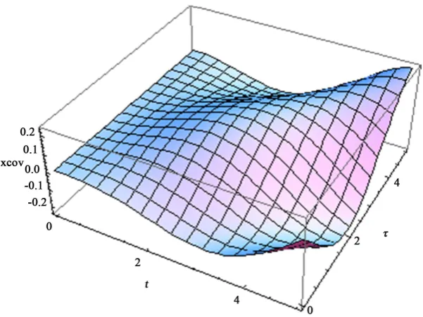
[image:6.595.223.524.68.293.2]Figure 4. The covariance of x t
( )
at ε=0.3,ω=1.Figure 5. The mean of x t
( )
at ω =0.5. [image:6.595.209.535.88.729.2]DOI: 10.4236/jamp.2019.73038 533 Journal of Applied Mathematics and Physics
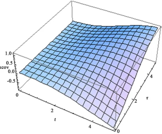
[image:7.595.242.507.292.511.2]Figure 7. The covariance of x t
( )
at ε=0.1,ω=0.5.Figure 8. The covariance of x t
( )
at ε=0.3,ω=0.5.( )
(
) ( )
(
) ( )
(
) ( )
(
) ( )
(
)
(
)
( )
(
) ( )
0 0
0
3 5
3 5
0 0
7 7
0
3 0
0
0
0 0
0
1
cos sin ; d
; d ; d
3! 5!
; d 7!
1
cos sin ; d
3! 1
cos sin sin ; d
t
t t
t
t
t
x
x t x wt wt w t u F u q u
w
t u t u
w F u q u w F u q u
t u
w F u q u
w t u x
x wt wt w t u F u q u
w x
x wt wt w t u F u q u
w w
ω
ω
= + + −
− −
− +
−
− +
−
= + + − − +
= + + −
∫
∫
∫
∫
∫
∫
DOI: 10.4236/jamp.2019.73038 534 Journal of Applied Mathematics and Physics
Example: Let us consider
( )
;( )
1( )
;F t ω =e t +εn t q (34) in the previous case-study. By using the decomposition method, the following results are obtained (Figures 1-8).
References
[1] Rubinstein, R. and Choudhari, M. (2005) Uncertainty Quantification for Systems with Random Initial Conditions Using Wiener-Hermite Expansions. Studies in Ap-plied Mathematics, 114, 167-188.https://doi.org/10.1111/j.0022-2526.2005.01543.x
[2] He J.H. (1999) Homotopy Perturbation Technique. Computer Methods in Applied Mechanics and Engineering, 178, 257-292.
https://doi.org/10.1016/S0045-7825(99)00018-3
[3] Nayfeh, A. (1993) Problems in Perturbation. Wiley, New York.
[4] Tamura, Y. and Nakayama, J. (2005) Enhanced Scattering from a Thin Film with One-Dimensional Disorder. Waves in Random and Complex Media, 15, 269-295. https://doi.org/10.1080/17455030500053336
[5] Jahedi, A. and Ahmadi, G. (1983) Application of Wiener-Hermite Expansion to Non-Stationary Random Vibration of a Duffing Oscillator. Journal of Applied Me-chanics, Transactions ASME, 50, 436-442.https://doi.org/10.1115/1.3167056
[6] Orabi and Ismail, I. (1988) Response of the Duffing Oscillator to a Non-Gaussian Random Excitation. Journal of Applied Mechanics, Transaction of ASME, 55, 740-743.https://doi.org/10.1115/1.3125861
[7] Kayanuma, Y. and Noba, K. (2001) Wiener-Hermite Expansion Formalism for the Stochastic Model of a Driven Quantum System. Chemical Physics, 268, 177-188. https://doi.org/10.1016/S0301-0104(01)00305-6
[8] Kenny, O. and Nelson, D. (1997) Time-Frequency Methods for Enhancing Speech
Proceedings of SPIE—The International Society for Optical Engineering, 3162, 48-57.
[9] De Feriet, K. (1955) Random Solutions of Partial Differential Equations. 3rd Berke-ley Symposium on Mathematical Statistics and Probability, Vol. III, 199-208. [10] El Tawil, M. (1990) On Stochastic Partial Differential Equations. AMSE Review, 14,
1-8.
[11] El-Tawil, M. and Saleh, M. (1998) The Stochastic Diffusion Equation with a Ran-dom Diffusion Coefficient. Ain Shams Engineering Journal, 33, 605-613.
[12] Mckean (1969) Stochastic Integrals. Academic Press, New York.
[13] Kloeden, P.E. and Platen, E. (1992) Numerical Solution of Stochastic Differential Equations. Springer-Verlag, Berlin. https://doi.org/10.1007/978-3-662-12616-5
[14] Arnold, L. (1974) Stochastic Differential Equation Theory and Applications. John Wiley, New York.
[15] Adomian, G. (1988) A Review of the Decomposition in Applied Mathematics. Ma-thematical Analysis and Applications, 135, 501-544.
https://doi.org/10.1016/0022-247X(88)90170-9
DOI: 10.4236/jamp.2019.73038 535 Journal of Applied Mathematics and Physics
[17] Ahmed, A. (2008) Adomian Decomposition Method: Convergence Analysis and Numerical Approximations. Msc, McMaster University, Hamilton.
[18] Johan, G.J. and Snell, I. (1976) Finite Markov Chains. Springer-Verlag, New York. [19] Harold, J. (1977) Probability Methods for Approximation in Stochastic Control for
Elliptic Equation. Academic Press, New York.
[20] Papoulis, A. (1984) Probability, Random Variables, and Stochastic Processes. McGraw-Hill, New York.
[21] Robert, B. and Melvin, F. (1975) Topics in Stochastic Processes. Academic Press, New York.
[22] Yong, Y. (1995) Convergence of Adomian Method and a Lgorithm for Adomian Polynomials.Journal of Mathematical Analysis and Applications, 33, 442-449. [23] El-Tawil, M., et al. (2002) Decomposition Solution of Stochastic Nonlinear
Oscilla-tor. International Journal of Differential Equations, 6, 441-422.
[24] El-Tawil, M. and Al-Jihany, A. (2009) Approximate Solution of Mixed Nonlinear Stochastic Oscillator. Computers & Mathematics with Applications, 58, 2236-2259.
https://doi.org/10.1016/j.camwa.2009.03.057