Model-free POMDP optimisation of tutoring systems with echo-state
networks
Lucie Daubigney1,3 Matthieu Geist1
1IMS-MaLIS – Sup´elec (Metz, France),2UMI2958 – GeorgiaTech/CNRS (Metz, France) 3Team project MaIA – Loria (Nancy, France)
Olivier Pietquin1,2
Abstract
Intelligent Tutoring Systems (ITSs) are now recognised as an interesting alter-native for providing learning opportuni-ties in various domains. The Reinforce-ment Learning (RL) approach has been shown reliable for finding efficient teach-ing strategies. However, similarly to other human-machine interaction systems such as spoken dialogue systems, ITSs suffer from a partial knowledge of the interlocu-tor’s intentions. In the dialogue case, en-gineering work can infer a precise state of the user by taking into account the uncer-tainty provided by the spoken understand-ing language module. A model-free ap-proach based on RL and Echo State New-torks (ESNs), which retrieves similar in-formation, is proposed here for tutoring.
1 Introduction
For the last decades, Intelligent Tutoring Sys-tems (ITSs) have become powerful tools in various domains such as mathematics (Koedinger et al., 1997), physics (Vanlehn et al., 2005; Litman and Silliman, 2004; Graesser et al., 2005), computer sciences (Corbett et al., 1995), reading (Mostow and Aist, 2001), or foreign languages (Heift and Schulze, 2007; Amaral and Meurers, 2011). Their appeal relies on the fact that each student does not have to follow an average teaching strategy, espe-cially as the one-to-one tutoring has been proven the most efficent (Bloom, 1968). The expertise of a teacher relies on his capacity to advice at the right time the student to acquire new skills. To do so, the teacher is able to choose iteratively ped-agogical activities. From this perspective, teach-ing is a sequential decision-makteach-ing problem. To solve it, the reinforcement learning (Sutton and Barto, 1998) approach and the Markov Decision
Process (MDP) paradigm have been successfully used (Iglesias et al., 2009). Given a situation, each teacher’s decision is locally quantified by a re-ward. However, the consequences of the teacher’s actions on the student’s cognition cannot be ex-actly determined, which introduce uncertainty.
To find a solution, one can notice that spoken dialogue management and tutoring are closely re-lated. Both are humain-computer interactions in which the human user’s intentions are not per-fectly known. In the spoken dialogue case, the partial observability is due to the recognition er-rors introduced by the speech understanding mod-ule. They are taken into account by using some hypotheses about how the language is constructed. Thus, accurate models to link observations from the user’s recognised utterances to the underlying intentions can be set up. For example, the Hidden Information State paradigm (Young et al., 2006; Young et al., 2010) builds a state which is a sum-mary of the dialogue history (Gaˇsi´c et al., 2010; Daubigney et al., 2011; Daubigney et al., 2012). However, in the ITS case, such a state is harder to develop since the cognition cannot be determined by analysing a physical signal. Thus, a model-free approach is preferred here.
To do so, a memory of the past observations and actions is built by means of a Recurrent Neu-ral Network (RNN) and more precisely an Echo State Network (ESN) (Jaeger, 2001). The inter-nal state of the network can be shown (under some resonable conditions) to meet the Markov prop-erty (Szita et al., 2006). This internal state is then used with a standard RL algorithm to estimate the optimal solution. It has already been applied to RL in (Szita et al., 2006) in limited toy applications and it is, to our knowledge, the first attempt to use it in an interaction framework. The proof of con-cept presented in Szita’s article uses the common SARSA algorithm which is an on-line and on-policyalgorithm. Each improvement of the
egy is directly tested. In the case of teaching, test-ing poor decisions can be problematic. Here, we thus propose the combination of an ESN with an
off-lineandoff-policyalgorithm, namely the Least Square Policy Algorithm (LSPI) (Lagoudakis and Parr, 2003), which is another original contribu-tion of this paper. Indeed, learning the solucontribu-tion with Partially Observable MDPs in a batch and off-policy manner is not common in the literature.
2 Markov Decision Process and Reinforcement Learning
Formally, an MDP is a tuple {S, A, T, R, γ} set up to describe the tutor environment. The set S is the state space which represents the infor-mation about the student, A is the action space which contains the tutor’s actions, T is a set of
transition probabilities defined such that T =
{p(s0|s, a),∀(s0, s, a) ∈ S × S ×A}, R is the
reward function, given according to the student progression for example, and γ ∈ [0,1] is the
discount factorwhich weights the future rewards. The set of transitions probabilities in the ITS case is unknown: the evolution of the student intentions cannot be determined. Solving the MPD consists in finding the optimal strategy, called the optimal policy which brings the highest expected cumula-tive reward.
However, in the ITS case, information about the student’s knowledge, represented by s, can only be known through observations. LetO ={oi}be the set of possible observations. Yet, if only ob-servations are available, a memory of what hap-pened during previous interactions (the history) is necessary, because the process of observations does not meet the Markov property. The his-tory is the sequence of observation-action pairs encountered during a whole teaching phase. Let H ={hi}be the set of all possible histories with hi ={o0, a0, o1, a1, ..., oi−1, ai−1, oi}.
When the POMDP framework is used, the un-derlying state si is inferred from the history by means of a model of probabilities linking si to hi. In the case of human-machine interactions, this model is not available. It can be approximated but the considered solutions aread-hocto a particular problem, thus difficult to reuse. Here, we propose an approach with as few assumptions as possible about the student cognitive model by using Echo States Networks (ESNs). This approach builds a compact representation of the history spaceH.
u0
u1
u2
Input
x0
x1
x2
x3
x4 x
5
x6
x7 x
8
x9
Reservoir
y0
y1
y2
y3
Output
[image:2.595.335.495.66.175.2]1
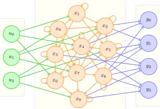
Figure 1: RNN structure (for sake of readability, all the connections do not appear).
3 Echo State Networks
An Echo State Network is represented by three layers of neurons (Fig. 1): an input, a hidden and an output. The number of neurons in the hidden layer is supposed to be large and each of them can be connected to itself. These recurrent con-nections are responsible for reusing the value of the neurons at a previous time step. Consequently, a memory is built in the reservoir and trajectories can be encoded. Only the connections from the hidden layer to the output one are learnt since all the other connections are randomly and sparsely set. The recurrent connections are defined so that the echo state property is met (Jaeger, 2001): if after a given number of updates of the input neu-rons, two internal states are exactly the same, then the input sequences which led to these two internal states are identical.
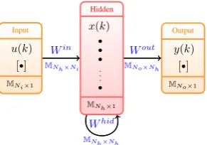
The connections of the ESN are presented in Fig. 2, with uk ∈ RNi, xk ∈ RNh and yk ∈ RNo, respectively representing the values of the input, hidden and output layers, Ni, Nh and No being the respective number of neurons and Win ∈ MNh×Ni, W
hid ∈ M
Nh×Nh and
Wout ∈ MNo×Nh, matrix containing the
synap-tic weights. After a training, the outputykreturns a linear approximation of the internal state of the reservoir. This output depends on the sequence of inputsu0,· · ·, ukand not onlyuk, throughxk.
Q-Input u(k)
[•] MNi×1
Hidden
x(k)
• • •
.. .
•
MNh×1
Output y(k) [•] MNo×1
Whid MNh×Nh
Win MNh×Ni
Wout MNo×Nh
Input u(k)
[•] MNi×1
Hidden x(k)
• • •
.. .
•
MNh×1
Projection
xΠ(k) �•
• • �
Mm×1
Output y(k) [•] MNo×1
Whid MNh×Nh
Win MNh×Ni
Π
Mm×Nh
[image:3.595.108.254.64.166.2]Wout MNo×m
Figure 2: Structure of an ESN. For the example, Ni = 1andNo = 1.
function. This function is associated with a policy π, defined for each couple (s, a) ∈ S ×A such thatQπ(s, a) = EPiγiri|s0 =s, a0 =a and
quantifies the policy. ESNs are used in the fol-lowing way to solve RL problems. The network is responsible for giving, from an observationsok and an actionakat time stepk, a linear estimation of the value of the Q-function Qˆθ(hk, ak) (with
hk = {o0, a0, ..., ok−1, ak−1, ok}). The state sis not used in the estimation of the Q-function since it is unknown. Instead, it is replaced by the history hk. The input of the ESN, uk, is thus the con-catenation of the observationokand the actionak: uk = (ok, ak). The internal state xk which com-ponent are in[−1,1], is a summary of the history
hk and the actionak. Thus, the estimation of the Q-function isQˆθ(hk, ak) = θ>x
k. The values of the output connections are learnt by means of the LSPI algorithm. With this algorithm, the optimal policy is learnt from a fixed set of data.
4 Experimental settings
For the experiments, we assume that the teaching can be done by means of three actions. First, a les-son can be presented to make the knowledge of the student increase. The second and third actions are evaluations. They can either be a simple question or a final exam. The final exam consists in ask-ing a hundred yes/no questions of equal complex-ity and on the same topic. The student does not have a feedback. Once it is proposed, a new teach-ing episode starts. Three observations are returned to the ITS. If a lesson is proposed to the user, the observation is neutral: no feedback comes from the student since the direct influence of the lesson remains unknown. The two other obervations ap-pear when a question is asked (yes or no). Conse-quently, one observation is not enough to choose the next action since no clue is given about how many lessons have led to this result. A non-null
re-ward is only given when a final exam is proposed. In this case, it is proportional to the rate of cor-rect answers among all the answers given during the exam. Thus, each improvement is taken into account. Theγfactor is set to0.97.
In this proof of concept, the results have been obtained with simulated students from (Chang et al., 2006) to ensure the reproducibility of the ex-periments. The simulation implements two abili-ties: answering a question and learning with a les-son. Three groups of students have been set up. The first one,T1, is supposed to be able to learn very efficiently, the second,T2, needs a few more
lessons to provide good answers, and the third,T3,
needs a lot of lessons to answer correctly.
5 Results
Several teaching strategies have been compared. As a lower bound baseline, a random strategy has been tested. With a probability (w.p.) of0.6, a
les-son is proposed, w.p. of0.2a question is chosen,
and w.p. of0.2a final exam is proposed. The data
generated with this random strategy have been used by the LSPI algorithm and an informed state space. The second baseline proposed is the reac-tive policy learnt by LSPI (calledreactive-LSPI), only from obervations. Neither the information about the number of lessons proposed nor the in-ternal state of the ESN is used. The third strategy is learnt by using the observations and a counter of lessons already given (called informed-LSPI). Thus, this state supposedly contains sufficient in-formation to take the decision. For this case, since the numbers of observations and lessons are dis-crete thus countable, a tabular representation is chosen for the Q-function. The fourth strategy uses the internal state of the ESN as basis function for the Q-function (calledESN-LSPI). There are
50hidden neurons. Different sizes of training data
sets are tested. Among the data, the three types of students are represented in equal proportions. One hundred policies are learnt for each of the methods presented, except for the ESN-LSPI. For this one,
10ESNs are generated and10training sessions are performed with each one of them. The mean over the average results of each of the10 learnings is
presented in the results. Each of the policies have been tested1000times.
0.3 0.4 0.5 0.6 0.7
0 2000 4000 6000 8000 10000
Average sum of discounted rewards
[image:4.595.75.286.62.208.2]Number of transitions Random Reactive-LSPI Informed-LSPI ESN-LSPI
Figure 3: Comparison of the different strategies.
the standard deviation is larger when the ESN are used because uncertainty is added when generat-ing the ESN since the connections are randomly set. The random and the reactive policies give the poorest results. Yet, the average reward in-creases because of the data in the training set. For small sets, long sequences of lessons only have not been encountered. Thus, larger rewards have not been encountered either. For the two other curves, with a reasonable number of interactions (around
8000), a good strategy is learnt by using
informed-LSPI. The strategies learnt with the ESN require fewer transitions and allow a faster learning. In this case, the optimum is reached with2000
transi-tions while8000ones are needed to reach the same
quality with the informed-LSPI strategy. Around
10000 samples, both policies give the same
re-sults. However, less information is given in the ESN approach (only observations). Thus, this ap-proach is more generic. The counter information may not be sufficient for more complex problems. To compare the efficiency of the learnt policies, the informed-LSPI and ESN-LSPI are plotted for each group of students in Fig. 4. All the strate-gies are learnt with the same data sets than pre-viously, but only one type of students is tested at a time. For theT2andT3types, the average
re-sults are better with ESN-LSPI (especially for the T3 type). For the T1 group, informed-LSPI
re-turns slighlty better results. A better insight of the behaviour of each policy is given in Fig. 5 by plotting the distribution of the actions used dur-ing the test phase. A comparison reveals that the number of lessons is higher in the ESN-LSPI case (around3) whereas only one lesson is given in
av-erage with informed-LSPI. This is of benefit to students of the third group and thus implicitly to those of the first and second groups. The number of lessons is even larger for the third group than for
0 0.1 0.2 0.3 0.4 0.5 0.6 0.7 0.8 0.9
0 2000 4000 6000 8000 10000
Average sum of discounted rewards
[image:4.595.309.521.64.209.2]Number of transitions Informed-LSPI (StudentT1) Informed-LSPI (StudentT2) Informed-LSPI (StudentT3) ESN-LSPI (StudentT1) ESN-LSPI (StudentT2) ESN-LSPI (StudentT3)
Figure 4: Results of the learnt policies for each group of students.
0 1 2 3 4
Lesson Question FinalExam
Av
g.
num
be
r o
f a
cti
ons
Actions proposed with Informed LSPI StudentT1 StudentT2 StudentT3
0 1 2 3 4
Lesson Question FinalExam
Av
g.
num
be
r o
f a
cti
ons
Actions proposed with ESN LSPI StudentT1 StudentT2 StudentT3
Figure 5: Distribution of the actions (the size of the training dataset is10000).
the two others (0.5more in average). However, in
the informed-LSPI case, the learnt policy is only profitable for those of the first group, who are al-ready skilled (this conclusion is consistent with the Fig. 4). Questions are very rarely asked because once the number of lessons has been learnt, they bring no more information.
6 Conclusion
We proposed a model-free approach which uses only observations to find optimal teaching state-gies. A summary of the history encountered is implemented by means of an ESN. This summary has been proven to be Markovian by (Szita et al., 2006). A standard RL algorithm which can learn from already collected data, is then used to per-form the learning. Preliminary experiments have been presented on simulated data. In future works, we plan to apply this method to SDSs.
Acknowledgments
[image:4.595.313.518.253.405.2]References
L. Amaral and D. Meurers. 2011. On using intelli-gent computer-assisted language learning in real-life
foreign language teaching and learning. ReCALL,
23(1):4–24.
B. Bloom. 1968. Learning for mastery. Evaluation
comment, 1(2):1–5.
K. Chang, J. Beck, J. Mostow, and A. Corbett. 2006. A bayes net toolkit for student modeling in intelligent tutoring systems. In Intelligent Tutoring Systems, pages 104–113. Springer.
A. Corbett, J. Anderson, and A. OBrien. 1995. Student
modeling in the act programming tutor. Cognitively
diagnostic assessment, pages 19–41.
L. Daubigney, M. Gaˇsi´c, S. Chandramohan, M. Geist, O. Pietquin, and S. Young. 2011. Uncertainty management for on-line optimisation of a
POMDP-based large-scale spoken dialogue system. In
Pro-ceedings of Interspeech’11.
L. Daubigney, M. Geist, S. Chandramohan, and O. Pietquin. 2012. A Comprehensive Reinforce-ment Learning Framework for Dialogue
Manage-ment Optimisation. IEEE Journal of Selected Topics
in Signal Processing, 6(8):891–902.
M. Gaˇsi´c, F. Jurˇc´ıˇcek, S. Keizer, F. Mairesse, B. Thom-son, K. Yu, and S. Young. 2010. Gaussian pro-cesses for fast policy optimisation of POMDP-based dialogue managers. InProceedings of SIGdial’10.
A. Graesser, P. Chipman, B. Haynes, and A. Olney. 2005. Autotutor: An intelligent tutoring system
with mixed-initiative dialogue. Education, IEEE
Transactions on, 48(4):612–618.
T. Heift and M. Schulze. 2007. Errors and intelligence in computer-assisted language learning: Parsers and pedagogues, volume 2. Psychology Press.
Ana Iglesias, Paloma Mart´ınez, Ricardo Aler, and Fer-nando Fern´andez. 2009. Learning teaching strate-gies in an adaptive and intelligent educational
sys-tem through reinforcement learning. Applied
Intel-ligence, 31(1):89–106.
H. Jaeger. 2001. The ”echo state” approach to
analysing and training recurrent neural networks. Technical report, Technical Report GMD Report 148, German National Research Center for Informa-tion Technology.
K. Koedinger, J. Anderson, W. Hadley, M. Mark, et al. 1997. Intelligent tutoring goes to school in the big city. International Journal of Artificial Intelligence in Education (IJAIED), 8:30–43.
M. Lagoudakis and R. Parr. 2003. Least-squares
pol-icy iteration. The Journal of Machine Learning
Re-search, 4:1107–1149.
D. Litman and S. Silliman. 2004. Itspoke: An
intel-ligent tutoring spoken dialogue system. In
Demon-stration Papers at HLT-NAACL 2004, pages 5–8. As-sociation for Computational Linguistics.
J. Mostow and G. Aist. 2001. Evaluating tutors that listen: an overview of project listen. InSmart ma-chines in education, pages 169–234. MIT Press.
R. Sutton and A. Barto. 1998.Reinforcement learning: An introduction. The MIT press.
I. Szita, V. Gyenes, and A. L˝orincz. 2006.
Reinforce-ment learning with echo state networks. Artificial
Neural Networks–ICANN 2006, pages 830–839.
K. Vanlehn, C. Lynch, K. Schulze, J. Shapiro, R. Shelby, L. Taylor, D. Treacy, A. Weinstein, and M. Wintersgill. 2005. The andes physics tutoring
system: Lessons learned. International Journal of
Artificial Intelligence in Education, 15(3):147–204.
S. Young, J. Schatzmann, B. Thomson, H. Ye, and K. Weilhammer. 2006. The HIS dialogue manager. In Proceedings of IEEE/ACL Workshop on Spoken Language Technology (SLT’06).
S. Young, M. Gasic, S. Keizer, F. Mairesse, J. Schatz-mann, B. Thomson, and K. Yu. 2010. The hid-den information state model: A practical frame-work for POMDP-based spoken dialogue
manage-ment. Computer Speech & Language, 24(2):150–