Permanent wave structures on an open two layer fluid

on an

OPEN

TWO

LAYER FLUID

by

P.J. BRYANT

No. l

_{November 1976}

PERMANENT WAVE STRUCTURES ON AN

OPEN TWO LAYER FLUID

By P.J'. Bryant

There is a significant nonlinear interaction between fast free

surface waves and slow interface waves when the group velocity of the free

surface waves is the same as the phase velocity of the interface waves.

This interaction leads to permanent wave structures consisting of a wave

group of permanent envelope on the free surface and a wave· of perma,nent

shape on the interface. A theory is developed for periodic permanent

wave structures of this type, from which solutions are found numerically.

'l'he theory includes all significant quadratic nonlinear interactions

between free surface harmonics and interface harmonics, as well as between

the interface harmonics themselves. It is found that there is a sequence

1. Introduction.

Two w1iform layers of fluid with densities of similar magnitude and a

free upper surface have two modes of gravity wave propagation, a fast free

surface wave mode and a slow interface wave mode. When both wave modes

are present, a nonlinear interaction occurs between them. Benney [l] has

shown that the nonlinear interaction is resonant when the group velocity

of the fast free surface wave mode equals the phase velocity of the slow

interface wave mode, This property leads to permanent wave structures in

which a wave group of permanent envelope on the free surface is coupled

with and moves with the same velocity as a permanent wave on the interface.

The interaction between surface waves and internal waves has been

studied previously in terms of the response of the surface waves to the

velocity field caused at the surface by the internal waves [2, 3,

4J.

The

concept of radiation stress was used to determine the behaviour of a surface

wave under the influence of a prescribed internal wave. This method is

unsatisfactory for the present problem because the shape of the internal

wave, as well as the shape of the surface wave, are unknown quantities. It

was found in these investigations that maximum interaction occurs when the

phase velocity of the internal wave and the group velocity of the surface

wave are matched.

The approach used here is to assume that the wave propagation is

unidirectional and is spatially periodic. The surface and interface waves

may then be represented by Fourier series whose coefficients have a slow

time dependence. Equations are foW1d for the time rate of change of each

Fourier amplitude in terms of all significant quadratic interactions between

all Fourier amplitudes. Solutions describing permanent wave structures are

found from these equations. In the limit as the fundamental wavelength

becomes large compared with the depth, the Fourier series tend towards

The properties of long waves on a shallow uniform

singZe

layer fluid

are dominated by the near-resonant nature of the interactions between wave

harmonics

[5, 6],

If k and l denote the wavenumbers of two long wave

harmonics propagating in the same direction with frequencies u)k, wl, then

wk + w l - wk+ l

=

O ( µ 2 ) ' ( 1. 1)

where µ is a measure of the ratio of fluid depth to wavelength. For waves

long compared with the depth, this near-resonant interaction causes the k+l

harmonic to grow to an amplitude comparable with the amplitudes of the k and

l harmonics separately. A long periodic wave therefore contains a large

number of harmonics, whose amplitudes decrease with increasing wavenumber

because their interactions move further from resonance. The long periodic

waveB of permanent form are approximated by cnoidal waves, tending towards

solitary waves as the separation between consecutive crests increases.

The same general properties are valid for single mode pennanerrt waves

in a two layer fluid. Peters & Stoker [ 7] have shown that there exist fast

free surface permanent waves and slow interface permanent waves. The near~

resonant condition (equation 1.1) then applies respectively either to the

frequencies of the fast free surface wave harmonics alone, or to the

frequencies of the slow interface wave harmonics alone.

When both wave modes are present, significant near-resonant interactions

occur between free surface and interface wave harmonics in the neighbourhood

of wa.venumbers L'ik, k, k +L\k (tik ~ k) for which

(wk+L'ik)free surface -

(~)free

surface - (wl\k)interface

= o.

(1.2)

This near~resonant interaction takes two forms. It may describe an interface

wave harmonic of small wavenumber interacting with a free surface wave

harmonic of large wavenumber to modify another free surface wave harmonic

of large wavenumber. This is the nonlinear interaction that generates

free surface wavenumbers over a broad waveband to form a wave group. It

interacting to modify an interface wave harmonic of small wavenumber.

This is the nonlinear interaction that generates interface waves in the

presence of a group of free surface waves. It will be seen later (§§

5, 6)

that equation (1.2) is modified by the horizontal velocity caused at the

free surface by the wave on the interface, but that this modification does

not alter the validity of the above arguments.

2. Governing__equation~,

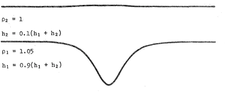
The two layer fluid consists of a lower layer of mean depth h1 and

density pi on a horizontal bottom, and an upper layer of mean depth h2

and density P2 with a free upper su-rface. Attention is confined to fluids

for which the density difference P1 - P2 is small compared with P1 and P2·

The fundamental wavelength is denoted by 2TI.l, and a,b are measure of free

surface and interface wave amplitudes respectively, to be defined more

precisely later. The horizontal and vertical coordinates x,y are

non-dimensional, being measured in uni ts of hi + h2, and the origin of y is on

:),;;

the mean interface, The time t is non-dimensional in uni ts of ( (hi + h2) / g) ",

where g is gravity. Interface displacement, n, and free surface displacement

E;,, are measured in units of b, and both velocity potentials

c/i1,cl>2

in units 3 1:

of ( g( hi + h2) ) 2• The principal small parameter is c

=

b/ ( h 1 + h2) <{ 1, and

other non-dimensional parameters are £'

=

a/ (hi + h2) ~ 1, µ

=

(hi + h2)

I

l b

The governing equations are then

¢ + ¢ _{"' 0} h < y

<

0 (2.la)

lxx lyy

¢ + _<P2yy :: _{0 o < y < 1 h (2.lb)}

2xx

<Ply

·-

0 on y ::: -h, (2.lc)

<Ply nt

s(n<P )

_{lx x} ::::: O(t:2) on y

= o,

(2.ld)

¢2y n, i:; E:(n¢2 ) x x :::::: 0( £2) on y

= o,

(2,le)

+ ~£P ( ¢ 2 + ¢ 2 ) - ~£ ( ¢ 2 + ¢ 2 )

= .

0 ( E 2 ) on y

=

0 '

lx ly 2x 2y

¢ - t;, - £ ( t;,¢ )

=

O( £2) on y

=

1 - h,

'2y t 2x x

¢2t + t;, + st;,¢2yt + ~£(¢22x + ¢2~)

=

0(£2) on y

=

1-h.

Spatially periodic solutions are sought of the form

00

t;, ::;; ~

l

~(t) exp i(k]Jx - wkt) + k=l

00

n

=

~

l

Bk ( t) exp i ( k]Jx - wk t) + k=l

00

*

*

¢1 =~

l

c

1k(t) cosh kµ(y + h) exp i(kJJx -wkt) +

*

k=l

00 ¢2 =~

l

(c

2k(t) cosh k]Jy + D2k(t) sinh kµy) exp :i.(:kµx- wkt) +

k=l

*

(2.lf) (2.lg) (2.lh) (2.2a) (2.2b) (2.2c) (2.2d)

Where 11- denotes complex conjugate, and k, ~ are non-dimensional wavenumber

~ (in units of

1/f)

and frequency (in units of (g/h₁+h 2 )) 2

•

Substitution of these Fourier series in equations (2.1) followed by

neglect of the 0(£) terms yields the linear approximation, whose solution

is (with T 1 = tanh k]Jh T2

=

tanh kµ (1-h))

( P +Ti T2) ( wk2/kµ) 2 - p(T1 +T2) wk2/kµ + (p-1) T1 T2

=

O, ( 2. 3)

Bk

=

(l -T2kµ/wk2) co sh {kp( 1-h)} ~

= (

ikµ/wk) sinh {kµh} elk

(2.4)

·- ( ikµ/wk )D₂k

=

( ikµ/~) (wk 2 /kµ - T2)

I (

1 - T2(u/ /kµ)

c

2k.

Equation

(2.3)

is the dispersion relation, with the solution

(JJ 2

k

kµ

(2.5)

where the larger root will be denoted wAk, and the smaller root wBk. When

p

=

1 + /Jp, /Jp <{ _{1, as in the present application, the two roots reduce to}

w

2 _{= kµ tanh k]J ( 1 + 0 (lip) ) '} Ak

ll]3~

= lip '1'1 T2 /(T1 +T2)(l + O(L:ip)).

The fast wave mode with frequency wAk is the free surface wave mode with

propertj.es almost independent of the presence of the interface. The slow

wave mode with frequency ~k is dependent on the reduced gravity gl\p at the

interface displacement.

The linear solution in equations ( 2. 3) and ( 2. 4) may now be used in

the calculation of the next approximation, that is, in the subs ti tut ion of

equations (2.2) in equations (2.1) including the evaluation of the 0(€)

terms. When the velocity potential amplitudes elk'

c

2k, D2k are eliminated,

two differential equations emerge from lengthy calculation, namely

(with D = d/ dt) ,

D(D-2iU},.)(~+(p-l)(l-Tzkµ/w

₁

/) cosh {kµ(l-h)} Bk)

k-1

--

~

£

.f.~l

Pk,-l

B,e.

Bk-l exp - i(w,e_ +wk-l-wk)t

co

k""l,2, ....• ,

( D - i ( ~ - w Ak wBk

IL\) ) (

D - i (wk + w Ak wBk

I

wk) ) (Bk -(l-'r2kµ/wk2) cosh {kµ(l-h)} Ak)

k-1

-

~

£ )

~

-l B,e, Bk-f exp - i(w.e. + uJk-l - (J.lk)t

.c=l '

k = l , 2 , ...

(2.6a)

(2.6b)

The freq_uencies w_e, defined for positive wavenumbers by equation (2.5)

are continued to negative wavenumbers by

w_.e.

=

-w.e.

(l

>

0). The coefficients

Pk,l , Qk,l are stated in the Appendix. Note that Pk,-l

=

Pk,-(k-l)'

~.-..e.

=

~,-(k-l)'

0

<

..e.

<

k.

Equation ( 2. 6a) has a complementary ftmction which when substituted

into equations (2.2a) or (2.2b) yields wave harmonics with exponents

kµx ± wk t . F'or a given initial displacement, this equation describes

waves of one mode (either fast or slow) propagating in the positive a,nd

negative x-directions, modified as they propagate by the nonlinea.r right

into equations (2.2a) or (2.2b), yields wave modes with exponents

kllx ± wAk wBk/wk t . The frequency wk is equal either to wAk for a fast mode

or wBk for a slow mode. Hence, for a given initial displacement, equation

(2.6b) describes waves of the mode other than that in equation (2.6a)

propagating in the positive and negative x-directions.

If equation (2.6a) is integrated as it stands, the right hand side of

the resulting equation would contain the denominators - i ( W,e + wk-l - wk)

and - i (wk+£. -wt -wk). When all three frequencies in either of these

denominators are of the slow mode, the expressions are 0(µ2) as µ -> 0 interface

(equation 1.1). Since the equations will be applied to long/waves for which

s/µ2

=

0(1), this integration is not permissible. When equation (2.6a) is

multiplied by exp(-2iwk t) , no such difficulty occurs and the equation

integrates to

D(Ak + (p-1)(1 - Tz kµfw/) cosh {kµ(l-h)} Bk)

k-1

-- ~ iE

l

l=l

00

+ i E

l

l=l

+ 0(£2) , k

=

1, 2, ...

When equation (2.6b) is multiplied by the integrating factor

exp - i (wk+ wAk wm/l\.)t and integrated, i t becomes

(D-i(wk-WAk WBk/wk))(Bk-(l-T2 kµ/wk2) cosh {kµ(l-h)} ~)

k-1

= ~ iE

l

l=l

co

+ i E

l

L=l

+ O(t:2) , k

=

1, 2,

If this equation is now multiplied by the integrating factor

(2.7a)

( 2. '7b)

exp ~ i (wk~ wAk luBk/wk) and integrated, the right hand side of the resulting

equation contains the denominators - i ( W,e + wk-l - wAk ~k/wk) and

magnitude small compared with 1 when k and l are such that the triad

describes the near-resonant interaction of equation (1.2). If attention

is restricted to those k and l for which these denominators have a magnitude

comparable with 1, equation ( 2. 7b) may be multiplied by the integrating

factor and integrated to leave

k-1 =-~E:

l

:t=1

00

-€

l

l=l

Benney [ 8] derived equations for the time evolution of long nonlinear

waves, that is, waves for which µ2 "'E: ~ 1. His analysis, applied to the

( 2. 8)

present problem, predicts that for a long nonlinear wave on the free surface

£;, satisfies a Korteweg and de Vries equation, while for a long nonlinear

wave on the interface

n

satisfies a Korteweg and de Vries equation. '.rhe

latter equation is now derived by taking the long wave limits of equations

(2.7a) and

(2.8)

with

wk, W,e_,

U\t-.t

and

wk+i

all referring to the slow

interface wave mode.

The linear long wave velocity on the interface is

Co

=

lim

wBk/kµ,

µ->O

and, from equation (2.3), is the smaller positive root of

Co4 -Co2 +h(l-h)(p-1)/p =

o.

The coefficients

Pk,l/(wk+i-W.e. +wk)

in equation (2.7a) reduce to

Co4 +(3h-2)C0 2

+ l-2h

(1+0(µ2)) Co2 - (1-h)

and the coefficients Q.k,.t in equation (2.8) are 0(µ2) •. On substitution

k-1

= -

~ iEr

l

kµ B,e Bk-l exp - i (w.e. + wk-l

-U\)

t

.e.

=l

00

+ O(E2) , k

=

1, 2, ...

3Co Co4 +(3h-2)Co2 + l-2h

where r

=

-4h (2Co2 -l)(Co2 - (1-h))

(1+0(µ2

) ) .

(2.10)

Equation (2.10) may be summed over

.e.

and k, using equation (2.2b), to give

where, from equation (2.3),

wk/kµ

=

C0 - k2µ2s + 0(µ4),

c

0 ( 1 + ( 3/ p - 2) h ( 1 - h) )

c

0 2 - h ( 1 - h)

and s ""

-6

2

2Co -1

(2.11)

Equation (2.11) is a Korteweg and de Vries equation, as predicted by Benney

[ 8] .

3, Permanent waves on the interface

Permanent periodic waves of (nondimensional) velocity c on the

inter-face have the Fourier expansion

00

n(x,t)::::

l

bk cos kµ(x-ct)

k=l

where from equation (2.2b)

(3.1)

( 3, 2)

When

l\

is eliminated between equations (2.7a) and (2.8), and Bk is replaced

from equation (3.2), then

If the wave height, trough to crest, is denoted by 2b, where

E:

=

b/(h1 +h2), then

00

l

b2k-l

=

-1 k=l

where the origin in x - ct is taken at the trough of the wave.

The properties and method of solution of equations (3.3) have been

described previously

[6]

for permanent waves on a single layer fluid, and ( 3. 4)

apply again here. For waves of length small or comparable with the lesser

of the layer depths, the permanent waves are Stokes' waves on the interface

for which bi

=

-1, bz

=

0( E:). For longer waves, as µ decreases, the nonlinear

interactions between the wave harmonics lie closer to resonance, and the

permanent waves therefore contain more harmonics. Starting from large values

ofµ, equations ( 3.3) may be solved numerically for successively smaller values

of µ to any required numerical accuracy, with the neglect of the 0( E:2)

remainder. One wavelength of the solution for p

=

1.05, h

=

0.9, E:

=

0.05,

and µ = 2 is sketched in figure 1. This periodic permanent wave is closely

approximated by the cnoidal wave solutions of the Kortewel:S and de Vries

equation (2.11), since for a small upper layer (h

=

0.9), the coefficients

rands in equation (2.11) are of comparable magnitude when (l-h)2µ 2 ~ £,

As equations (3.3) are solved for smaller values ofµ at constant p, h~ and£,

the solutions tend towards periodically spaced solitary waves, and the number

of harmonics increases. The solution in figure 1 for µ

=

2 contains 11

harmonics exceeding 10-3 in magnitude, while that forµ=

o.

2 contains '71

harmonics exceeding l0-3 in magnitude.

The present calculations have been checked analytically against two

previous investigations of the long wave limit. Long permanent waves at

the interface of a two layer fluid were investigated by Peters & Stoke:c [

71

~

who developed perturbation expansions for the streamline displacements in the

corresponding steady flow problem. Their solutions agree exactly with the

cnoidal and solitary wave solutions of equation (2.11). Benjamin [9] showed

density and velocity are arbitrary functions of height. When his method is

applied to the particular case of a two layer open fluid, agreement is obtained

again with the cnoidal and solitary wave solutions of equation (2.11).

The coefficient r in equation (2.11) is negative when the interface is

high, positive when the interface is low, and r = O for /J.p ~ 1 when

( 3. 5)

When r

<

0, the cnoidal wave solutions of equation (2.11) are peaked towards

the troughs, as in figure 1. As the upper layer is increased in depth and r

approaches zero, the periodic solutions tend towards the sinusoidal solution

of equation (2.11) for r

= o.

When r

>

O, the cnoidal wave solutions of

equation (2.11) are peaked towards the crests, as in figure 1 inverted. The

same properties are true of the solitary wave solutions of equation ( 2, 11),

although as was noticed 'by Peters and Stoker, there is no solitary wave

solution for which µ 2

₌

0( E:) when r

=

o.

In this case, following Benney [ 8] ,

equation ( 2 .11) may be rewritten

n +Con + 3E2An2

n

+ µ2sn

=

o(s

3

, sµ2, µ4) ,

t x x xxx ( 3. 6)

where )1 - O(s) and A is an 0(1) coefficient, and this equation does have

solitary wave solutions.

4.

Permanent wave structures

Periodic permanent wave structures containing both the fast free surface

wave mode and the slow interface wave mode are now investigated. Solutions

to the governing equations are sought of the form

n

n

=

l

bk cos kµ(x-ct) k=l

m2

~

=

l

~ cos {kµ( x-ct) - at}

k=m₁

(4.la)

where bk ( 1

<

k

<

n), ~ (m1

<

k

<

m2 ) , c and a are to be determinecL The

form of these solutions is such that the interface wave and the envelope

with a constant frequency a relative to the group envelope. The corresponding

complex amplitudes, from equations (2.2)₁ are

Bk(t) = _{bk exp i( wk - kµc)t} 1 <k < n,

~(t)

=

ak exp i( wk - kµc - a)t m1<k <m2.

The significant nonlinear interactions are divided into three types:

( 4.

2a)

(4.2b)

I. Two interface wave modes interacting to modify a third interface wave mode,

1 < ltl, k-t, k <n.

Equation (2.8) is valid for this interaction, since ~,k-l + ~l - u)Ak is

comparable with 1.

( 4.

3a)

II. Two free surface wave modes interacting to modify an interface wave mode,

w - w :!!: w

A,l._+,e

Ai

Bk

( 4.

3b)

Equation (2.8) is valid for this interaction also since wA,k+l -

wAl -

WAk

is comparable with 1.

III. An interface wave mode and a free surface wave mode interacting to

modify a free surface wave mode,

U) o+Wo~WAk

A,k--t.. B{, ( 4. 3c)

Equation (2.8) is valid here also because wA,k-l +

wBl -

wBk is comparable

with 1.

These three types of quadratic interaction dominate all other nonlinear

interactions because of their nearness to resonance. For this reason, they

are the only nonlinear interactions included in the calculations.

The governing equations are formulated in terms of the Fourier amplitudes

defined in equations (

4.

2), for otherwise exponentially large coefficients

are multiplied by exponentially small amplitudes. The free surface amplitudes

Ak (m1 ~ k ~ m2) have associated with them exponentially small interface

amplitudes Bk (m1

<

k

<

m2), so it is possible in principle to use equations

( 2. ~(a), ( 2. 8) throughout the calculations. This is not desfrable in practice

because of the errors caused in the numerical calculations. When equations

equations (4.2), the governing equations become

k-1 n-k

(wBk -kµc)bk

=

~

E .e.I1 (R1)k,-l blbk-l + E .e.I1 (R1)k,l blbk+l

m2-k

+ E

l

(R2)k,l at8k+t l=m1

Min(n,k-mi) ( wAk - kµc - a) ak

=

E

l

l=l

The coefficients RI, R2, R 3 associated with the three types of nonlinear

interaction are defined in the Appendix.

(4.4a)

(4.4b)

Equation (3.4) measuring the height of the interface wave is still valid,

namely

l

bk

=

-1

k odd

(4.5a)

Since the height of the wave group on the free surface is independent of the

height of the interface wave, then

k

~dd

8k

= ;\

1*1ere A is a prescribed constant. The maximum height of the envelope of the

wave group above the mean free surface is denoted by a, where a/(h1 +h2 ) = £1•

It is to be noted that if ~ (m1 .;;;;; k.;;;;; m2) is one solution for the free surface

harmonics, then -ak (m 1 .;;;;; k .;;;;; m2) is another solution with the same envelope.

The n+m2-m1+3 equations (4.4), (4.5) are now solved for the n+m2-~m1+3

variables bk (l .;;;;;k .;;;;;n), 8k (m1 .;;;;;k .;;;;;m2), c and a.

_5_. __ R_ermanent wave structures of short wavelength.

The simpler solutions of equations (4.4) and

(4.5)

include those of short

wavelength, when the wave on the interface is almost sinusoidal because the

first type of interaction is far from resonance. For a free surface wave

group of sufficiently small amplitude, equations (4.4a), (lt.5a) are then

(5.1)

This set of m2 - m1 + 1 linear algebraic equations has in general m2 - m1 + 1 sets

of solutions, each set containing an eigenvalue a and the corresponding

eigenvector~ (m1 < k <m2) of the matrix of coefficients. Each eigenvector

may be scaled to satisfy equation (4.5b).

It is a straightforward numerical calculation [10] to find the eigenvalues

and eigenvectors of the set of equations (5.1) for any given external parameters.

These parameters were taken to be p

=

1.05, h

=

0.9, µ

=

20, £

=

£1

=

_0.005,

for which the equality ~l

=

dwAk/dk occurs at about k

=

l0.5. The interval

m1 ~k <m2 was chosen to be sufficiently large that sets of solutions were

reproducible to within the desired numerical accuracy (10-4) when the size o:f

the interval was increased further. Each set of solutions was then used as

the starting estimate for a Newton-Raphson solution of equations (4.4) and

( 4. 5) to the same numerical accuracy. The first five sets of solutions are

drawn in figure 2( a), and the corresponding free surface wave groups (equation

4.1b) a.re drawn in figure 2(b).

In order to understand the sets of solutions in figure 2(a), equations

(5.1) are written as the set of difference equations

where (R3\,-l ~ (R3)k',₁ , and f(k) is approximately a quadratic form in

A comparison of these difference equations with the differential equation

d2

~

+ f(x)y

=

0 ,

-~ k.

(5.2)

shows that solutions for ak are oscillatory in k when f(k)

>

O, and are

convergent or divergent in k when f(k)

<

O. The only stationary value of f( k)

k · t · d ( k ) th t · ,,,.

I

1

ma es 1 a maximum near dk wAk - wBl - a = 0, a is, near wBl "' Ul.!lAk

a

L Hence acceptable solutions for ak (m1 < k < m2) consist of' a range in the

neighbourhood of resonance where ak is an oscillatory function of k 9 enclosed

by ranges at each end where ak decreases monotonically in magnitude towards

of the range of oscillation and the number of oscillations of ak as a function

of k both increase when a decreases. These properties are all present in the

five solutions sketched in figure 2(a).

The structures of the free surface wave groups in figure 2(b) may be

interpreted in terms of their interaction with the horizontal velocity field

caused at the free surface by the wave on the interface. Since the wave on

the interface is sinusoidal, the horizontal velocity u at the free surface is

also sinusoidal with a positive maximum at the centre of the group and a

negative minimum at the two ends of the group. The resonance equation (1.2)

is modified now to

( 5. 3)

where c

=

0.035 and -0.001::;;; u e;;;; 0.001 (from equations 2.2d, 2.4) for the wave

groups in figure 2(b). Hence the wavenumber of the free surface wave within

the group varies from 10.8 at the centre of the group to

9.6

where the group

extends to the ends of the fundamental wavelength. Measurements in figure 2(b)

confirm the accuracy of this interpretation.

6.

Permanent wave structures of long wavelength.

When the fundamental wavelength increases, the first type of interaction,

namely that 'between harmonics on the interface, moves closer to resonance.

The number of interface harmonics therefore increases, and since each interface

harmonic interacts near resonance with a range of pairs of free surface

harmonics, the number of free surface harmonics also increases. 'l~e latter

effect may be seen alternatively as a consequence of a longer interface wave

causing a stronger horizontal velocity gradient at the free surface.

Two methods have been developed for calculating numerically the solutions

of equations

(4.4), (4.5)

for long wavelengths. The harmonics of a permanent

interface wave of given wavelength in the absence of a free surface wave group,

bk ( 1

<

k e;;;; n) , may be calculated as in § 3 and then substituted into eque,tions

(tr.4b). 'l~e resulting linear algebraic equations for ak (m1 ~k ~m2) and a

and the solution used as a starting estimate for a Newton-Raphson solution

of equations (4.4), (4.5) at the given wavelength. Alternatively, the

solutions in

§5

at short wavelengths may be continued step by step inµ to

long wavelengths, using the Newton-Raphson method of solution at each step.

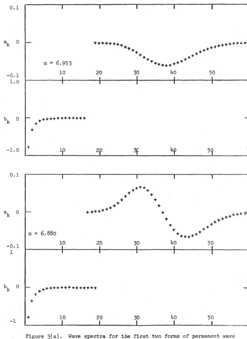
The first two sets of solutions for the harmonics at p

=

1.05, h =0.9,

µ

=

2, £

=

£1

=

_{0.01 are shown in figure 3(a), and the corresponding}

permanent wave structures are sketched in figure 3(b). It can be seen that

the shape of the spectra of the free surface harmonics in figure 3(a) is the

same as that of the first two fo:i;-ms in figure 2( a). This similarity of shape

was found for all five forms in figure 2(a) as µ decreased from 20 to 2. The

free surface wave groups in all five forms of permanent wave structure also

retained similarity of shape as µ decreased.

The horizontal velocity at the centre of the free surface wave group is

0.008, 0.009 respectively in the two examples in figure 3(b), and the phase

velocity is 0.066, 0.067 respectively. Equation (5.3) therefore predicts that

the wavenumber at the centre of the free surface group should be about 37

in both examples. The validity of this interpretation is confirmed by figure

3( a), where k

=

37 lies near the centre of the spectrum in both examples, and

by figure 3(b), where measurement of the wavelength within the free surface

wave group agrees with this estimate.

The interface wave spectrum is broader in the presence of a wave group

than in its absence. The interface spectrum for the first form of permanent

wave structure in figure 3 contains 15 harmonics exceeding 10-3 _{in magnitude,}

while the interface permanent wave spectrum in the absence of a surface wave

group contains only

6

harmonics exceeding 10-3 in magnitude. The free surface

wave group, through the second type of nonlinear interaction identified in §4,

broadens the interface wave spectrum and hence sharpens the interface wave,

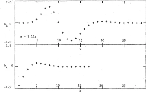
The amplitude of the free surface wave group (measured by £ 1) may be

increased step by step so that the second type of nonlinear interaction causes

a greater change to the shape of the wave on the interface. One such example

structure at p

=

l.05, h

=

0.9, µ

=

2, e: = 0.01, e:'

=

0.05.

The spectrum of the free surface harmonics in figure 4(a) displays the

characteristic shape of the second form of permanent wave structure, but the

spectrum of the interface harmonics, instead of decreasing monotonically in

magnitude as previously, now displays a small overshoot. It can be seen in

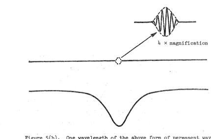
figure 4(b) that the shape of the envelope of the free surface wave group has

been impressed onto the interface wave, which is a property that also occurs

for the other forms of permanent wave structure in this limit. The phase

velocity of the structure has increased from 0.067 at e:

=

e:'

=

0.01 to

0.124 at e:

=

0.01, e:'

=

0.05 because the structure is now dominated by the

fast free surface wave mode. The horizontal velocity at the centre of the

free surface wave group due to the interface wave is now 0.010, so equation

( 5.

3) predicts that the wavenumber at the centre of the free surface wave

group should be about 10. This is in agreement with figures 4(a) and 4(b).

The wavenumber is smaller than in the examples of figure 3 because the phase

velocity of the structure is larger, requiring from equation (5.3) a larger

free surface group velocity.

The amplitude of the interface wave (measured by e:) in the examples of

figure 3 may be increased step by step while the amplitude of the free surface

wave group is held constant. Figure 5 shows the first form of permanent wave

structure at p

=

1.05, h = 0.9, p

=

2, e:

=

0.05, e:'

=

0.01. The phase velocity

of the structure is

o.

074, which is the same (to this accuracy) as the phase

velocity of the permanent interface wave in the absence of a free surface wave

group. 1_{.rhe horizontal velocity at the centre of the free surface wave group}

due to the interface wave is 0.045, and from equation (5.3) the wavenumber at

the centre of the free surface wave group is therefore about 150. This is

consistent with figures 5(a) and 5(b). The central wavenumber is much larger

than in the examples of figure 3 because the horizontal velocity at the free

surface is much larger, requiring a smaller group velocity in equation (5.3).

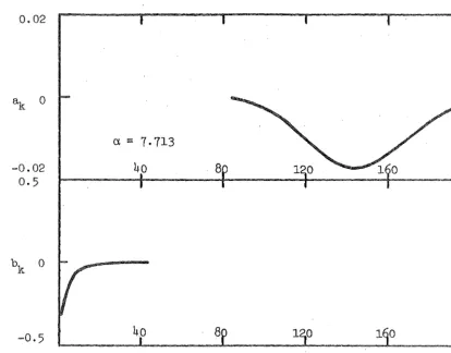
When the fundamental wavelength is increased while all other parameters

of solitary permanent wave structures. ·.fue central quarter of one wavelength

of the first form of permanent wave structure at P

=

1.05, h

=

0.9, µ

=

0.5,

£

=

£1

=

_{0.01 is drawn in figure 6(b). The remainder of the wavelength consists}

of a level free surface and a level interface. The spectra of harmonics of the

interface and free surface waves are drawn in figure 6(a) as continuous curves

for convenience and because they approximate to the Fourier transforms of a

solitary permanent wave structure.

In all the calculations above, the depth of the lower layer is fixed at

0.9 of the total depth (h

=

0.9). As this ratio is decreased with all other

parameters held constant, the horizontal velocity field at the free surface

due to the interface wave also decreases, since the interface moves further

from the free surface. Beginning from the example of figure 3, as h is

decreased at constant p, µ, £, and E1

, the spectra of the interface wave and

free surface wave tend towards those of the example in figure 2. The number

of harmonics in the interface wave decreases as h decreases until about

h

=

0.35, when the second harmonic passes through zero. When his decreased

further, the number of harmonics in the interface wave increases again, but

the number of harmonics in the free surface wave remains small because the

horizontal velocity field at the free surface is also small.

7.

Discussion

The permanent wave structures described here consist of a wave of permanent

shape at the interface and a wave group of permanent envelope at the free

surface. An interface wave has permanent shape when the linear dispersion and

the nonlinear steepening or flattening of inclined surfaces is in balance

([9],

§1). There is a similar explanation for the permanent shape of the free

surface wave envelope. The horizontal velocity field at the free surface due

to the interface wave has a forward maximum above the wave trough, decreasing

on either side of the trough. Hence a free surface wave behind the trough is

stretched and therefore moves faster, since the phase velocity is an increasing

is compressed and therefore moves slower. The net effect for the free

surface waves is one of balance between the linear dispersion and the nonlinear

interaction with the interface wave.

This physical argument mEcy" be applied also to wave groups of permanent

envelope on deep water ([11), §17.8). In this case, there is a balance between

linear dispersion and the mean quadratic velocity field caused at the free

surface by the wave group itself.

On comparing the different forms of permanent wave structure in figures

2 or 3, for example, it can be seen that the higher the form, the more complex

is the shape of the free surface wave group, although the interface wave

remains almost unchanged. Hence, when all other parameters are held constant,

the energy of the permanent wave structure is expected to be greater, the higher

the form of structure. This in turn implies that the higher forms are less

stable, and that the first form of permanent wave structure is most likely

to occur in practice. A stability analysis will be made to test this argument.

The unsteady solutions of equations (2.7) will also be investigated. The

second type of nonlinear interaction identified in

§4,

for example, generates

interface waves whenever there is a spectrum of free surface waves. When the

free surface waves are forced by the wind, this interaction provides a

near-resonant mechanism for the generation and growth of interface waves. The

permanent wave structures described here may in some sense represent an

asymptotic state for waves on a two layer fluid.

Acknowledgment.

The author is grateful to Professor David J, Benney for suggesting this

References

1. D.J. Benney Significant interactions between small and large scale

surface waves. Stud. AppZ. Math. 66, 93-106 (1976).

2. M.S. Longuet-Higgins

&

R.W. Stewart Changes in the form of short

gravity waves on long waves and tidal currents.

J.

FZuid Meah. 8, 565-583 ( 1960).

3, A.E. Gargett

&

B.A. Hughes On the interaction of surface and internal

waves. J. FZuidMeah.

62,

179-191 (1972).

4.

John E. Lewis, Bruce M. Lake

&

Denny R.S. Ko On the interaction of

internal waves and surface gravity waves. J. FZuid Me ah. 6 3 , 773-800 ( 1974).

5. P. J. Bryant Periodic waves in shallow water. 'J. FZuid Meah. 6 9 , 625-644 (1973).

6.

P.J. Bryant Stability of periodic waves in shallow water.

J.

FZuid Me ah. 6 6 , 81-96 ( 1974) •

7. A.S. Peters

&

J,J, Stoker Solitary waves in liquids having non-constant

density. Comm. PU!'e AppZ. Math.

13,

115-164 (1960).

8. D.J. Benney Long non-linear waves· in fluid flows. J, Math & Phys. 4 5 ~ 52-63 ( 1966) •

9. T.B. Benjamin Internal waves of finite amplitude and permanent form.

J. FZuid Me ah.

2

6 , 241-270 ( 1966) •

Appendix.

Define Fk

=

~ cosh µk(l-h) -µk sinh µk(l-h),

Gk

=

w~ sinh µk(l-h) - µk cosh µk(l-h).

Then

Pk

,.t

=

l@k [( P-1 )(

w} - w

.t"'k+l + <{+,el

p(

~+l

-

w

l) [ wk+l .

w

l

l

- + _ __.,;;.._

tanh µkh tanh µ(k+l)h tahh µlh

PW.e_ ~+l

2 2

Wo Wk+o [ U2 £(k+.f.)

+ .c.. .c..

w

2 (

w

2 -

w

w

+

w

2

-2F p Flr+P. k

l

l

k+l k+l

W.e_

Wk+l

2 k+l l ]

- (~+£. - w.ehJ k(-w- +

w ) ;

k+l

l

_ µ2 k2 tanh µkh tanh µk(l-h)

~,l

-

2w~(

p + tanh µkh tanh µk( 1-h))

p(wk+l - wl) [

~+£.

+

tanh µkh . tanh µ(k+l)h

- tanh µlh tanh µ(k+l)h +

+ ( ) ( p - (

P-:p

µk ) (

w

Gk+l +

w

o GFl )

(Both

(R2)k,l

and

(Rs)k,l

may be approximated by simpler expressions

P2

=

1

pl = 1.

05

[image:24.598.173.554.369.531.2]

h1

=

o.9(h1 + h2)

I .)' I .)' I

.

.,,/"'

i !lJ I

:J'

0 0 0 00 00 :>;' 00

.

.

.

.

!\) !\) I\) I\) I\) !\) I\) I\) I\) \J1 0 \J'l \J1 0 \J1 \J1 0 \J1 \J1 0 \J1 \J1 0 Q + Q Q Q Q Ii

•

II I! II II I\) + !\) + I\) +

+

•

I I I\)

•

I\) 0 I-' I-' I-' I-'

.

+

.

+

.

+

.

t

.

t

\() I I-' I

s;

)

w w \.nl-\() + V1 I-' \ \J1 \J1 I-' \J1 ·co + \J1

I

I-' . -..;i I-'

•

~·

+'

\"

+

.J

L

+·

"+

..

~

+---~

...

,

r+/

+ b~

.,,,..-ci++~

b

-,

b

~~

/

----1,

~--~+

.

:>;'j ~' :>;'I :>;' :>;' .. , :>;'

..

,

..

--

·--..

~

..

,

'+'

+'

..

,

+.

1-'j--t:/

I-'

'·

I-' I-'

'+

I-'

\

\J1 ' \J1

'·

\J1

..

,

\J1 \ \J1

.,

'

\

'

t

.,

t

+ + \

i

•

...

+ +

1

\

'

I + + ~~

1

I\) I I\)

i

!\)

•

I\)

t

0

1

0 0 + 0 +

I

..

Figure

( _{=l 0}

=l

I _{=l 0}

=l

I _{:::l 0}

=l

I _:::l

=l

I =l _{0 :::l}

0.1

0

-0 .. 1

1. 0

-1.0

0.1

0

-0.1

1

-1

a= 6.953

10'

++++++++++++++

1

20

2

a

=

6.880

+ +

10 20

+++++++++++++++

+

10 20

30

40

50

3

4

5

30

4o

50

30

40

50

Figure 3(a). Wave spectra for the first two: forms of permanent wave

[image:27.600.57.538.83.742.2]

..r1'M1l''i.,,

---V,JL/\l(.Y'~---Figure 3(b). One wavelength of the first two forms of permanent wave

structure at long wavelength with E

=

E1

=

0.01 (vertical magnification

I. 0

-1. 0

1. 5

...:i.5 +

a.

=

7.ll.L 5

•

• +

10

•

• • • 15

k

•

+ • • •

• + • • +

+ • • • •

1 1

k

• • • • • • • • • ~ + ~

20

25

2 2

Figure 4(a). Wave ~pectra for the second form of permanent wave structure

at long wavelength with

e:

=

0.01,

e:'

=

0.05.

Figure 4(b). One wavelength of the above form of ;r:iermanent wave structure

[image:29.600.45.532.107.424.2] [image:29.600.82.537.395.793.2]

0.005

-0.005

1.0

-1.0

a

=

30.901

40

Bo

4o

80

120 160

Figure 5(a). Wave spectra for the first form of permanent

wave structure at long wavelength with 8

=

0.05, €1

=

0.01.

The discrete points have been replaced by a continuous curve.

p '

Figure 5(b). One wavelength of the above form of permanent wave

[image:30.602.98.521.83.403.2] [image:30.602.91.521.509.793.2]

0.02

0

-0.02

0.5

ct=

7.713

4o

4.o

8

8 1 0 1 0

Figure 6(a). Wave spectra for the first form of permanent

wave structure at very long wavelength.

•/

The discrete points·have been replaced by a continuous curve.

Figure 6(b). The central quarter of one wavelength of the above

[image:31.621.84.515.90.727.2] [image:31.621.97.511.99.423.2]