Analysis of Machine Learning Techniques Applied to the
Classification of Masses and Microcalcification Clusters in
Breast Cancer Computer-Aided Detection
Edén A. Alanís-Reyes, José L. Hernández-Cruz, Jesús S. Cepeda, Camila Castro, Hugo Terashima-Marín, Santiago E. Conant-Pablos
Evolutionary Computation Research Chair, Instituto Tecnológico y de Estudios Superiores de Monterrey, Monterrey, México. Email: [email protected]
Received September 1st, 2012; revised October 4th, 2012; accepted October 15th, 2012
ABSTRACT
Breast cancer is one of the most common and deadliest types of cancer among women and early detection is of major importance to decrease mortality rates. Microcalcification clusters and masses are two major indicators of malignancy in the early stages of this disease, when mammography is typically used as the screening technology. Computer-Aided Diagnosis (CAD) systems can support the radiologists’ work, by performing a double-reading process, which provides a second opinion that the physician can take into account in the detection process. This paper presents a CAD model based on computer vision procedures for locating suspicious regions that are later analyzed by artificial neural networks, support vector machines and linear discriminant analysis, to classify them into benign or malignant, based on a set of features that are extracted from lesions to characterize their visual content. A genetic algorithm is used to find the subset of features that provide the greatest discriminant power. Our results show that the SVM presented the highest overall accuracy and specificity for classifying microcalcification clusters, while the NN outperformed the rest for mass-classi- fication in the same parameters. Overall accuracy, sensitivity and specificity were measured.
Keywords: Computer-Aided Diagnosis; Breast Cancer Detection; Breast Cancer Diagnosis; Mass-Segmentation;
Calcification Segmentation; Digital Mammography
1. Introduction
Breast cancer is one of the most common and deadliest types of cancer among women in the world. It is reported that this disease is found in 25 of every 100,000 persons, of which 99% are women [1]. Early diagnosis and effec- tive medical treatment are the only options we have to decrease mortality rates, since there is no way to effec- tively prevent this disease. Consequently, women should undergo breast exams in a regular basis, which can in- clude physical exams, mammograms, ultrasonography, among others. However, out of all the available exams, screening mammograms are the best tool when it comes to early diagnosis of breast cancer because they can de- tect lesions even before they become palpable. A suc- cessful detection of this disease in its earliest stages is a key point for patient survival, since it brings the opportu- nity to follow the appropriate medical treatment to cure this affection [2].
A mammography is a non-invasive screening tool, recommended for young women who have symptoms of breast cancer or have a high risk of breast cancer, given
their family history, as well as for women older than 40 even if they have no signs of the disease. Breast cancer lesions that mammography may reveal include calcifica- tions, masses, architectural distortions and asymmetric densities.
Breast cancer screening by way of mammography provides a sensitivity of 79% and a specificity of 90% [3], and is often complemented with other clinical studies that include biopsy, which has a very high specificity, or even a second diagnosis performed by a different radi-ologist, which is a redundant process that increases sen-sitivity in 15% [4].
Therefore, several research efforts have been directed towards the design and development of Computer-Aided Diagnosis (CAD) tools, often based on artificial intelli- gence techniques, which can support the radiologists’ work, by performing a separate analysis which provides a second opinion that the physician can take into account.
design and develop a CAD system that can be able to automatically detect and diagnose breast cancer lesions in early stages.
Our work describes an implementation of a CAD sys- tem that analyzes digital mammograms to detect and classify microcalcification clusters and masses, which are known to be the two major indicators of malignancy as stated in [7]. We use computer vision techniques for the detection of suspicious areas that may contain the afore- mentioned lesions and, afterwards, we use three AI-based classification methods to assess their malignancy, namely: artificial neural networks, support vector machines and linear discriminant analysis.
This document begins with a description of several re- lated works. Then we present the methods and materials which we used to develop our research, describing the stages considered within our CAD and the implemented procedures, from preprocessing the input image from the classification of the lesions that were found. Finally, the experimentation phase is described and the assessment of performance of the considered classifiers is presented in the results.
2. Related Work
Breast lesions have a wide range of features that can in- dicate malignancy. However, not all changes in breast tissue are malignant; they could be benign and some- times cannot be distinguished from the surrounding tis- sue, which makes the detection and diagnosis process even more difficult for physicians. In fact, it is reported that 65% to 90% of the biopsies of suspicious lesions turn out to be benign [10], as a result of medical misin- termpretation of some cases that finally lead to a large number of false positives.
Hence, it is of major importance to develop methods capable of increasing the lesion-detection and cancer- diagnosis accuracy, for physicians to make better deci- sions regarding an appropriate follow-up and biopsy. One powerful option is the use of computers in process- ing and analyzing biomedical images, such as mammo- grams, since they provide the radiologist with relevant information, which may not be readily observed by the physician, resulting in an enhanced detection/diagnosis process.
An important step in a CAD system is the segmenta-tion of the image to detect the lesions. In [11], authors considered regions determined by binarized images to segment lesions at multiple threshold levels. Their me- thod achieved a sensitivity of 80% and 2.3 false-positives per image. Another study [12] proposed a methodology for estimating the probability of each pixel in an image as being part of a lesion, based on the concept of using Gaussian mixture models.
Once the segmentation phase has found suspicious re- gions of interest (ROI) containing abnormalities, a fea- ture extraction phase is performed. In [13] authors ana- lyzed the performance of temporal features as detector of masses, implementing a pixel-level algorithm; in each ROI, they extracted 20 texture features, 3 spiculation features and 12 morphological features. The study re- mported in [14] claimed that entropy, standard deviation and the number of pixels is the best feature set to distin- guish a benign microcalcification pattern from a malig- nant one. They took into account 14 features, which were combined and analyzed with a neural network, in order to find out what was the most appropriate combination.
As one can see there are several mammographic fea- tures that can be taken into account for classifying le- sions, and it is important to know which subset of them provides the highest discriminant power to determine which lesions are benign and which malignant.
To achieve this goal, once a set of features has been computed, they should go through a feature selection step, in which several techniques have been explored. In [9] authors present a method called PSO-kNN based on Particle Swarm Optimization (PSO), that serves to select parameters in an heuristic way and uses a k-nearest neighbor (kNN) technique method for classification of lesions. The study presented in [15], compared a genetic algorithm (GA) approach for selecting the most relevant features extracted from both individual microcalcifica- tions and microcalcification clusters (MCC), against the methods used in [16,17], where features are ordered ac- cording to their class separability.
The final step, after the subset of most discriminant features has been computed, is to classify lesions into benign or malignant. Several techniques have been ex- plored in this stage, including Support Vector Machines (SVM), Artificial Neural Networks (ANNs), Evolution- ary Artificial Neural Networks (EANNs), among others. An approach to classify mammographic masses as ma- lignant or benign, by using interval change information was presented in [18]. In [19], authors proposed a pro- cedure for the classification of MCCs in mammograms using three EANNs. Moreover, EANNs have also been applied in different classification tasks like in [20]. Au- thors in [8] proposed a SVM-based approach to distin- guish microcalcifications from other ROIs. A study on the performance of several classifiers is presented in [6], including SVM, ANN, Bayesian and kNN techniques.
An extensive survey of related literature can be found in [5].
3. Methods and Materials
masses in digital mammograms that are fed as input, and the assessment of their malignancy. As an output, the system provides an image with overlaid marks in the regions where lesions where found, and an indication of whether the lesion is considered benign or malignant.
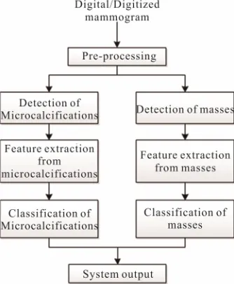
Figure 1 depicts the overall design of our CAD system.
The first stage implements a pre-processing mechanism, which has the objective of eliminating the elements in the mammographic image that could negatively affect the subsequent processes of detecting potential lesions, both calcifications and masses. Those detection processes are performed separately and once the lesions are segmented and extracted as ROIs, a set of features are computed in order to characterize their visual content. Then, using a GA, our system determines the subset of features that provides the highest classification performance, which is finally used in the classification step to determine whe- ther the detected lesion is considered a malignant case or not.
An insight of the inner workings of each phase in our CAD system is provided in the following sections.
3.1. Pre-Processing
Mammograms often present noise and artifacts that were acquired during the creation of the x-ray image and/or during the digitization of a hard mammography, due to changes in illumination and distortions in the properties of the digitized image. Besides, the background of a typical mammogram contains labels and marks that are not useful for the analysis of breast cancer itself; and therefore have to be removed, to prevent the subsequent stages from being negatively affected.
This pre-processing method takes the original mam-
Figure 1. Proposed CAD system.
[image:3.595.307.539.433.686.2]mography as input and applies a median filter to elimi- nate noise located in the background, while keeping im- portant features of the image, like the breast tissue. In this process, a 3 × 3 mask was used, centered in each pixel within the image, and the value of that pixel was replaced by the median of the surrounding mask pixels. The size of this mask was chosen empirically, trying to avoid the loss of local details, as described in [15]. Fur- thermore, the background marks and the isolated regions are deleted, for the image to contain only the breast tissue, by way of a binarization process in which all pixels that are not within the group of those corresponding to the breast are removed. The complete process is depicted in
Figure 2.
3.2. Detection of Lesions
As depicted in Figure 1, once the image has been pre-
processed, the next steps are the automatic detection of microcalcifications and masses.
Figure 3 describes the stages related to the process of
detecting clusters of microcalcifications, applied to a representative case, shown in Figure 3(a). The first step
is to highlight microcalcifications, by way of contrast adjustment, followed by a negative filter and, lastly, a mean filter with a 2-pixel window since calcifications are usually represented by small regions.
Next, the resulting image is used to find the edges of
(a) (b)
[image:3.595.89.256.514.717.2](c) (d)
microcalcifications, by applying an edge detector based on a Difference of Gaussian (DoG) filter with a 26-pixel window and a theta value of 0.363. The resulting image is shown in Figure 3(b). Then, we execute a Gaussian
Blur filter with a 3-pixel window and a theta value of 4.8 to smooth the image for further processing.
The third step consists in binarizing the image, using a gray-scale threshold that narrows the complete scale (0 - 255) to a more representative 25 - 230 scale, resulting in the image shown Figure 3(c). Finally, we use the
bi-narized image as a mask to segment the original image and extract the regions of interest, providing the image presented in Figure 3(d) as a result.
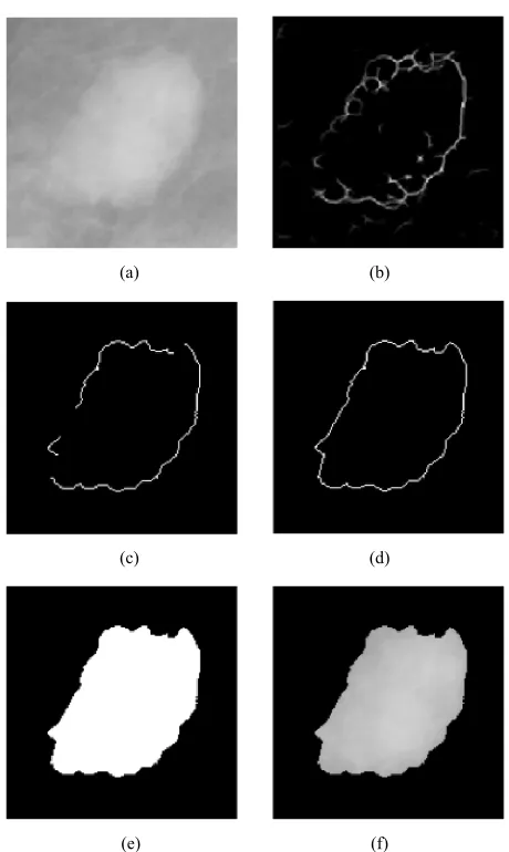
On the other hand, the detection and segmentation of masses was performed by using seven procedures: loca- tion of masses using an adaptive global threshold, edge detection, region growing edges, elimination of overlaps, union of edges, internal binarization and segmentation.
Figure 4 illustrates the stages of this process.
In order to determine the location of suspicious masses, we use a global adaptive threshold segmentation process, which analyzes the global information of the image based on its histogram and determines an appropriate threshold to segment different areas [21]. At this point the masses have been located in the image and the fol- lowing procedures will focus only on those regions con- taining masses.
Once the masses have been located, we proceed to de- tect its edges, in order to determine its shape and contour, with the objective of obtaining necessary information for the following phases. The technique used for this purpose is edge detection based on wavelet transform. This edge detection algorithm accumulates the multiscale-wavelet edges and generates an image with some points that do not necessarily represent the margin, as depicted in Fig- ure 4(b). Thus, a refinement process should be con-
ducted.
Consequently, in order to refine the line of the margin of the mass, we use a region-growing edge technique, that starts from some seed points and it continues by adding representative pixels iteratively verifying the nei- ghbors of pixels that meet certain criteria [22]. Figure 4(c) shows the resulting image up to this point.
Once the edges of the masses have been identified, we perform a process aimed to connect the edges that were found. This union process draws straight lines from the end of one edge to the start of its nearest one, as depicted in Figure 4(d).
Once we got a continuous line as the border of the mass we run the binarization process, which results in the image presented in Figure 4(e). The purpose of the
bi-narization of the internal region surrounded by the edge is to have a binary image that will serve as a mask for
cutting the area comprising the mass in the original im- age. Finally, the segmentation procedure extracts the area corresponding to the mass to perform subsequent calcu- lations over this area, as depicted in Figure 4(f).
3.3. Feature Extraction
Once the lesions were detected and extracted as ROIs, they are used to compute a set of features that describe their visual content, with the objective of enabling a clas-sification algorithm to discriminate between benign and malignant cases.
Having detected all individual calcifications in one image, an algorithm for locating regions where density (the amount of them per cm2) is higher was performed, in order to detect so-called clusters of microcalcifications. For this, all pairs of individual microcalcifications within a Euclidean distance less than an empirically defined threshold of 100 pixels are regarded to be a subset of neighboring microcalcifications; these subsets are ex- plored to find the one with the highest density and select it as a new cluster. The process is then repeated with the remaining ungrouped microcalcifications until all are included in a labeled cluster.
Afterwards, all detected clusters are passed on to the feature extraction process, in which 30 features, listed in
Table 1, are computed from them. There are 14 features
which define the shape of a cluster, 6 which describe the area of the individual microcalcifications and 10 for the
(a) (b)
(c) (d)
(a) (b)
(c) (d)
(e) (f)
Figure 4. Steps of the mass detection stage. (a) Pre-processed image with a mass; (b) Detected borders; (c) Growing edge process; (d) Connection of edges; (e) Binarized image; (f) Segmented mass.
absolute contrast between the calcifications and their background, as described in our previous work reported in [15].
Also, once all masses have been detected in a mam- mogram, they are passed on to the feature extraction process, in which 50 features are computed from them. The complete list of features for masses is shown in Ta- ble 2. There are 7 features that describe the signal con-
trast, 7 features that define background contrast, 3 fea- tures for representing the relative contrast of the image and 20 features for shape. There also are 6 features for contour sequence moments and 7 features that describe the first invariant moments.
[image:5.595.57.287.90.475.2]Once the features for each ROI have been extracted, the whole set goes through a feature selection process that will result in a subset of them that provides the highest performance for a given classifier, with a reduced
Table 1. Features extracted from microcalcification clusters.
Computed Features
Clustershape (14 features)
Number of calcifications, convex perimeter, convex area, compactness, microcalcification density, total radius, maximum radius, minimum radius, mean radius, standard deviation of radii, maximum diameter, minimum diameter, mean of the distances between microcalcifications, standard deviation of the distances between microcalcifications.
Area of microcalcifications
(6 features)
Total area of microcalcifications, mean area of microcalcifications, standard deviation of the area of microcalcifications, maximum area of the microcalcifications, minimum area of the microcalcifications, relative area.
Microcalcification contrast (10 features)
Total gray mean level of microcalcifications, mean of the mean gray levels of
microcalcifications, standard deviation of the mean gray levels of microcalcifications, maximum mean gray level of
[image:5.595.311.539.117.441.2]microcalcifications, minimum mean gray level of microcalcifications, total absolute contrast, mean absolute contrast, standard deviation of the absolute contrast, maximum absolute contrast, minimum absolute contrast.
Table 2. Features extracted from masses.
Computed Features
Signal contrast (7 features)
Maximum gray level, Minimum gray level, Median gray level, Mean gray level, Standard deviation of the gray level, Gray level asymmetry (skewness), Kurtosis of gray level.
Background contrast (7 features)
Maximum gray level, Minimum gray level, Median gray level, Mean gray level, Standard deviation of the gray level, Gray level asymmetry (skewness), Kurtosis of gray level.
Relative contrast (3 features)
Absolute contrast, Relative contrast, Portional contrast.
Shape (20 features)
Area, convex area, background area, filled area, perimeter, maximum diameter, minimum diameter, orientation, eccentricity, Euler number, circular diameter equivalent, solidity, Extent, shape factor, roundness, aspect ratio, enlongation, compactness 1, compactness 2, compactness 3.
Contour sequence moment (6 features)
Contour sequence moment 1, contour sequence moment 2, contour sequence moment 3, contour sequence moment 4, mean radii, standard deviation of radii.
First invariant moments (7 features)
dimensionality of the dataset. For this process we im- plemented a wrapper approach that considers a GA to analyze the performance of three different classifiers, namely: a feed-forward back-propagation neural network (NN) [23], a Support Vector Machine (SVM) classifier [24] and a Linear Discriminant Analysis (LDA) method [25,26]. This feature selection process was carried out separately for clusters of microcalcifications and masses.
The chromosomes of the individuals in the GA contain an amount of bits equal to the total number of features, i.e. one bit for each extracted feature. The value of the bit determines whether that feature will be selected or not and consequently if it will be considered in the subset of features that will serve as an input to the classifier. Thus, each individual is evaluated by constructing, training and testing a given classifier algorithm and reporting the overall accuracy of the model as the fitness of the indi- vidual.
The GA can stop due to two reasons: either the gen- erations limit has been reached or no improvement on the evaluation of the best individual has been observed dur- ing five consecutive generations. Afterwards, the classi- fier with the best performance is obtained along with the subset of features that have the highest discriminant power.
3.4. Classification of Lesions
Once we have performed the feature selection process and, found the subset of features that are more relevant for the classification task, it is necessary to assess the performance of the aforementioned classifiers of interest. This analysis is performed separately for microcalcifica- tion clusters and masses. Consequently, with this test we can determine which is the best classification approach for each one of those lesions, independently.
In this stage a 10-fold crossvalidation scheme is per- formed, in which the accuracy, sensitivity and specificity of each classifier was measured. The dataset of features of lesions and the corresponding diagnosis was divided into ten non-overlapping splits, considering 9 of them (90% of the data) for training and the remaining split (10% of the dataset) for testing. The process was re- peated ten times, each one using a different split on the data for testing.
4. Experiments and Results
The mammographic database used in this research work was provided by the Mammographic Image Analysis Society (MIAS) [27]. All experiments were performed in MATLAB Version 7.8.0.347 (R2009a), under a 2.8 GHz Intel Xeon processor with 3.48 GB of memory.
For the process of selecting features from clusters of
microcalcifications and masses, we used a wrapper me- thod with a GA. In the case of microcalcification clusters, the GA contained individuals with chromosomes of 30 bits of length, representing the inclusion (or exclusion) of each one of the 30 features extracted from the clusters. For mass-related features, individuals had a length of 50 bits.
In both cases, a simple GA was used, with a popula- tion of 50 individuals, binary tournament selection, two- point crossover and fitness based reinsertion. The prob- ability of crossover was set to pc = 0.7 for cluster-features
and pc = 0.9 for mass-features; the probability of
muta-tion was pm = 0.1 in both processes. The initial
popula-tion of the GA was initialized uniformly at random and ran for 50 generations.
This feature selection process was replicated sepa- rately for clusters and masses. In both executions, the process was performed three times, one for each of the classifiers of interest (NN, SVM, LDA).
The NN had a single neuron in the output layer and complying with Kolmogorov’s theorem [28], one hidden layer with 2n + 1 neurons, where n is the number of input units. All neurons had the sigmoid hyperbolic tangent as transfer function. The data (inputs and targets) were scaled in the range [−1, 1] and divided into ten non- overlapping splits, containing 90% of the data for train- ing and 10% for testing. As for the SVM, we used the Gaussian Radial Basis Function kernel, with a scaling factor of σ = 2.0 and the Quadratic Programming tech- nique to find the separating hyperplane. Finally, we also considered the Linear Discriminant Analysis method to construct as the third classifier.
5. Results for Clusters of Calcifications
Table 3 shows the results of the feature selection process
for cluster-related features, considering the GA scheme described previously. Overall accuracy, sensitivity and specificity are presented as classification performance measures, in which we can observe that the SVM and LDA had the highest accuracy and specificity; however, the SVM presented a slightly higher sensitivity than the LDA. On the other hand, the NN had a lower perform- ance on all three parameters when we compare it against the other two approaches, but regarding overall accuracy and specificity the NN also had a high performance.
Finally, we can see in Table 4 the set of selected clus-
ter features, which represent the best individual found in the GA-based feature selection process, for each of the three classifiers of interest. The SVM was the classifier which required the least amount of features, using only five of them, while the NN required 10 of them and the LDA selected 8 features.
Table 3. Feature selection results for microcalcification clus- ters.
Classifier Accuracy (%) Sensitivity (%) Specificity (%)
NN 91.18 75.00 96.15
SVM 95.45 94.74 100.00
[image:7.595.58.284.132.447.2]LDA 95.45 93.75 100.00
Table 4. Number of selected cluster features.
Classifier Selected Cluster Features
NN (10 features)
Number of calcifications, compactness,
microcalcification density, minimum radius, maximum diameter, minimum diameter, mean area of interest, number of microcalcifications, standard deviation of the mean gray levels of microcalcifications, maximum mean gray level of microcalcifications, and minimum absolute contrast.
SVM (5 features)
Microcalcification density, standard deviation of thedistances between microcalcifications, mean area of microcalcifications, minimum area of the microcalcifications, standard deviation of the mean graylevels of microcalcifications
LDA (8 features)
Microcalcification density, minimum diameter, standard deviation of thearea of microcalcifications, maximum area of the microcalcifications, minimum area of the microcalcifications, mean of the mean gray levels of microcalcifications, maximum mean gray level of microcalcifications, and maximum absolute contrast.
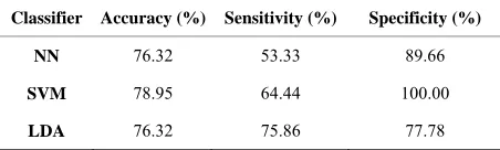
measure the performance of the three classifiers, regard- ing their ability to classify clusters of microcalcifications. Once again, overall accuracy, sensitivity and specificity were measured for each classifier. Table 5 shows the
results of the cross-validation process, in which we can see that the SVM obtained a higher overall accuracy than the other methods and also the highest specificity. On the other hand, the LDA had the best sensitivity while the other two algorithms presented a much lower perform-ance regarding this parameter. In conclusion, the SVM and LDA clearly outperformed the NN in all parameters. However, it should be noted that the sensitivity of the SVM and NN was too low when compared to their other parameters.
6. Results for Masses
The same process performed in the feature selection and classification regarding microcalcification clusters was replicated for the detected masses, considering the afore- mentioned mass-related features and parameters of ex-perimentation.
In Table 6 we provide the results of the feature selec-
[image:7.595.310.536.293.361.2]tion process. It can be observed that the LDA had the highest over-all accuracy but the SVM outperformed all others regarding sensitivity and specificity, having an overall accuracy slightly lower than the LDA. Once again, the NN was outperformed in all three parameters.
Table 7 presents the set of selected mass-related fea-
tures, which represent the best individual found in the GA-based feature selection process, for each of the three classifiers of interest. The NN required 9 features, repre- senting the smallest subset required by the classifiers of interest, while the SVM and LDA used 26 and 20, re- spectively.
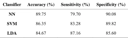
Finally, Table 8 shows the results of the 10-k cross-
validation process. It can be observed that in this case the
Table 5. Cluster-classification performance.
Classifier Accuracy (%) Sensitivity (%) Specificity (%)
NN 76.32 53.33 89.66
SVM 78.95 64.44 100.00
[image:7.595.310.537.392.459.2]LDA 76.32 75.86 77.78
Table 6. Feature selection results for masses.
Classifier Accuracy (%) Sensitivity (%) Specificity (%)
NN 78.05 62.50 88.00
SVM 92.47 92.86 100.00
[image:7.595.310.537.459.738.2]LDA 93.75 83.33 98.73
Table 7. Number of selected mass-features.
Classifier Selected Cluster Features
NN (9 features)
Maximum gray level, minimum gray level, mean gray level, perimeter, strength, shape factor, compactness 2, compactness 3, contour sequence, sequence moment 2.
SVM (26 features)
Minimum gray level, Mean gray level, Standard deviation of the gray level, Kurtosis of gray level, Median gray level, Background Mean gray level, Background Kurtosis of gray level, Relative contrast, Portional contrast, Area, Background area, Filled area, Perimeter, minimum diameter, eccentricity, Roundness, compactness 1, compactness 3, Contour sequence moment 1, contour sequence moment 2, contour sequence moment 3, contour sequence moment 4, Invariant moment 2, invariant moment 4, invariant moment 7.
LDA (20 features)
Table 8. Mass-classification performance.
Classifier Accuracy (%) Sensitivity (%) Specificity (%)
NN 89.75 79.70 90.08
SVM 86.35 83.28 89.82
LDA 84.67 87.16 85.60
NN outperformed the other methods regarding overall accuracy and specificity. On the other hand, LDA pre- sented the highest sensitivity, while the other two algo- rithms presented a much lower performance regarding this parameter. The SVM in this case did not presented the best performance in any of the measured parameters, but still the results obtained with this classification algo- rithm are competitive and provide evidence for the fact that this technique is suitable for our mass-classification stage.
7. Conclusions
In this research effort we developed a CAD model that is able to automatically detect and diagnose clusters of mi- crocalcifications and masses, which are lesions that are evidence of breast cancer.
A large set of features was extracted from ROIs con- taining lesions aimed at describing its visual content. Then, a feature selection process based on a wrapper technique with a GA was performed to find the subsets of features that provide the highest discriminant power for classifying between benign and malignant cases. All three classifiers of interest presented a high performance in this stage.
The final classification stage provides results that show the performance of each method of interest, in which we can observe that they presented a higher per- formance in classifying masses than in the classification of clusters of microcalcifications.
Future work will include research towards the en- hancement of the classification process, by considering different features extracted from ROIs, in order to have a wider experimentation platform to determine which com- bination of features result in a higher performance. Addi- tionally, a training mechanism will be design with the objective of using the database of cases to retrain or modify the internal parameters of the classifiers in an on-line basis.
8. Acknowledgements
This research effort was supported by the Evolutionary Optimization Research Group of Tecnológico de Mon- terrey and the National Council for Science and Tech- nology (CONACyT), under grant 41515.
REFERENCES
[1] C. Tukington and K. Krag, “Encyclopedia of Breast Can-cer,” Facts on File Library of Health and Living, 2005. [2] American Cancer Society, “The Importance of Finding
Breast Cancer Early,” 2012.
http://www.cancer.org/Cancer/BreastCancer/MoreInform ation/BreastCancerEarlyDetection/breast-cancer-early-det ection-importance-of-finding-early
[3] National Cancer Institute. Breast Cancer Screening, 2012. http://www.cancer.gov/cancertopics/pdq/screening/breast/ healthprofessional/page4
[4] S. Ciatto, M. Del Turco, G. Risso, S Catarzi, R. Bonardi, V. Viterbo, P. Gnutti, B. Guglielmoni, L. Ponelli, A. Pan-discia, F. Navarra, A. Lauria, R. Palmiero and P. Indovina, “Comparison of Standard Reading and Computer Aided Detection (cad) on a National Proficiency Test of Scr- eening Mammography,” European Journal of Radiology, Vol. 45, No. 2, 2003, pp. 135-138.
doi:10.1016/S0720-048X(02)00011-6
[5] S. N. Deepa and B. A. Devi, “A Survey on Artificial In-telligence Approaches for Medical Image Classification,” Indian Journal of Science and Technology, Vol. 4, No. 11, 2011, pp. 1583-1595.
[6] M. A. Kumar and H. S. Sheshadri, “On the Classification of Imbalanced Datasets,” International Journal of Com-puter Applications, Vol. 44, No. 8, 2012, pp. 1-7. [7] M. Rizzi, M. D’Aloia and B. Castagnolo, “Health Care
CAD Systems for Breast Microcalcification Cluster De-tection,” Journal of Medical and Biological Engineering, Vol. 32, No. 3, 2012, pp. 147-156.doi:10.5405/jmbe.980 [8] X. S. Zhang, X. B. Gao and Y. Wang, “MCs Detection
with Combined Image Features and Twin Support Vector Machines,” Journal of Computers, Vol. 4, No. 3, 2009, pp. 215-221.doi:10.4304/jcp.4.3.215-221
[9] I. Zyout, I. Abdel-Qader and C. Jacobs, “Embedded Fea-ture Selection Using Pso-Knn: Shape-Based Diagnosis of Microcalcification Clusters in Mammography,” JUSPN, Vol. 3, No. 1, 2011, pp. 7-11.
doi:10.5383/JUSPN.03.01.002
[10] H. D. Cheng, X. J. Shi, R. Min, L. M. Hu, X. P. Cai and H. N. Du, “Approaches for Automated Detection and Classification of Masses in Mammograms,” Pattern Rec- ognition, Vol. 39, No. 4, 2006, pp. 646-668.
doi:10.1016/j.patcog.2005.07.006
[11] A. R. Dominguez and A. F Nandi, “Enhanced Multi- Level Thresholding Segmentation and Rank Based Re- gion Selection for Detection of Masses in Mammo- grams,” IEEE International Conference on Acoustics, Speech and Signal Processing, Vol. 1, 2007, pp. 449-452. [12] S. Singh and K. Bovis, “A Weighted Gaussian Mixture
Model with Markov Random Fields and Adaptive Expert Combination Strategy for Segmenting Masses in Mam-mograms,” Chapter 8, SPIE Press,Bellingham, 2006, pp. 263-289.
82-95.doi:10.1016/j.media.2005.03.007
[14] B. Verma and J. Zakos, “A Computer-Aided Diagnosis System for Digital Mammograms Based on Fuzzy-Neural and Feature Extraction Techniques,” IEEE Transactions on Information Technology in Biomedicine, Vol. 5, No. 1, 2001, pp. 46-54.doi:10.1109/4233.908389
[15] S. E. Conant-Pablos, R. R. Hernández-Cisneros and H. Terashima-Marin, “Feature Selection for the Classifica- tion of Digital Mammograms using Genetic Algorithms, Sequential Search and Class Separability,” In: S. Smith and S. Cagnoni, Eds., Genetic and Evolutionary Compu- tation: Medical Applications, Wiley, New York, 2010. doi:10.1002/9780470973134.ch5
[16] E. Cantú-Paz, “Feature Subset Selections, Class Separa- bility and Genetic Algorithms,” Proceedings of the Ge- netic and Evolutionary Computation Conference, Springer- Verlag, Berlin, 2004, pp. 957-970.
[17] E. Cantú-Paz, S. Newsam and C. Kamath, “Feature Se- lection in Scientific Applications,” Proceedings of the 2004 ACM SIGKDD International Conference on Know- ledge Discovery and Data Mining, ACM, New York, 2004, pp. 788-793.
[18] L. Hadjiiski, B. Sahiner, H. P. Chan, N. Petrick, M. A. Helvie and M. Gurcan, “Analysis of Temporal Changes of Mammographic Features: Computer-Aided Classifica-tion of Malignant and Benign Breast Masses,” Medical Physics, Vol. 28, No. 11, 2001, pp. 2309-2317.
doi:10.1118/1.1412242
[19] R. R. Hernández-Cisneros and H. Terashima-Marín, “Evolutionary Neural Networks Applied to the Classifi-cation of MicrocalcifiClassifi-cation Clusters in Digital Mammo-grams,” Proceedings of the 2006 IEEE Congress on Evo-lutionary Computation, Vancouver, 16-21 July 2006, pp. 2459-2466.
[20] Y. Guo, L. S. Kang, F. J. Liu, H. S. Sun and L. L. Mei, “Evolutionary Neural Networks Applied to Land-Cover Classification in Zhaoyuan, China,” IEEE Symposium on Computational Intelligence and Data Mining, Honolulu, 1-5 April 2007, pp. 499-503.
doi:10.1109/CIDM.2007.368916
[21] T. Deserno, “Biomedical Image Processing,” Springer Verlag, Berlin, 2011.doi:10.1007/978-3-642-15816-2 [22] J. Bozek, M. Mustra, K. Delac and M. Grgic, “A Survey
of Image Processing Algorithms in Digital Mammogra-phy,” Recent Advances in Multimedia Signal Processing and Communications, Vol. 231, Springer, Berlin, 2009. doi:10.1007/978-3-642-02900-4_24
[23] S. Haykin, “Neural Networks: A Comprehensive Founda-tion,” 2nd Edition, Macmillan College Publishing Co., New York, 1999.
[24] V. Vapnik, “Statistical Learning Theory,” John Wiley & Sons, New York, 1998.
[25] T. Hastie, R. Tibshirani and A. Buja, “Flexible Discrimi- nant Analysis by Optimal Scoring,” Journal of the Ameri- can Statistical Association, Vol. 89, No. 428, 1994, pp. 1255-1270.doi:10.1080/01621459.1994.10476866 [26] T. Hastie, R. Tibshirani and J. Friedman, “The Elements
of Statistical Learning. Data Mining, Inference, and Pre- diction,” 2nd Edition, Springer Series in Statistics, Springer, Berlin, 2008.
[27] J. Suckling, J. Parker and D. Dance, “The Mammographic Image Analysis Society Digital Mammogram Database,” Exerpta Medica, International Congress Series 1069, 1994, pp. 375-378.