A b s t r a c t. The aim of this work is to present a fast and cheap method for high-resolution mapping of calcic horizons in vineyards based on geoelectrical proximal sensing. The study area, 45 ha lo-cated in southern Sicily (Italy), was characterized by an old, par-tially dismantled marine terrace and soils with a calcic horizon at different depths. The geoelectrical investigation consisted of a sur-vey of the soil electrical resistivity recorded with the Automatic Resistivity Profiling-03 sensor. The electrical resistivity values at three pseudo-depths, 0-50, 0-100 and 0-170 cm, were spatialized by means of ordinary kriging. A principal component analysis of the three electrical resistivity maps was carried out. During the sur-vey, 18 boreholes, located at different electrical resistivity values, were made for soil description and sampling. The depth to the calcic horizon showed a strong correlation with electrical resisti-vity. The regression model between calcic horizon and the princi-pal component analysis factors with the highest correlation coeffi-cients was selected to spatialise the calcic horizon values. An Normalized Difference Vegetation Index map was used to validate the calcic horizon map in terms of crop response to different soil rooting depths. The strengths of this method are the quick, non-in-vasive kind of survey, the relevance for vine vigour, and the high spatial resolution of the final map.
K e y w o r d s: precision viticulture, soil conservation, irriga-tion, Mediterranean, geophysics
INTRODUCTION
Understanding functional soil features at high spatial resolution is of utmost importance for ‘site-specific’ crop management. In Mediterranean countries, the depth of the upper boundary of the calcic horizon (Dk), described as BCk or Ck, usually corresponds to the soil rooting depth, and thus plays a key role in determining soil fertility and crop water availability. These horizons are usually brought near the surface by erosion processes or incorrect land levelling and
land preparation for the vineyard, which can lead to severe soil degradation (Martínez-Casasnovas and Ramos, 2006) and even desertification (Sánchezet al., 2004).
For this reason, a high-detail map of soils and soil depth is necessary for correct land preparation, vineyard hus-bandry and soil conservation practices within vineyard (Usonet al., 1998). In addition, this kind of investigation is essential for proper and economically sustainable planning of irrigation, tailored to the spatial variability of soil water retention capacity and soil depth.
In particular, it is well known that both the quantity and quality of grapes in the Mediterranean region are signifi-cantly determined by water supply (Costantiniet al., 2006; Deloireet al., 2004). Plant water stress is primarily condi-tioned by rainfall and crop management, but also by rooting depth and soil water retention capacity (Costantiniet al., 2010). Variations in soil properties, often associated with a variation in topography, appear to be a crucial factor in va-riability of vine vigour (Bramley and Lamb, 2003).
Bramley and Lanyon (2002) demonstrated that yield variation in Australian vineyards with a ‘Terra Rossa’ soil (red clayey soil) over limestone was driven by disparity in the water available in the root zone, which in turn was con-trolled by topography variations. Moreover, Bramley and Hamilton (2004) showed that the pattern of the yield varia-tion was closely correlated with soil properties, much more than the influence of seasonal differences.
In the last decade, on-the-go measurement of the spatial variability of the apparent soil electrical conductivity (ECa), or resistivity (ER) has become an invaluable tool to map physical and hydrological parameters of soils. Originally used to investigate soil salinity (Doolittleet al., 2001), this technology has also been used in the last two decades in new investigative fields related to physical and hydrological parameters of soils.
Int. Agrophys., 2013, 27, 313-321 doi: 10.2478/v10247-012-0100-0
Using the ARP-03 for high-resolution mapping of calcic horizons**
S. Priori*, M. Fantappi
è
, S. Magini, and E.A.C. Costantini
CRA-ABP, Italian Agricultural Research Council, Research Center for Agrobiology and Pedology, Piazza M. D’Azeglio 30, 50121, Firenze, Italy
Received October 9, 2012; accepted April 10, 2013
© 2013 Institute of Agrophysics, Polish Academy of Sciences *Corresponding author e-mail: [email protected]
**This work was supported by Sicily region and the Italian Ministry of Agriculture and Forestry with the ‘Valpedo’ 2009-2010 and ‘Issuovino’ (2010-2011) projects.
A A
In recent years, proximal sensing methods have also been used in preliminary studies for precision viticulture. Taylor et al. (2009) used proximal sensing methods and spatial statistics to replace traditional soil maps of vineyards with new high-resolution soil maps. Bourennane et al. (2012) used the principal component analysis (PCA) of electrical resistivity (ER) data to estimate the soil water content in a vineyard.
The aim of the present study was to validate a fast and cheap method for high-resolution soil mapping based on proximal sensing and factorial analysis. The method com-bined the results provided by a geophysical proximal sensor with those from the description of a limited number of bor-ings to obtain a high spatial resolution map of the calcic hori-zon depth in the studied vineyards. The strengths of the method are the quickness and the limited manpower needed to obtain a very high-resolution soil map of the vineyards.
MATERIALS AND METHODS
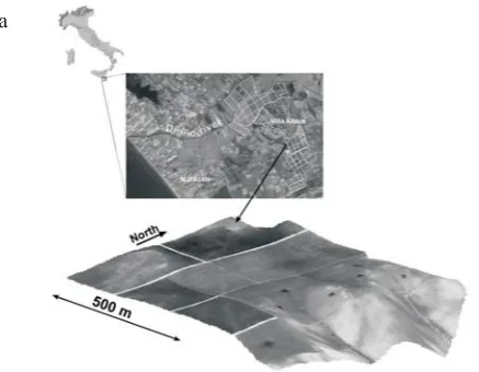
The study area was inside one of Sicily largest wineries, ‘Villa Albius’, situated between Acate and Marina d’Acate (Ragusa) in south-eastern Sicily (Fig. 1). The farm covers about 1 000 hectares, 800 of which are used for irrigated viticulture. It produces indigenous varietals such as Nero d’Avola, Inzolia, Grillo, Frappato, as well as international varietals such as Chardonnay, Syrah and Cabernet Sauvig-non. For this study, ten vineyards (in total 45 ha) were chosen for a detailed proximal sensing survey. The main cultivar in these vineyards was Nero d’Avola, although two small vineyards of Frappato were also present.
Agriculture is the main business in the area and involves frequent soil cultivation to control weeds to prevent water and nutrient competition. The vineyards are located on a broad Plio-Pleistocene marine terrace, a widespread geomorpho-logic unit in this area of Sicily, as in many other Mediterra-nean environments. This terrace is characterized by a first level of calcarenite, a few meters thick and dating to the
Early-Middle Pleistocene, overlying yellow sands partially cemented by calcium carbonate attributed to the Early Pleis-tocene (Grasso, 2000). The terrace is deeply cut by fluvial valleys and strongly eroded, especially along the outer edges.
Some of the vineyards investigated in this study are situated on flat surface of the terrace, characterized by reddish soils developed on the calcarenite. The vineyards situated in the eastern part of the study area, on the slopes of the terrace edge, exhibited either strongly eroded yellowish soils (loose and poorly weathered) developed on the yellow sands, or thin reddish soils developed on the patches of calcarenite residues.
The slopes are very irregular, being cut by small valleys with NW-SE and SE-NW directions, and have different aspects. Moreover, the slopes usually show strong erosion, sometimes in the form of rills and gullies. In contrast, in the vineyards on the terrace, the relatively flat morphology limited soil erosion, with the exception of the small rises, where moderate sheet erosion was active.
The 1:250 000soil map of Sicily (Fantappièet al., 2010) reported the Soil Typologic Units (STUs) of the marine ter-races of the study area: soil region 62.2, described as hills of Sicily on clayey flysch, limestone, sandstone and gypsum, and coastal plains with Mediterranean subtropical climate (Costantiniet al., 2004). In the studied vineyards, the soil map of Sicily reported Endoleptic Calcisols (STU 62.2CLha1) on the slopes of the terrace and Haplic Cambi-sols (STU 62.2CMeu1) on the flat surface of the terrace.
Boundary conditions of the experiment (climate, topo-graphy, vineyard management, rootstock, etc.) could be considered representative of the study area and typical of Mediterranean viticulture on soils formed from homogene-ous bedrock of marine calcarehomogene-ous rocks.
The soil proximal survey of the vineyards was carried out with the ARP-03 (Automatic Resistivity Profiling), a mo-bile soil electrical resistivity mapping system consisting of a multiprobe system of three arrays, provided with a GPS and pulled by an ATV vehicle. The ARP-03, produced since
Fig. 1.Study area – a, extract of the soil map of Sicily – b (1:250 000).
2001, represents the innovation of the MuCEP (Multi Continuous Electrical Profiling) prototype (Panissodet al., 1997; Tabbaghet al., 2000). Both instruments were con-ceived by Geocarta (France), a spin-off society of the CNRS (National Scientific Research Centre, France), for applica-tions in archaeology (Papadopouloset al., 2009) and preci-sion agriculture (Michotet al., 2007).
The ARP-03 device consisted of pairs of toothed metal wheels operating as injection electrodes and three pairs of toothed metal wheels functioning as receivers and measu-ring the difference in electrical potential. The shape of the toothed wheels assured contact between the electrodes and the soil matrix. The distance between each pair of receivers was conceived and calibrated to investigate three soil pseudo-depths, about 0-50 (ER50), 0-100 (ER100) and 0-170 cm (ER170). The measurements of apparent electrical resistivity (ER) in
Wm and the altitude (z) were georeferenced with a GPS and recorded on a field laptop computer.
During the survey, the ARP-03 swaths were spaced about 20 m apart, every 8-9 vine rows, and the total ER data numbered about 4 500 for each pseudo-depthieabout 100 measurments per hectare. This was a good compromise be-tween spatial accuracy and costs, as demonstrated by Andrenelliet al. (2010) and Costantiniet al. (2009). The ra-pidity of the survey was one of the strengths of this method-ology: the proximal survey and the borings for soil des-cription and sampling were conducted by only two people in a single day, 23 March 2010.
The ER data recorded with the ARP-03 were interpo-lated by ordinary kriging with a Gaussian variogram model, using the ArcGIS 9.3 geostatistical analysis (ESRI, Inc., California, USA). The lag distance was 10 m and the maxi-mum range 120 m. In the same way, the altitude data (z), measured by GPS, were used to prepare a detailed 1 x 1 m grid Digital Elevation Model (DEM) of the vineyards.
On the day of the ARP-03 survey, 18 soil borings were carried out with a hand auger up to 1.2 m depth. The location of the borings was chosen on the basis of the ARP-03 results to provide reasonable coverage of the ER values. The soils at the boring sites were described according to NRCS-USDA-NSSC (1998) and 13 of them were sampled for the labora-tory analysis. Particular attention was given to textural chan-ges, pedofeatures (clay coatings, CaCO3nodules and conc-retions), and depth of the horizon boundaries. All soils showed a poorly structured calcic horizon at different depths, described as BCk or Ck. The boundary between the calcic horizon and the overlying Ap, Bw or Bt horizons was always clear. The Dk was very variable. In the shallowest and most eroded soils, a Ck horizon outcropped at the surface.
Laboratory analyses were performed on 10 samples (Ap and subsurface horizons) to characterize the soils according to the official Italian methods (Mi.P.A.F., 2000). Soil texture was determined with a sieve and hydrometer. CaCO3concentration was measured gas-volumetrically by
the addition of HCl in a Dietrich-Frühling calcimeter. EC was measured in 1:2 soil/water solution. Organic carbon was determined by the Walkley-Black procedure. Soil water content (qw) was determined by the thermo-gravimetric method after drying at 105° C for 24 h. The available water capacity (AWC) was estimated with SPAW software (http:// hydrolab.arsusda.gov) which applies the prediction equa-tions of Saxton and Rawls (2006). The laboratory analysis, together with the field descriptions, were used to classify the soil borings according to WRB (IUSS Working Group WRB, 2006) and to group them into Soil Typological Units (STUs).
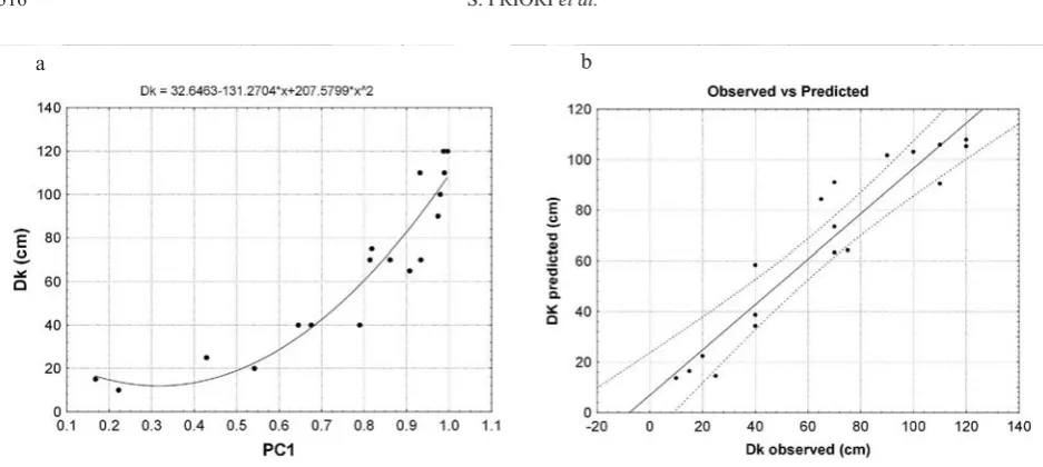
To eliminate multicollinearity of the three ER maps (ER50, ER100and ER170) prior to the regression analysis, a Principal Component Analysis (PCA) was performed by SAGA-Gis, using the variance-covariance matrix. Bouren-nane et al. (2012) used this method in the same way for electrical resistivity data. PCA converts a set of possible correlated variables into a set of uncorrelated values called principal components, namely PCs (Jolliffe, 1986). The PCs are ordered by decreasing explained variance and most of the variance is usually explained by the first few PCs. In our case, we only needed to use the map of PC1, which ex-plained 98.15% of the variance. The map of PC1 was stan-dardized to the range of 0-1 by subtracting the minimum value and dividing by the maximum one in order to avoid negative values. The standardized PC1 values correspond-ing to the borcorrespond-ing locations were extracted to perform the re-gression analysis with the measured Dk values. Linear, power, logarithmic, exponential and polynomial regression models were elaborated to identify the best fitting model to correlate Dk to PC1. A polynomial model was used for the regression analysis (Fig. 2). The regression model was used to interpolate the Dk on the basis of the PC1.
To validate the results of the Dk regression modelling, we used a Normalized Difference Vegetation Index (NDVI) map created with satellite remote sensing as the response va-riable. In fact, it is well known that there is a strong influen-ce of soil depth on plant vigour. An NDVI map is a quick synthetic estimate of spatial variability of the Leaf Area Index (LAI) and thus of crop vigour (Johnsonet al., 2003). A GeoEye-1 multispectral satellite image was acquired to calculate the NDVI map of the vineyards. The image was acquired with the satellite sensor on June 23, 2010, during the veraison period of the grapes. The GeoEye-1 satellite sensor was developed by GeoEye (U.S.) and launched in September 2008. It is capable of acquiring image data at a re-solution of 0.41 m and 1.65 m, respectively, for panchro-matic (B and W) and multispectral images. The Imagine software package (ERDAS Inc., Atlanta, USA) was used for image processing. The NDVI real number outputs (from -1 to +1) were scaled and converted to a byte-binary format 0-255 by the software.
grape-vine phenology. According to Bramley and Lamb (2003), the range time of +/- 2 weeks from veraison is the best predictor of fruit colour and phenolics at vintage. Since the veraison period for the Nero d’Avola cultivar is in the middle or in the second half of July, we acquired a satellite image at the end of June.
After spatialization of the Dk values and validation with the NDVI, a high-detail Soil Typological Units (STUs) map was created, grouping the Dk map into four classes. The Dk limits used for the STUs map were chosen on the basis of the soil typologies identified from the borings.
RESULTS
The ARP-03 provided 4 448 soil electrical resistivity (ER) values for three depths (0-50, 0-100 and 0-170 cm). The interpolated maps of the ER data showed a root mean square error (RMSE) of 25.5, 16.9, 40.5 Wm for ER50, ER100and ER170respectively. The mean values of the ER maps are reported in Table 1. The maps of the data inter-polation are reported in Fig. 3, while the descriptive statistics of the ER data are in Table 1.
The differences in absolute values were clearly visible, especially in the high resistivity areas. ER100 gave the lowest mean value (82.6 Wm) and the lowest standard deviation (93.9Wm). The ER maps showed very similar patterns and were highly correlated among themselves, with R2between 0.916 (ER50with ER100) and 0.935 (ER50with ER170). The PC1 explained 98.15% of the total variance (Table 2). The PC1 map is presented in Fig. 4.
The borehole soil observations revealed a poorly struc-tured, sandy, calcic horizon at variable depths overlying the bedrock, namely the fractured limestone or the partially cemented yellow sands (R or Cr horizon). In some cases, the boreholes were not deep enough to detect the bedrock which was deeper than 1.2 m. In contrast, the calcic horizon (BCk or Ck) was identified in all the soil borings, either over the limestone or on the yellow sands. The BCk or Ck horizon was clearly recognisable from its white-yellowish colour, loose structure and frequent CaCO3nodules and soft concen-trations. The upper boundary of the calcic horizon was always clear and characterized by sudden richness of calca-reous nodules and concretions and by a strong reduction of soil structure. The differentiation between BCk and Ck was
Fig. 2.Polynomial model of: a – Dk spatial regression and b – scatterplot of Dk-observed vs. Dk-predicted with the linear correlation fit and 95% confidence.
b a
Parameter Mean n Min Max 25 Percentile 75 Percentile deviationStandard
h (m) 102.0 4448 86.6 107.7 101.4 103.8 3.3
ER50(Wm) 161.9 4448 18.2 985.1 59.4 209.8 159.3
ER100(Wm) 82.6 4448 4.6 652.1 22.1 106.3 93.9
ER170(Wm) 245.2 4448 15.9 1492.3 72.0 312.3 249.1
based on the soil morphological stage: poor (BCk) or absent (Ck) soil structure and presence/absence of the colour change in the parent material. The BCk horizon often passed to the Ck horizon with a gradual or diffuse boundary.
The Pearson correlation coefficients between the Dk and ER data were very high: 0.87, 0.93 and 0.90 (p<0.01) for ER50, ER100and ER170, respectively. The Pearson coefficient between Dk and PC1 was also very high: 0.92 (p < 0.01).
The best regression model between Dk and PC1 (equa-tion) was the polynomial (Fig. 3) which showed a determi-nation coefficient R2
0.90 (p<0.01):
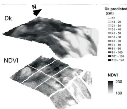
Dk=32.6423-(131.2704 PC1) (207.5799 PC1+ 2) . The root mean square error (RMSE) of the model was 11.5 cm, in relation to a mean Dk value of 75 cm. The model was used to spatialise the Dk values within the studied vine-yards, resulting in the Dk map in Fig. 5.
The cross-correlation between the NDVI and Dk values (Figs 5 and 6) was highly significant (R2= 0.89, p<0.001). The NDVI map showed generally low values in the NE slope, characterized by the most eroded soils, and the highest values in the slight depressions on the flat surface of the terrace where deeper and less eroded soils were more frequent. The comparison between the NDVI and Dk maps allowed us to test the influence of soil depth on vine vigour.
Fig. 3.Interpolated maps of ER50, ER100and ER170.
Parameter PC1 PC2 PC3
ER50 0.506 -0.808 0.301
ER100 0.296 -0.165 -0.941
ER170 0.810 0.565 0.156
Eigenvalue 38634742067 572127498 156528955
% Variance 98.15 1.45 0.4
Cumulative variance
98.15 99.6 100
T a b l e 2.Statistics of the three principal components
Fig. 4.PC1 map. The dots represent the location of borings with the Dk values (cm).
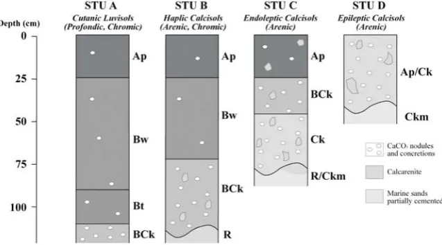
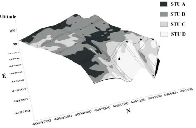
The soil observations made during the survey were grouped into Soil Typological Units (STUs) in order to create a high-detail soil map. On the basis of the field description and laboratory analysis, four STUs (Fig. 7) were identified and classified as follows (IUSS Working Group WRB, 2006): – STU A: Cutanic Luvisol (Profondic, Chromic). This STU
represented the less eroded soils, characterized by a calcic horizon deeper than 100 cm. The soil matrix of the Ap, Bw and Bt horizons was almost completely decarbonated (CaCO3: 0.5%), although some CaCO3hard nodules and some calcarenite fragments were present. The sandy loam texture in the superficial horizons (Ap and Bw) became sandy clay loam in the Bt horizon. The mean AWC was 80 ± 3 mm m-1.
– STU B: Haplic Calcisol (Arenic, Chromic). This STU showed a calcic horizon (BCk) deeper than 75 cm and the bedrock was about 100-120 cm deep. Also in this case the soil matrix of the Ap and Bw horizons was decarbonated (CaCO3: 0.5-1%) with few calcarenite fragments and
CaCO3hard nodules. The texture ranged from loamy sand to sandy loam, and the mean AWC was 57 ± 4 mm m-1. – STU C: Endoleptic Calcisol (Arenic). The upper limit of
the calcic horizon in this STU was shallow (between 25 and 75 cm) and the fractured bedrock was found between 70 and 100 cm. The CaCO3content in the Ap horizon was also high, from 10 to 20%, and CaCO3hard nodules and calcarenite fragments were common. The CaCO3 soft concentrations and nodules became frequent in the BCk horizon, while CaCO3was about 25%. The BCk horizon often changed gradually into the underlying Ck horizon, poorly structured and pale yellowish in colour. The texture was sandy, and the mean AWC was 47± 4 mm m-1. – STU D: Aric Regosol (Calcaric, Arenic). This STU repre-sented the most eroded soils in the vineyards. The calcic horizon was not distinct from the Ap and C horizons be-cause all the horizons had been mixed by deep ploughing. In some cases, a shallow Ap horizon, with poor structure and pale brown in colour, was present, but the Bw soil ho-rizon was absent. The fractured bedrock or the partially cemented unweathered sands were shallower than 50-70 cm. CaCO3concentration of the Ap/Ck horizon was higher than 18% and CaCO3soft concentrations and no-dules were common. The texture was sandy and the mean AWC was 39 ± 4 mm m-1.
The pH (H2O) was sub-alkaline in all soil samples (7.8-8.5) andthe EC varied from about 100 to 188mS cm-1in the superficial horizons (Ap) and from about 30 to 160mS cm-1in the deeper ones (Bw, BCk,etc.). These values in the superficial and deeper horizons excluded the presence of significant soil salinity. The organic carbon was very low in all the soils (< 10 g kg-1). The soil water content (q) was slightly lower than the field capacity for all the samplesand ranged between 1.2 and 11%. As expected, the highest moisture content (8-11%) was always found in the deepest horizons of STUs A and B, while the lower ones were found
Fig. 6.Linear correlation between NDVI and Dk. The error bars show the -90% and +90% quantiles.
in the samples of STU D. The variability of calcic horizon depth, strongly related to soil depth and conservation, was the soil feature that more characterized the STUs variability. The STUs map was developed on the basis of the Dk prediction map (Fig. 8). The Dk limits between STUs was chosen on the basis of the modal value of the calcic horizon depth of each STU, measured during the soil boring de-scriptions. The depth of calcic horizons was below 100 cm for STU A, between 75 and 100 cm for STU B, between 25 and 75 for STU C and shallower than 25 cm for STU D.
DISCUSSION
The ER maps showed very similar patterns, although ER100 had lower mean values and lower standard devia-tions. This was probably due to higher soil water content in the deeper soil horizons, usually located between 30-50 and 90-120 cm. The ER distribution within the study area was characterized by a more resistive area on the slope of the ter-race (North-East of the map) and by less resistive areas on the terraced surface. Although having a similar pattern, the ER170cm map showed higher mean values (243.5Wm) than ER50(160Wm) and ER100(81.7Wm), indicating a high re-sistivity layer in depth. Moreover, the highest ER values were measured on the slopes, where the strongly eroded soils were located. In contrast, the lowest values were typically measured in the flat or slightly concave areas, in the dark red-dish soils that were well-structured and with very scarce gravel.
The PCA confirmed the high correlation and the multicollinearity of the ER values. In fact, PC1 explained 98.15% of the variance, while PC2 and PC3 did not sub-stantially improve the analysis.
The non-linear polynomial regression of Dk with PC1 can be clearly explained by the very strong difference between the electrical resistivity of the upper soil horizons (Ap and Bw) and the bedrock. When the bedrock and the calcic horizon were as shallow as the ARP-03 electrical signal penetration depth, the ER quickly became high. Therefore, a 50 cm deep soil showed an ER value 8-10 times higher than a soil with similar texture but 100 cm deep. This characteristic alone allowed to make a high-resolution spatialization of the Dk within the studied vineyards.
The comparison between the NDVI and Dk maps permitted to test the soil map in terms of the relationship between depth to the calcic horizon and vine vigour. The correlation between the NDVI and Dk values (Figs 5 and 6) was highly significant (R2= 0.89, p < 0.01). Although the NDVI map could not directly validate the Dk predicted map, the strong correlation between these maps supported the accuracy of the spatialization of the Dk values. In fact, the BCk and Ck horizons represented the deepest part of the soil, just overlying the bedrock and with poor structure, low organic matter, low fertility and low water availability. The deeper the calcic horizon, the higher the soil fertility and water retention.
The field description of soil borings and laboratory analysis allowed us to recognise four STUs, distinguished mainly on the basis of the depth to the calcic horizon, strongly related to texture and CaCO3. The results of the other soil analyses, namely pH, EC and OC, were not statistically different between the four STUs. This is due to the great homo-geneity of the area in terms of parent material and land use.
CONCLUSIONS
1. The demonstrated the possibility to use ARP-03 pro-ximal sensors and a few soil boring descriptions for a high-detail map of calcic horizon depth (Dk) in vineyards of SE Sicily (Italy). The Dk prediction map represented the spatial variability of the calcic horizon, closely related to soil depth and conservation.
2. The significant correlation between the Dk and NDVI maps demonstrated a strong relationship between vine vigour and soil depth in the study area.
3. A high-detail Soil Typological Units (STUs) map, derived from the Dk map and a few soil boring descriptions, can be created with a limited amount of fieldwork.
4. The resulting maps of the STUs as discrete variable and Dk as continuous variable can be used to plan a diver-sified field management in terms of fertilization, pruning and irrigation.
REFERENCES
Andrenelli M.C., Costantini E.A.C., Pellegrini S., Perria R. and Vignozzi N., 2010.On-the-go resistivity sensors employ-ment to support soil survey for precision viticulture. Proc. VIII Int. Terroir Congr., June 14-18, Soave, Verona, Italy. Bourennane H., Nicoullaud B., Couturier A., Pasquier C., Mary B., and King D., 2012.Geostatistical filtering for improved soil water content estimation from electrical re-sistivity data. Geoderma, 183-184, 32-40.
Bramley R.G.V. and Hamilton R.P., 2004.Understanding varia-bility in winegrape production systems. 1. Within vineyard variation in yield over several vintages. Australian J. Grape Wine Res., 10, 32-45.
Bramley R.G.V. and Lamb D.W., 2003. Making sense of vineyard variability in Australia. In: Precision Viticulture (Eds R. Ortega A. Esser). Proc. Int. Symp. IX Latin Am. Congr. Viticulture Enology,November 24-28, Santiago, Chile.
Bramley R.G.V. and Lanyon D.M., 2002.Evidence in support of the view that vineyards are leaky. Proc. Workshop Vineyard leakiness, January 24-25, Adelaide, Australia.
Costantini E.A.C., Andrenelli M.C., Bucelli P., Magini S., Natarelli L., Pellegrini S., Perria R., Storchi P., and Vignozzi N., 2009.Strategies of ARP application for viticul-tural precision farming. Proc. E.G.U. Int. Congr., April 19-24, Vienna, Austria.
Costantini E.A.C., Barbetti R., Bucelli P., L’Abate G., Lulli L., Pellegrini S., and Storchi P., 2006.Land peculiarities of the vine cultivation areas in the Province of Siena (Italy), with indications concerning the viticultural and oenological results of Sangiovese vine. Boll. Soc. Geol. It., 6, 147-159. Costantini E.A.C., Pellegrini S., Bucelli P., Barbetti R.,
Campagnolo S., Storchi P., Magini S., and Perria, R., 2010.Mapping suitability for Sangiovese wine by means of d13
C and geophysical sensors in soils with moderate salinity. Eur. J. Agronomy, 33, 208-217.
Costantini E.A.C., Urbano F., and L’Abate, G., 2004. Soil Regions of Italy. http://www.soilmaps.it/download/csi-BrochureSR_a4.pdf.
Deloire A., Carbonneau A., Wang Z., and Ojeda H., 2004.Vine and water: a short review. J. Int. Sci. Vigne Vin, 38, 1-13. Doolittle J.A., Petersen M., and Wheeler T., 2001.Comparison of two electromagnetic induction tools in salinity appraisals. J. Soil Water Conserv., 56, 257-262.
Fantappiè M., Bocci M., Paolanti M., Perciabosco M., Riveccio R., and Costantini E.A.C., 2010.Digital soil mapping of Sicily using G-oriented and CLORPT modelling. Proc. 4th Global Workshop Digital Soil Mapping, May 24-26, Rome, Italy. Grasso M., 2000.Geological context and explanatory notes of the Geological map of the southern-central area of the Iblean plateau.Memorie della Società Geologica Italiana, 55, 45-52.
IUSS Working Group WRB,2006.World Reference Base for soil resource 2006. World Soil Resources Reports No. 103, FAO, Rome, Italy.
Johnson L.F., Roczen D.E., Youkhana S.K., Nemani R.R., and Bosch D.F., 2003. Mapping vineyard leaf area with multispectral satellite imagery. Computers Electronics Agric., 38, 33-44.
Jolliffe I.T., 1986.Principal Component Analysis. Springer, New York, USA.
Lamb D.W., Weedon M.M., and Bramley R.G.V., 2004.Using remote sensing to map grape phenolics and colour in a Caber-net Sauvignon vineyard. The impact of image resolution and vine phenology. Australian J. Grape Wine Res., 10(1), 46-54. Martínez-Casasnovas J.A. and Ramos M.C., 2006.The cost of
soil erosion in vineyard fields in the Penedès-Anoia Region (NE Spain). Catena, 68(2-3), 194-199.
Michot D., King D., Nicoullaud B., Dorigny A., Bourenanne H., Cousin I., Courtemanche P., Couturier A., Pasquier C., Benderitter Y., Dabas M., and Tabbagh A., 2007. Contri-bution of geophysical methods to the knowledge of the spa-tial variability and the hydrological function of the soils (in French). In: Precision Agriculture (Eds M. Guerif, D. King). Quae, Paris, Versailles, France.
Mi.P.A.F,2000.Methods of Soil Chemical Analysis (in Italian). (Ed. F. Angeli), Milan, Italy.
NRCS-USDA-NSSC,1998.Field Book for Describing and Sampl-ing Soils (Eds P.J. Schoeneberger, D.A. Wysocky, E.C. Benham, W.D. Broderson). NRCS-USDA, NSSC, Lincoln, NE, USA.
Panissod C., Dabas M., Jolivet A., and Tabbagh A., 1997.A novel mobile multipole system (MUCEP) for shallow (0-3 m) geoelectrical investigation: the ‘Vol-de-canards’ array. Geophysical Prosp., 45, 983-1002.
Papadopoulos N.G., Tsokas G.N., Dabas M., Yi M.J., Kim J.H., and Tsourlos P., 2009.Three dimensional inversion of Auto-matic Resistivity Profiling data. Archaeological Prosp., 16, 267-278.
region based on soil quality, characteristics and processes. Proc. ISCO 13th Int. Soil Conservation Organisation Conf., July 4-8, Brisbane, Australia.
Saxton K.E. and Rawls W.J., 2006.Soil water characteristic esti-mates by texture and organic matter for hydrologic solu-tions. Soil Sci. Soc. Am. J., 70, 1569-1578.
Tabbagh A., Dabas M., Hesse A., and Panissod C., 2000.Soil resistivity: a non-invasive tool to map soil structure horizo-nation. Geoderma, 97, 393-404.
Taylor J.A., Couluma G., Lagacherie P., and Tisseyre B., 2009. Mapping soil units within a vineyard using statistics asso-ciated with high-resolution apparent soil electrical conduc-tivity data and factorial discriminant analysis. Geoderma, 153, 278-284.