www.geosci-model-dev.net/1/53/2008/
© Author(s) 2008. This work is distributed under the Creative Commons Attribution 3.0 License.
Geoscientific
Model Development
A description of the FAMOUS (version XDBUA) climate model and
control run
R. S. Smith1, J. M. Gregory1,2, and A. Osprey1
1NCAS-Climate, Walker Institute, Reading, UK 2Met Office Hadley Centre, Exeter, UK
Received: 2 July 2008 – Published in Geosci. Model Dev. Discuss.: 28 July 2008
Revised: 2 December 2008 – Accepted: 2 December 2008 – Published: 12 December 2008
Abstract. FAMOUS is an ocean-atmosphere general circu-lation model of low resolution, capable of simulating approx-imately 120 years of model climate per wallclock day using current high performance computing facilities. It uses most of the same code as HadCM3, a widely used climate model of higher resolution and computational cost, and has been tuned to reproduce the same climate reasonably well. FA-MOUS is useful for climate simulations where the compu-tational cost makes the application of HadCM3 unfeasible, either because of the length of simulation or the size of the ensemble desired. We document a number of scientific and technical improvements to the original version of FAMOUS. These improvements include changes to the parameterisa-tions of ozone and sea-ice which alleviate a significant cold bias from high northern latitudes and the upper troposphere, and the elimination of volume-averaged drifts in ocean trac-ers. A simple model of the marine carbon cycle has also been included. A particular goal of FAMOUS is to conduct millennial-scale paleoclimate simulations of Quaternary ice ages; to this end, a number of useful changes to the model infrastructure have been made.
1 Introduction
Computer models are well-established tools for studying the climate system, and the fidelity with which these models can simulate the climate has increased in step with advances in computing power (Randall et al., 2007). However, the large computational cost of high resolution, high complex-ity coupled atmosphere ocean general circulation models
Correspondence to: R. S. Smith ([email protected])
(AOGCM) means that they are usually impractical for studies where millennial timescales are addressed or large ensembles are required. Whilst simplified models which are capable of quickly simulating many thousands of years of climate are available (e.g. Earth System Models of Intermediate Com-plexity (EMIC) Claussen et al., 2002), they often have to omit important processes. To reduce the computational ex-pense of an AOGCM without neglecting any of the processes it describes, one may decrease the spatial resolution and in-crease the timestep of the model. When a computationally cheaper model is closely tied to a more complex AOGCM, the benefits of this approach go beyond simply producing a fast climate model: confidence in the results of the fast model may be gained from the degree to which it agrees with its more sophisticated parent. The fast model can also be used to efficiently explore the parameter space of the parent, and to identify areas where more could be learnt by the applica-tion of the higher resoluapplica-tion version.
A few such low resolution AOGCMs do exist, although they have not yet been very widely used for climate stud-ies. Schurgers et al. (2007) and Vizcaino et al. (2008) have conducted Earth System studies based on a version of the Max Planck Institute ECHAM/LSG model, and Kim et al. (2003) have simulated the Last Glacial Maximum with a ver-sion of the Candian Centre for Climate Modelling and Anal-ysis model. The Community Climate System Model 3 has also been run at a low resolution (Yeager et al., 2006). Also, although not strictly descended from a pre-existing high res-olution coupled model, the FORTE AOGCM has been used for idealised and paleoclimate studies at a low resolution (Smith et al., 2006).
54 R. S. Smith et al.: FAMOUS version XDBUA has been systematically tuned to reproduce both the
equilib-rium climate and climate sensitivity of HadCM3 (Jones et al., 2005). The version of FAMOUS used in Jones et al. (2005) was denoted ADTAN (“adtan” is the UK Met Office Uni-fied Model experiment code for the control run of that model version). Despite the systematic tuning, the climate simu-lated by ADTAN contained a number of biases with respect to HadCM3. Improving the climate of FAMOUS is one of the aims of the UK Quest Earth System Modelling (QUEST-ESM) subproject.
Surface temperatures in ADTAN were too cold north of 50◦N, linked to a persistent overestimate of the amount of sea-ice in this area and too weak northward ocean heat trans-port. Temperatures aloft were also too cold, with an ex-tremely poor representation of the tropopause. ADTAN also did not conserve global ocean salinity, a consequence of the virtual salinity flux boundary condition required by the rigid lid approximation used in the ocean model. Whilst negligi-ble over short timescales, this non-conservation could be a problem during millennial-scale climate simulations.
This paper describes improvements to both the climate and technical infrastructure of FAMOUS contained in the current version, XDBUA. A general overview of FAMOUS is given in Sect. 2, with a more detailed description of the changes since ADTAN in Sect. 3. Section 4 describes the control run of XDBUA. The paper is concluded with a brief discussion and outlook in Sect. 5.
2 Basic FAMOUS
FAMOUS is an AOGCM, based on the widely used HadCM3 (Gordon et al., 2000). FAMOUS uses roughly half the hor-izontal resolution of HadCM3 in both the atmosphere and ocean (along with a longer timestep), so requires only about 10% of the computational resources of HadCM3. Using 8 processors of a linux cluster, FAMOUS can integrate in ex-cess of 100 years per wallclock day, making it suitable for millennial scale climate simulations and ensembles. FA-MOUS has been successfully installed and run on the UK National supercomputing resources HPCx and HECToR, as well as linux-based clusters and desktop machines. ADTAN has been described in Jones (2003) and Jones et al. (2005), but a brief description of the basic components of FAMOUS will be given here for convenience.
The atmosphere component is the Hadley Centre at-mosphere model (HadAM3), a quasi-hydrostatic, primitive equation gridpoint model with a hybrid vertical coordinate (see Pope et al., 2000, for full details). It uses an Eulerian advection scheme, with a gravity-wave drag parameterisation (Gregory et al., 1998). Radiative transfer is modelled us-ing six shortwave bands and eight longwave bands (Edwards and Slingo, 1996; Cusack et al., 1999). Convection fol-lows the mass-flux scheme of Gregory and Rowntree (1990), with parameterisations of convective downdrafts (Gregory
and Allen, 1991) and momentum transport (Gregory et al., 1997). Land processes are modelled via the Met Office Sur-face Exchange Scheme (MOSES1) (Cox et al., 1999) land surface scheme.
In FAMOUS, the horizontal resolution in the atmosphere is 7.5◦longitude×5◦ latitude, with 11 vertical levels. This allows the use of a one hour timestep. The atmosphere and ocean are coupled once every day. Since the resolution of the ocean model is greater than the atmosphere, FAMOUS uses a coastal tiling scheme which combines the properties of land and sea in coastal grid boxes in the atmosphere model. The ocean model can then use the more detailed coastline allowed by its higher resolution grid whilst still conserving coupled quantities. Some of the parameter values in HadAM3 which are poorly constrained by observations have been systemat-ically tuned so that FAMOUS produces a climate more like that of HadCM3 (Jones et al., 2005).
The ocean model is the Hadley Centre ocean model (HadOM3) (see Gordon et al., 2000 for more details), based on the widely used Bryan and Cox code (Bryan, 1969; Cox, 1984). It is a rigid lid model, where surface freshwater fluxes are converted to virtual tracer fluxes via local sur-face tracer values (Pardaens et al., 2003). Temperature and salinity are advected via a simple centred difference method. This has been found to produce better results than more com-plex schemes at climate model resolutions in HadOM3. We use versions of the Gent and McWilliams (1990) and Redi (1982) isopycnal horizontal mixing schemes, with the sur-face mixed layer of Kraus and Turner (1967). Diapycnal mixing below the mixed layer is parameterised using the Richardson-number dependent scheme of Pacanowski and Philander (1981). Convection is modelled via the scheme of Rahmstorf (1993), with Roether et al. (1994) convec-tion being used for addiconvec-tional accuracy in the region of the Greenland-Scotland overflows.
The sea-ice model uses simple, zero-layer thermodynam-ics (Semtner, 1976), with dynamthermodynam-ics based on Bryan (1969). Ice-drifting and leads are parameterised according to Cattle and Crossley (1995). HadOM3 includes the Hadley Centre ocean carbon model (HadOCC), a simple NPZD (Nutrient, Phytoplankton, Zooplankton, Detritus) model of marine bio-geochemistry (Palmer and Totterdell, 2001). HadOCC uses nitrogen as the limiting nutrient, with flows of carbon cal-culated using fixed stoichiometric ratios. There is no trace-element limitation, riverine input or sedimentation, nor are nitrification processes considered. In FAMOUS, HadOCC uses simplified parameterisations of light penetration and self shading (C. Jones, personal communication, 2007), which differ from the original schemes of Palmer and Totterdell (2001). Advection of biogeochemical tracers in XDBUA is done using a flux-limited form of the third-order UTOPIA advection scheme (Leonard et al., 1993), which greatly im-proves the distribution of carbon in the ocean and the resul-tant exchange of carbon dioxide (CO2) with the atmosphere.
FAMOUS has a horizontal resolution of 3.75◦
longitude×2.5◦ latitude in the ocean, with 20 vertical levels. At this resolution, outflow from the Mediterranean is parameterised by simple mixing between an area in the Atlantic and one in the Mediterranean from the surface to a depth of 1300 m. In addition, the low resolution and northern hemisphere cold bias of FAMOUS has led to the removal of Iceland from the model to facilitate ocean heat transport (Jones, 2003). For computational efficiency, the momentum equations are slowed by a factor of 12 (Bryan, 1969), which allows a 12 h timestep to be used. An artificial island is used at the North Pole to avoid the problem of converging meridians, and Fourier filtering is applied at high latitudes to smooth instabilities caused by the long timestep. In HadCM3, a number of the overflows between the North Atlantic and the seas around Greenland, Iceland and Norway were deepened to improve ocean heat transport and deep-water formation; this has not been done in FAMOUS, as it was found to increase the strength of the Atlantic meridional overturning circulation (MOC) too much whilst eliminating the already-weak Antarctic bottom water cell in the Atlantic.
3 Changes
3.1 Orography
The land orography in HadCM3 was derived from the US Navy 10-min resolution dataset, smoothed with a 1-2-1 filter at latitudes poleward of 60◦. The orography used in ADTAN was originally subject to additional smoothing in an attempt to reduce instability in the atmosphere. This instabil-ity was eventually alleviated by extending the filtering of fast atmospheric modes at the poles, so to increase mid-latitude variability in XDBUA the additional orographic smoothing used in ADTAN was removed (Fig. 1). This change in orog-raphy has resulted in a small increase in average eddy kinetic energy in the midlatitude jets (but not instability), and also improves land surface temperatures with respect to HadCM3, as the additional smoothing had lowered the mean topogra-phy in some places. The resultant improvements in surface temperatures can be seen over the Andes, Himalayas and Antarctica, as is discussed in Sect. 4.
3.2 Iceberg calving
The water cycle is not completely represented in FAMOUS: there is a build up of snow on ice-sheets which does not melt, and is not returned to the ocean. In reality this would lead to an increase in the size of the ice-sheet, with the water even-tually being returned to the ocean via iceberg calving, but these processes are not included in FAMOUS. This build-up of snow leads to a slow but steady increase in the salinity of the ocean, which is undesirable in the case of long timescale integrations.
Fig. 1. Land orography used in XDBUA. Above: height above sea-level (metres) for all land points,
includ-ing coastally tiled gridboxes that are considered partially ocean by the atmosphere model; below: difference (metres) from the orography used in ADTAN
23
Fig. 1. Land orography used in XDBUA. Above: height above
sea-level (metres) for all land points, including coastally tiled gridboxes that are considered partially ocean by the atmosphere model; below: difference (metres) from the orography used in ADTAN.
To alleviate this problem, and provide a crude parameter-isation of iceberg calving, an additional surface water flux field has been designed (Fig. 2). The pattern of this field is based on that used in HadCM3 for the same purpose (Gordon et al., 2000). This water flux field has been scaled so that its global integral is such that the global average salinity drift in the modern-day configuration of FAMOUS is cancelled out by its addition. The field is constant, and does not change in response to any changes in ocean salinity drift – it would thus need to be rescaled for use in any model configurations which may have different snow accumulation characteristics, e.g. paleoclimate runs. The volume of snow accumulating on the ice sheets is not changed by the addition of the iceberg field, so the iceberg field represents additional water being introduced to the coupled system. If the accumulated snow were to melt for some reason during a run, a substantial net freshening of the ocean would result.
3.3 Tracer concentration drift
56 R. S. Smith et al.: FAMOUS version XDBUA
Fig. 2. Water flux (kg/m2
/s) applied to the ocean as a simple iceberg calving parameterisation to balance the build up of snow on ice sheets
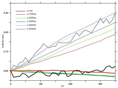
Fig. 3. Global average salinity drifts in FAMOUS. Thin lines are from ADTAN, thick lines are from XDBUA,
with both the freshwater drift adjustment and the iceberg calving fluxes applied. The downward trend in salinity in XDBUA comes from an overestimation of the iceberg flux in this run.
24
Fig. 2. Water flux (kg/m2/s) applied to the ocean as a simple ice-berg calving parameterisation to balance the build up of snow on ice sheets.
to be increased. Using a fixed volume means that freshwa-ter fluxes into the ocean cannot be directly modelled using this approach, so, following common practice, their effect on tracer concentrations are represented by converting the fresh-water flux into a “virtual“ tracer flux. This is usually done one of two ways: either using the local tracer concentration at each gridbox that the flux affects, or by using the same, fixed, reference concentration everywhere. Using local con-centrations gives a more accurate local effect of the fresh-water flux, but it cannot guarantee that the tracer concentra-tion will be conserved globally. This is because the same amount of freshwater will have different effects in different locations: adding an extra Sverdrup of water to an already fresh area will have no effect on the local salinity, but adding it to a very saline area will freshen that gridbox considerably. Calculating the virtual tracer flux instead using a global ref-erence salinity conserves the global tracer concentration - the extra Sverdrup of water will now change the salinity of the fresh and saline gridboxes by the same amount – but at the cost of distorting the local effect of the fluxes, possibly cre-ating negative salinities or inconsistencies in already fresh areas.
It is important to conserve tracers accurately to avoid arti-ficial climate features in long simulations. Whilst HadCM3 conserves global salinity by using a global reference salinity to calculate the surfaces fluxes, ADTAN used local salini-ties, as it was found that the distortion of salinity fluxes that resulted from the use of a global reference value had a signif-icant effect on the strength of the MOC in ADTAN, perhaps because of the lower ocean resolution than HadCM3. Us-ing local salinities to calculate surface tracer fluxes however produced a spurious ocean volume average salinity drift not seen in the surface freshwater budget of ADTAN. As XD-BUA includes biogeochemical tracers, this issue affects more than just the salinity. In XDBUA therefore, a small,
time-Fig. 2. Water flux (kg/m2
/s) applied to the ocean as a simple iceberg calving parameterisation to balance the build up of snow on ice sheets
Fig. 3. Global average salinity drifts in FAMOUS. Thin lines are from ADTAN, thick lines are from XDBUA,
with both the freshwater drift adjustment and the iceberg calving fluxes applied. The downward trend in salinity in XDBUA comes from an overestimation of the iceberg flux in this run.
24
Fig. 3. Global average salinity drifts in FAMOUS. Thin lines are
from ADTAN, thick lines are from XDBUA, with both the fresh-water drift adjustment and the iceberg calving fluxes applied. The downward trend in salinity in XDBUA comes from an overestima-tion of the iceberg flux in this run.
dependent, volume-uniform adjustment is added to each of the tracer fields (salinity, alkalinity and dissolved inorganic carbon) to ensure that the global volume integral concentra-tion of each tracer are conserved.
The adjustment of the tracer fields is calculated as fol-lows. Over the course of a model year, the freshwater fluxes (fwater(x,y,t)) and the virtual tracer fluxes (fvirtual(x,y,t)) at the
surface of the ocean are separately accumulated on every timestep (Fwater=
R
fwaterdt,Fvirtual=
R
fvirtualdt). At the end
of the year, the global drift that should have resulted from the summed freshwater fluxes is calculated for each tracer, using constant global references values (Tref) of 35 psu
for salinity, 2363µmol/l for alkalinity and 2075µmol/l for dissolved inorganic carbon (Dwater=Tref·R Fwaterdxdy).
This is compared with the actual drift in each tracer
(Dvirtual=RFvirtualdxdy), computed from the accumulated
virtual tracer fluxes. A globally constant adjustment is pro-duced for each tracer (A=Dwater−Dvirtual) and the
applica-tion of this adjustment to the tracer field on every timestep of the next year brings the global tracer drift back into line with the surface freshwater forcing. Since the global tracer drift in ADTAN was approximately constant with depth (Fig. 3), to minimise the impact of the adjustment and distortion of spa-tial gradients the drift adjustments A are applied uniformly throughout the depth of the water column.
In the case of a climate with a balanced water cycle, this use of this adjustment will ensure that there is no net ocean tracer drift. Where the climate state has a global net imbal-ance in the freshwater fluxes seen by the ocean – for exam-ple, where there is significant melt of land ice – ocean tracers are allowed to change in line with the global water budget.
HadOCC only considers the impact of freshwater dilution on Alkalinity (Alk) and Dissolved Inorganic Carbon (DIC), not the other tracers (the effect of dilution on concentrations of nutrient, plankton and detritus are considered negligible in the carbon budget). The drift adjustment fluxes in XDBUA are therefore applied only to salinity, Alk and DIC. Changes in global DIC may also result from exchange of CO2
be-tween the atmosphere and ocean, so these are not affected by the adjustment outlined here.
3.4 Sea-ice parameters
ADTAN suffered from a cold bias at high northern latitudes, accompanied by excessive sea-ice (Jones, 2003; Jones et al., 2005). Ice has a positive radiative feedback effect via sur-face albedo, and this obscures the cause of the bias. Analysis showed that ADTAN had a higher surface albedo as a func-tion of sea-ice concentrafunc-tion than HadCM3, suggesting that part of the cold bias may have been caused by unrealistic be-haviour of the sea-ice model at the FAMOUS resolution.
Sea-ice albedo in HadCM3 and FAMOUS is temperature dependent, changing linearly between a low “melting” ice albedo (ALPHAM) and a higher “cold” ice albedo (AL-PHAC) as overlying air temperatures vary between 0 and
−10◦C. This is a crude parameterisation of effects such as the ageing of snow, meltponds, thin ice, and surface contam-ination of old ice which are not modelled explicitly. Sea-ice is also constrained to have a specified depth when new, and to not exceed a maximum concentration (Table 1). Val-ues used for these parameters in ADTAN were determined through earlier tuning experiments in HadCM3.
For XDBUA, these parameters were systematically var-ied in a number of studies aimed at improving the sea-ice distribution and northern hemisphere surface temperature in FAMOUS (the previous tuning efforts by (Jones et al., 2005) only varied parameters in the atmosphere). Following these trials, new values for ALPHAM and the new ice depth have been adopted for XDBUA (Table 1). An albedo of 0.2 is rather low for a large-scale mean, but individual meltponds may have albedoes this low and new, thin ice can be so clear as to effectively have the albedo of the ocean beneath (Al-lison et al., 1992). The new values greatly improve surface temperatures in the northern hemisphere, as is discussed in section 4. In the northern hemisphere, the summer extent of sea ice is much reduced compared to ADTAN, but winter ice extent in the Atlantic is less affected, and ice extent is still generally overestimated in the Pacific (Fig. 4). Sea-ice extent in the Antarctic winter increases slightly, although the sum-mer extent remains unchanged. Surface albedo as a function of sea-ice concentration in XDBUA is generally nearer to that of HadCM3, although the albedo is now too low during northern hemisphere summer.
The climate sensitivity of XDBUA has also changed as a result of these parameter changes. Using the method of Gregory et al. (2004), the climate feedback
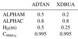
parame-Table 1. Parameter values which have been tuned for the sea-ice
model in XDBUA. ALPHAM and ALPHAC are the albedoes of melting and frozen ice respectively, H0is the thickness of new
sea-ice and CmaxNis the maximum concentration allowed for a northern
hemisphere gridbox.
ADTAN XDBUA ALPHAM 0.5 0.2 ALPHAC 0.8 0.8 H0(m) 0.5 0.25
CmaxN 0.995 0.995
ter, α can be estimated from integrations that have not reached equilibrium by using the balance of fluxes at the top of the atmosphere. Jones et al. (2005) ran integrations with an atmospheric pCO2 of 580 ppmv (twice the
con-trol value) and found α=0.89±0.07 W/m2/K for ADTAN, compared to 1.32±0.08 for HadCM3. An integration of XDBUA using an atmosphericpCO2 of 1160 ppmv found α=1.10±0.09 W/m2/K. Following the usual assumption that
α is largely independent of CO2 forcing, the climate
sen-sitivity of XDBUA has thus been moved closer to that of HadCM3.
3.5 Ozone
Ozone concentrations in HadCM3 are prescribed by a monthly climatology. When interpolated to the lower verti-cal resolution of FAMOUS, this simple scheme meant that a significant rise in the height of the tropopause might result in stratospheric concentrations of ozone being specified in the troposphere, resulting in a water vapour feedback and signif-icant anomalous warming. To avoid this problem, a simple ozone parameterisation was adopted in ADTAN which spec-ified an ozone concentration purely based on whether the gridbox was below, at, or above the diagnosed tropopause (Table 2). This removed the possibility of anomalous tro-pospheric ozone warming, but also underestimated strato-spheric ozone concentrations and warming to the extent that the model often had no tropopause and the stratosphere had a severe cold bias.
High-altitude temperatures have been improved in XD-BUA by the use of a 4-level parameterisation, where, in ad-dition to the 3 categories above, concentrations in the top model level are set to 1.5×10⁻⁶kg/kg, regardless of the
58 R. S. Smith et al.: FAMOUS version XDBUA
XDBUA
HadCM3
XDBUA
HadCM3
DJF
MAM
JJA
SON
1
0.9
0.8
0.7
0.6
0.5
0.4
0.3
0.2
0.1
0
Fig. 4. Seasonal average ice gridbox fractions, XDBUA and HadCM3. Top two rows Northern hemisphere;
bottom two rows Southern Hemisphere.
25
Fig. 4. Seasonal average ice gridbox fractions, XDBUA and HadCM3. Top two rows Northern hemisphere; bottom two rows Southern
Hemisphere.
Table 2. Values for the idealised ozone parameterisations in
AD-TAN and XDBUA. Where the tropopause is found in the top model layer, ADTAN specifies the “At tropopause” value; in XDBUA, the “Top layer” value overrides any other value specified for the top level. The tropopause diagnostic in XDBUA tends to set the tropopause at a lower level, increasing the amount of column ozone.
Level Ozone Conc.(kg/kg) ADTAN XDBUA Top Layer – 1.5×10⁻⁶ Above tropopause 1.5×10⁻⁶ 1.0×10⁻⁶ At tropopause 2.0×10⁻⁷ 2.0×10⁻⁷ Below tropopause 2.0×10⁻⁸ 2.0×10⁻⁸
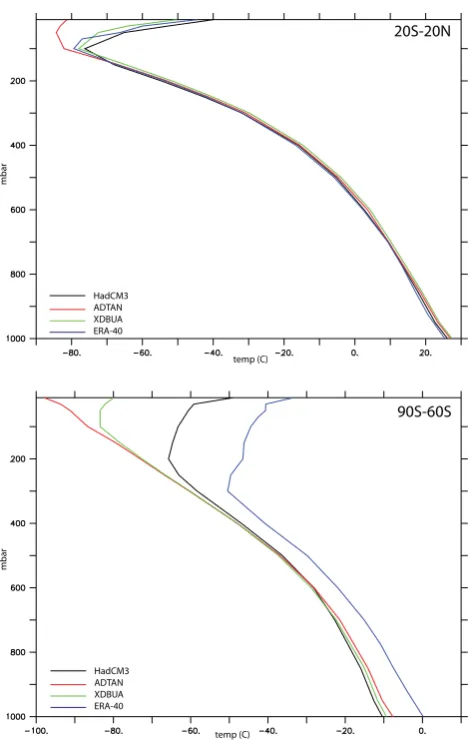
more reliable tropopause in XDBUA, with more realistic ver-tical temperature profiles and improvements in high altitude winds (Fig. 5).
The low vertical resolution at altitude in FAMOUS, which often only has one layer above the tropopause, makes it im-possible to specify realistic ozone concentrations and pro-duce acceptable vertical heating profiles: setting realistic
ozone concentrations at any vertical level in FAMOUS leads to exaggerated longwave absorption and unrealistic heating throughout the air column. Experiments with schemes that shift climatologically-derived ozone concentrations with re-spect to the model tropopause do not show more realistic results than the idealised parameterisation described above, and, at this low resolution, seem less scientifically justifiable. 3.6 Orbital variations
FAMOUS is intended as a platform for long-timescale pa-leoclimate integrations. The UK Met Office Unified Model infrastructure used by FAMOUS was not designed with this sort of experiment in mind, and two new features have been added for use by FAMOUS.
Changes in the strength and seasonality of solar shortwave radiation are important forcings in paleoclimate simulations. FAMOUS now provides a framework for these to be easily specified during an experiment. Both the solar average irra-diance at the top of the atmosphere and the orbital param-eters that control seasonality through eccentricity, obliquity and precession can be changed. Orbitally forced seasonal-ity can either be fixed at a given calendar year, or allowed to
vary with the date through the run. If allowed to vary, the rate at which the orbital parameters change can be artificially accelerated by specifying an acceleration factor greater than 1. For instance, an acceleration factor of 10 would mean that changes in orbital forcing that would normally take 100 years will be applied over 10 model years instead. This accelera-tion has not been used in any results presented here. Users should be aware that acceleration factors should be chosen which are compatible with the timescales of the climate pro-cesses they wish to study. The orbital parameters to be used are calculated via either an online calculation (Berger, 1978) or using published sets of values from extended, offline or-bital calculations. The method implemented for the online calculation is valid for±1 Myr. More recent offline calcula-tions have provided values with some usable accuracy back to 250 Myr B.P. (Laskar et al., 2004).
3.7 Filename format
The standard UM filenaming convention used in ADTAN was designed to provide unique filenames containing date in-formation for runs spanning a few centuries, and were con-strained to be short for compatibility with now-obsolete com-puters. These cryptic names were inconvenient for the long timescales envisaged for FAMOUS, and could be confusing when comparing climate simulations of periods many thou-sands of years apart. A longer, more obvious filenaming con-vention has now been adopted to avoid these problems, that simply places a 9 digit representation of the year in the file-name, with a “−” or “+” suffix to denote whether the year is before or during the Common Era.
4 Control climate
A comprehensive climatology for FAMOUS has not previ-ously been published. We therefore give an overview of some of the climate fields of FAMOUS, compared with both the HadCM3 control run climatology (Gordon et al., 2000) and modern observational data. A control run of XDBUA with a constant atmosphericpCO2of 290 ppmv (representing the
year 1860) has been run for 4000 years. The surface cli-mate is steady, with a trend in global average surface temper-ature of 5.6×10⁻⁴K/yr and a net downward radiative flux at the top of the atmosphere of 0.08 W/m2. These trends are due to the slow adjustment of the deep ocean, and would reduce over a longer spinup run. The climatology of XD-BUA is assessed over 100 years at the end of the control run. A dataset of the climatological surface temperature and precipitation for this period is included as supplementary in-formation to this paper (http://www.geosci-model-dev.net/1/ 53/2008/gmd-1-53-2008-supplement.zip). Where data from ADTAN are used for comparison, they come from a run of FAMOUS conducted by us that has been shown to be statisti-cally identical to Jones et al. (2005)’s original ADTAN state.
mbar
mbar
temp (C)
temp (C) HadCM3
ADTAN XDBUA ERA-40
20S-20N
90S-60S
HadCM3 ADTAN XDBUA ERA-40
Fig. 5. Horizontally averaged vertical temperature profiles (◦C);
above: 20◦S–20◦N; below: 90◦S–60◦S. ERA-40 climatological data comes from Uppala et al. (2005).
Our ADTAN run is, however, only 300 years long and the deep ocean is not as close to equilibrium as in XDBUA.
60 R. S. Smith et al.: FAMOUS version XDBUA
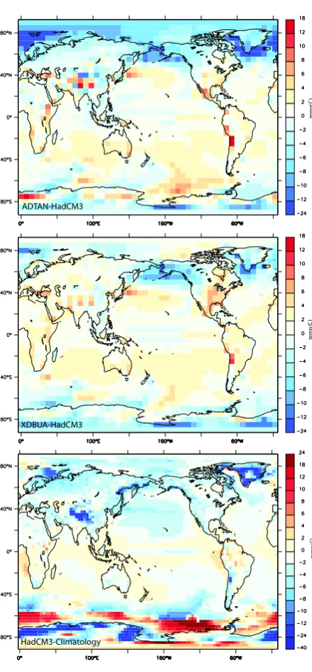
Fig. 6. Annual average surface temperature differences (◦C). Top: ADTAN-HadCM3; middle:
XDBUA-HadCM3; bottom; HadCM3-Legates and Willmott (1990)
27
Fig. 6. Annual average surface temperature differences (◦C). Top: ADTAN-HadCM3; middle: XDBUA-HadCM3; bottom; HadCM3-Legates and Willmott (1990).
of the North American continent in XDBUA, which is due to an intensification of the surface winds bringing warm air north from the Gulf of Mexico. Cold biases remain over the ocean around 60◦N, linked to the persistent overestimate of sea-ice, but the anomalous cooling is not as widespread as it was in ADTAN. In the global average, XDBUA has drifted 0.8◦K further away from HadCM3 than ADTAN, but has replaced ADTAN’s−0.4◦K cold bias with respect to obser-vations with a 0.4◦warm bias.
Table 3. Error in 1.5 m temperature by region. The first line for
each region are differences with respect to HadCM3, the second line are differences with respect to observations (Legates and Will-mott, 1990). The third column shows the change in the size of the absolute error – positive means XDBUA has a larger error than AD-TAN, negative means XDBUA has a smaller error.
ADTAN XDBUA change in absolute error Global 0.53 1.32 +0.80
−0.43 0.36 −0.07
Land Areas
Eurasia 0.11 1.11 +1.00
−3.00 −2.00 −1.00
Africa 1.55 2.00 +0.46 0.98 1.44 +0.46 N. America −1.31 0.19 −1.11
−4.41 −2.91 −1.50
S. America 2.58 2.54 −0.03 1.88 1.84 −0.03 Australia 1.79 2.05 +0.26 1.21 1.47 +0.26 Antarctica −0.03 −0.61 +0.58
−5.84 −6.42 +0.58 Sea Areas
Atlantic 0.12 1.16 +1.04
−0.11 0.93 +0.81 Pacific 0.84 1.41 +0.58 0.00 0.58 +0.58 Indian 1.24 1.93 +0.69 1.49 2.18 +0.69 Arctic −6.49 −1.25 −5.24
−9.26 −4.02 −5.24
Southern 0.97 1.53 +0.56
Ocean 1.31 1.87 +0.56
Precipitation patterns in XDBUA are little changed from ADTAN. The distribution of errors with respect to data (Xie and Arkin, 1997) are similar to those in HadCM3, but are accentuated in FAMOUS. The largest differences are over the tropical oceans, where differences are linked to convec-tion and the Hadley circulaconvec-tion. The Hadley circulaconvec-tion in FAMOUS is too weak and extends too far poleward into the summer hemisphere, leading to a lack of convective rainfall in the tropics and too much in the sub-tropics.
Synoptic variability is generally too weak in AOGCMs (e.g. Osborn et al., 1999), and the low resolution of FA-MOUS results in an underestimate of variability on seasonal to interannual timescales. Storm-tracks are too weak in FA-MOUS (Fig. 8), providing drizzle over the north Atlantic and Europe, rather than storms. This was also the case in AD-TAN, and neither the warmer northern Atlantic climate nor the less smoothed topography of XDBUA has improved the representation of stormtracks in FAMOUS. Transient eddy
Fig. 7. Annual average precipitation (mm/day). Top: XDBUA; middle: XDBUA-HadCM3; bottom:
HadCM3-CMAP (Xie and Arkin, 1997)
28
Fig. 7. Annual average precipitation (mm/day). Top: XDBUA;
middle: XDBUA-HadCM3; bottom: HadCM3-CMAP (Xie and Arkin, 1997).
kinetic energy at the top of the troposphere in the midlat-itudes is still significantly underestimated in XDBUA, but there is a small improvement over ADTAN due to the use of a less smoothed orography.
On interannual scales, the leading empirical orthogonal function (EOF) of northern hemisphere mean sea level pres-sure (MSLP) can be used to characterise the North Atlantic
Fig. 8. 500mbargeopotential height anomalies, 2-6 day bandpass filtered (metres). Top: XDBUA; bottom; ERA-40 (Uppala et al., 2005)
Fig. 9. The leading EOF of annual mean sea level pressure in (left) XDBUA and (right) HadCM3. They explain
21% and 25% respectively of the total variability in each model.
29
Fig. 8. 500 mbar geopotential height anomalies, 2–6 day bandpass
filtered (metres). Top: XDBUA; bottom; ERA-40 (Uppala et al., 2005).
Oscillation or the Arctic Oscillation. XDBUA reproduces the basic features of the tripole of Pacific, Arctic and North At-lantic pressure variations seen in observations and HadCM3 (Fig. 9), with the leading EOF explaining 21% of the to-tal MSLP variability in XDBUA. In XDBUA, the pattern is dominated by Pacific variability, a result of the anomalous winter sea-ice there and the too-weak variability over the North Atlantic already seen. Tropical variability is also much higher in FAMOUS. The leading EOF of MSLP in XDBUA shows some improvement over ADTAN, where Pacific vari-ability totally dominated the EOF and the tripole structure was less evident.
62 R. S. Smith et al.: FAMOUS version XDBUA Fig. 8. 500mbargeopotential height anomalies, 2-6 day bandpass filtered (metres). Top: XDBUA; bottom;
ERA-40 (Uppala et al., 2005)
Fig. 9. The leading EOF of annual mean sea level pressure in (left) XDBUA and (right) HadCM3. They explain
21% and 25% respectively of the total variability in each model.
29
Fig. 9. The leading EOF of annual mean sea level pressure in (left)
XDBUA and (right) HadCM3. They explain 21% and 25% respec-tively of the total variability in each model.
period (yrs)
po
w
e
r
135E 180 135W 90W
10N
0
10S
Fig. 10. Above: Power spectrum of 150 years of a Nino3 index
from XDBUA (black). Red lines show 95% confidence intervals for an AR(1) process fitted to the timeseries. Below: Composite of SST anomaly events (◦C) identified from the 3–5 year bandpass filtered Nino3 index.
timeseries from the Nino3 region (150◦W to 90◦W, 5◦S to 5◦N) in XDBUA suggests that some interannual variability does exist in the Pacific in FAMOUS (Fig. 10). Although the Nino3 index in XDBUA has significant power in the 3–5 year period band, the strong peak at 10 years and the pat-tern of the related composite SST anomaly suggest that the
90S 45S 0 45N 90N
PW 0 2 4
-2
-4
Atmosphere
XDBUA HadCM3 ADTAN
Ocean
Atlantic Global
XDBUA HadCM3 ADTAN
PW
90S 45S 0 45N 90N
0 1
-1
Fig. 11. Above: Atmospheric energy transport (
PW
). Black: HadCM3; Red: ADTAN; green: XDBUA.
Below: Ocean heat transports (
PW
). thin line: Atlantic; thick line: Global. Colours as above.
31
Fig. 11. Above: Atmospheric energy transport (PW). Black: HadCM3; Red: ADTAN; green: XDBUA. Below: Ocean heat transports (PW). thin line: Atlantic; thick line: Global. Colours as above.
oscillation may not primarily be a coupled dynamic feature as in reality, but have significant input from a purely ther-modynamic artificial model mode similar to one detected in HadCM3 (Toniazzo, 2008). Low resolution models often have insufficient vertical resolution in the thermocline to al-low small surface heat anomalies to couple effectively with the atmosphere, and can upwell too much cold water along the equator, which reduces the potential for warm anomalies to survive. The presence of an oscillation on these timescales in the tropical Pacific, whatever its mechanism, is, neverthe-less, a positive sign.
FAMOUS reproduces the meridional energy transports of HadCM3 relatively well (Fig. 11). Atmospheric energy transports are underestimated by around 0.5 PW at their peak in the midlatitudes, most likely due to the lack of midlat-itude variability in FAMOUS. Peak meridional ocean heat transport in the ocean in FAMOUS is about 0.3 PW less than that in HadCM3, with most of this underestimate being found in the Atlantic MOC. This weak ocean heat transport is re-sponsible for some of the persistent cold bias found at high northern latitudes in FAMOUS. Some of the differences in
the MOC between XDBUA and HadCM3 are likely to be due to their different representations of the sill depths be-tween the Greenland-Iceland-Norwegian seas and the North Atlantic.
A useful estimate of the overall climate provided by a model can be gained by looking at what sort of vegetation would be favoured by the climate in different regions of the world. The K¨oppen-Geiger climate zones are defined for this purpose based on the means, ranges and seasonality of temperature and precipitation. They have been evaluated in XDBUA following the criteria set out in Gnanadesikan and Stouffer (2006) (Fig. 12). FAMOUS reproduces the over-all distribution of climate zones found in HadCM3 and the real world well, despite its low resolution. The majority of regions have the correct “main” climate, are about the right size, and in the correct locations. There a few discrepan-cies: in common with HadCM3, the Amazon region is not wet enough for a fully humid region to exist, whilst South Africa and central Australia are too wet for the desert-like conditions they ought to have. In FAMOUS, India is too hot and dry, features that are likely linked to a poor representa-tion of monsoon rainfall that would both wet and cool the surface. North America is represented as a little too warm for the climate zones it should have.
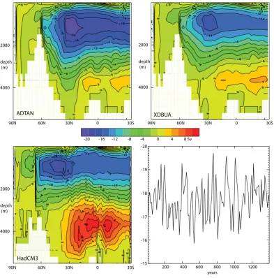
The Atlantic MOC has a mean of 17 Sv and a decadal standard deviation of 0.83 Sv. It is similar to the MOC in HadCM3, but is a little weaker, and does not penetrate as far north (Fig. 13). The difference in the northward extent of the circulations is due to the differences in bottom topog-raphy, which is much shallower in FAMOUS. Compared to HadCM3, FAMOUS also underestimates Antarctic bottom water production and penetration into the North Atlantic, but XDBUA has slightly more Antarctic bottom water than AD-TAN did. This may be linked to a small increase in season-ality around Antarctica resulting from the increase in winter sea-ice extent in XDBUA.
The surface temperature and precipitation fields seen for the atmosphere (Figs. 6 and 7) are reflected in the sea surface temperature (SST) and salinity (SSS) deviations from obser-vations (Fig. 14). The remaining cold bias in surface tem-peratures in XDBUA can be seen in the north Atlantic and Pacific, whilst the small southern hemisphere warm bias in surface air temperature shows up clearly in the SST. Errors in SSS are mostly found round the coasts or under sea-ice where they reflect inaccuracies in runoff or ice formation, al-though the anomalous pattern in the Pacific is closely linked to that of the precipitation in the region, reflecting errors in the model’s Hadley circulation. The pattern of errors in the SSS field can also be seen in both DIC and Alk, reinforc-ing the importance of correctly representreinforc-ing freshwater ex-changes in an Earth System Model. Both the pattern and magnitude of the ocean surfacepCO2 and CO2 exchange
with the atmosphere in this run with fixed 290 ppmv atmo-spheric CO2 are plausible, although no direct observations
of these fields exist for comparison.
Fig. 12. K¨oppen-Geiger climate zones, following Gnanadesikan and Stouffer (2006). Note that boxes are
coloured if there is any land present; coastal boxes have fractional land coverage. Zones are coded using combinations of letters to indicate climatic characteristics: Main climate - A: equatorial; B: arid; C: warm temperate; D: snow; E: polar. Precipitation - W: desert; S: Steppe; f: fully humid; s: summer dry; w: winter dry; m: monsoonal. Temperature - h: hot arid; k: cold arid; a: hot summer; b: warm summer; c: cool summer;
d: extremely continental; F: polar frost; T: polar tundra. Top: XDBUA; middle: HadCM3; bottom; using data
from ERA-40 (Uppala et al., 2005)
32
64 R. S. Smith et al.: FAMOUS version XDBUA
ADTAN
2000
depth (m)
4000
90N 60N 30N 0 30S
XDBUA
90N 60N 30N 0 30S 2000
depth (m)
4000
200 400 600 800 1000 1200 years
-20
-19
-18
-17
-16
-15
HadCM3
2000
depth (m)
4000
90N 60N 30N 0 30S
-20 -16 -12 -8 -4 0 4 8 Sv
Fig. 13. Atlantic MOC (Sv, clockwise rotation is positive). Top left: average of 100 years from ADTAN; top right: Average of 1400 years
from XDBUA; bottom left: climatological average from HadCM3; bottom right: Timeseries of decadal means in XDBUA.
Below the surface, the vertical profiles of ocean tracers in XDBUA (Fig. 14) compare well with observations, in the context of results from HadCM3 and HadCM3LC (Cox et al., 2000) (a version of HadCM3 with a lower ocean resolution, which also uses HadOCC to model the marine carbon cycle). The cold bias found in HadCM3LC is improved, with XD-BUA having a small warm bias at depth. The near-surface fresh bias seen in HadCM3 is improved in XDBUA. The vertical profile of DIC in XDBUA is much better than that simulated by HadCM3LC, where overly cold temperatures allowed too much carbon to be stored at depth. Alk is gen-erally overestimated in both HadCM3LC and XDBUA, al-though the ratios of DIC to Alk are better in XDBUA.
5 Discussion
FAMOUS is a lower resolution version of the HadCM3 cou-pled AOGCM, capable of simulating around 100 years of cli-mate per wallclock day on 8 processors of a linux cluster. This makes it a useful tool which can apply the many pro-cesses and complex feedbacks that an AOGCM is capable of representing to climate simulations that would otherwise be too computationally expensive for other GCMs. The version of FAMOUS described in this paper, XDBUA, has had seri-ous cold biases alleviated at the surface and at the tropopause, and has schemes for cancelling drift in the concentrations of ocean tracers. Its climate sensitivity has also been moved closer to that of HadCM3.
Like any model, FAMOUS still contains errors in its simu-lation of climatic states and changes. For example, although
SST
XDBUA-Climatology
SSS
XDBUA-Climatology
Temperature errors Salinity Errors
DIC Alk
depth (m) depth (m)
depth (m) depth (m)
µmol/l µmol/l
oC
oC
psu
psu
GLODAP HadCM3LC XDBUA
GLODAP HadCM3LC XDBUA
HadCM3 HadCM3LC XDBUA ADTAN HadCM3
HadCM3LC XDBUA ADTAN
Fig. 14. Tracer concentrations in the ocean. Top left: SST errors relative to Levitus et al. (1998); top right: SSS errors relative to Levitus
et al. (1998). Middle left: Horizontally averaged potential temperature errors relative to (Levitus et al., 1998) (black: HadCM3; blue: HadCM3LC; green: XDBUA); red: ADTAN; Middle right: Horizontally averaged salinity errors relative to Levitus et al. (1998) (colours as before). Bottom left: Horizontally averaged DIC (purple: Key et al. (2004); blue: HadCM3LC; green: XDBUA); Bottom right: Horizontally average Alk (colours as before).
zonal mean temperatures match observations and HadCM3 reasonably well, significant errors in surface temperature still exist on the scale of individual gridboxes. However, the im-portance of errors in climate simulation depends on the scien-tific question that you wish to apply the model to; FAMOUS may not be an appropriate tool for simulating regional cli-mate but is well suited to questions involving larger spatial scales. We chose to concentrate on the cold bias and tracer drift in the FAMOUS climate because they represent the most serious obstacles to simulating long term, large scale changes in global climate. For these changes, ice provides a very important positive feedback mechanism. The significant
cold bias in equilibrium climate at high northern latitudes in ADTAN did not provide a realistic base state for simulating changes in ice, so removing that cold bias is important. Over long timescales, small drifts in ocean tracers such as salinity and DIC can have significant effects on the ocean circulation or biogeochemistry as they accumulate over the course of a run, so finding acceptable ways of cancelling this drift was also necessary.
66 R. S. Smith et al.: FAMOUS version XDBUA in CO2is similar to that of HadCM3, this cold bias, and the
over-estimate of sea-ice extent, might distort the model sim-ulation of cold climates, or features such as Heinrich events that involve (possibly abrupt) North Atlantic cooling. Al-though we have not yet simulated such states directly, we have conducted an ensemble of simulations where freshwa-ter is artificially added to the North Atlantic to reduce the strength of the MOC. This ensemble produces a range of MOC responses in line with that found by Stouffer et al. (2006) when they compared similar experiments in a range of coupled AOGCMs, including HadCM3. Our FAMOUS ensemble also produces the same range of surface tempera-ture changes in the North Atlantic region as Stouffer et al. (2006). This suggests that FAMOUS’s ability to simulate rapid cooling events associated with changes in ocean circu-lation is not seriously affected by the remaining cold bias in XDBUA.
With a model such as FAMOUS that is derived from a higher resolution parent, the question arises as to what to use as a reference to judge the model climate. Although real-ity is the ideal benchmark, suitable observations may not ac-tually exist, especially for historical periods. An argument can be made for using the higher resolution model as the reference, as is done in many cases here (and implicitly in Jones et al. (2005)’s tuning); it is, after all, unlikely that the lower resolution model will perform more realistically than the higher resolution one, and the comparison is certainly much easier than using observational data. This approach, however, runs the risk of ignoring biases in the simulation of the parent model. In our case, where possible we have tried to compare FAMOUS to both HadCM3 and observations, al-though for certain variables comprehensive observations do not exist (e.g. the Atlantic MOC). As FAMOUS is expanded into a more complete Earth System model and incorporates processes which HadCM3 did not simulate, the references used for comparison will inevitably have to move away from HadCM3 and be more directly derived from observations.
Variations in atmospheric carbon dioxide and ice sheets are important factors in determining the climate of the Earth, and both participate in a range of feedback with the rest of the climate system. At the moment these features must be prescribed within FAMOUS, and feedbacks with them are not represented. Future work with FAMOUS will focus on modelling ice and carbon dioxide as interactive elements of the climate simulation. The Glimmer (http://glimmer.forge. nesc.ac.uk) model will provide icesheets, whilst the carbon cycle will be closed by the inclusion of the MOSES2.2 land scheme (Essery et al., 2003), which will allow atmospheric
pCO2to vary according to exchange with soils and
vegeta-tion. The TRIFFID dynamic vegetation model (Cox, 2001) will also be included, allowing plant populations to respond to the local climate. More information about FAMOUS and ongoing development work can be found on the website at http://www.famous.ac.uk.
Acknowledgements. We would like to thank the Met. Office
for use of the original FAMOUS code, and Chris Jones, Dave Storkey and Ian Totterdell for advice and extra code. We would also like to acknowledge the support of Simon Wilson and other members of the NCAS Computer Modelling Support Team in this work. The work was supported by grants from the U.K. RAPID (NER/T/S/2002/00462), Quaternary QUEST (NE/D00182X/1) and QUEST-ESM projects. Jonathan Gregory was partly supported by the Integrated Climate Programme, GA01101 (Defra) and CBC/2B/0417 Annex C5 (MoD).
Edited by: D. Lunt
References
Allison, I., Brandt, R., and Warren, S.: East Antarctic Sea-Ice: Albedo, Thickness Distribution, and Snow Cover, J. Geophys. Res, 98, 12 417–12 429, 1992.
Berger, A. L.: Long-term variations of daily insolation and quater-nary climatic, J. Atmos. Sci., 35, 2362–2367, 1978.
Bryan, K.: A numerical method for the study of the circulation of the World Ocean, J. Comput. Phys., 4, 347–376, 1969.
Cattle, H. and Crossley, J.: Modeling Arctic climate-change, Philos. Trans. R. Soc. London, 352, 201–213, 1995.
Claussen, M., Mysak, L., Weaver, A., Crucifix, M., Fichefet, T., Loutre, M.-F., Weber, S., Alcamo, J., Alexeev, V., Berger, A., Calov, R., Ganapolski, A., Goosse, H., Lohmann, G., Lunkeit, F., Mokhov, I., Petoukhov, V., Stone, P., and Wang, Z.: Earth system models of intermediate complexity: closing the gap in the spectrum of climate system models, Clim. Dynam., 18, 579– 586, 2002.
Collins, W. D.: Effects of enhanced shortwave absorption on cou-pled simulations of the tropical climate system, J. Climate, 14, 1147–1165, 2001.
Cox, M. D.: A primitive equation, 3-dimensional model of the ocean, Tech. Rep. 1, Geophysical Fluid Dynamics Labora-tory/NOAA, Princeton University, 1984.
Cox, P., Betts, R., Jones, C., Spall, S., and Totterdell, I.: Accel-eration of global warming due to carbon-cycle feedbacks in a coupled climate model, Nature, 408, 184–197, 2000.
Cox, P. M.: Description of the TRIFFID Dynamic Global Vegeta-tion Model, Technical Note 24, Hadley Centre, Met Office, 2001. Cox, P. M., Betts, R. A., Bunton, C. B., Essery, R. L. H., Rowntree, P. R., and Smith, J.: The impact of new land surface physics on the GCM simulation of climate and climate sensitivity, Clim. Dynam., 15, 183–203, 1999.
Cusack, S., Edwards, J. M., and Kershaw, R.: Estimating the sub-grid variance of saturation, and its parametrization for use in a GCM cloud scheme., Q. J. R. Meteorol. Soc., 125, 3057–3076, 1999.
Edwards, J. M. and Slingo, A.: Studies with a flexible new radiation code. I: Choosing a configuration for a large-scale model., Q. J. R. Meteorol. Soc., 122, 689–720, 1996.
Essery, R. L. H., Best, M. J., Betts, R. A., Cox, P. M., and Taylor, C. M.: Explicit representation of subgrid heterogeneity in a GCM land-surface scheme, J. Hydrometeorol., 4, 530–543, 2003. Gent, P. and McWilliams, J.: Isopycnal Mixing in ocean circulation
models, J. Phys. Oceanogr., 20, 150–155, 1990.
Gnanadesikan, A. and Stouffer, R. J.: Diagnosing atmosphere-ocean general circulation model errors relevant to the terrestrial biosphere using the Koeppen climate classification, Geophys. Res. Lett., 33, L22701, doi:10.1029/2006GL028098, 2006. Gordon, C., Cooper, C., Senior, C., Banks, H., Gregory, J., Johns,
T., Mitchell, J., and Wood, R.: The simulation of SST, sea ice ex-tents and ocean heat transports in a version of the Hadley Centre coupled model without flux adjustments, Climate Dynam., 16, 147–168, 2000.
Gregory, D. and Allen, S.: The effect of convective downdraughts upon NWP and climate simulations, in: Ninth conference on nu-merical weather prediction, Denver, Colorado, 122–123, 1991. Gregory, D. and Rowntree, P. R.: A mass-flux convection scheme
with representation of cloud ensemble characteristics and sta-bility dependent closure, Mon. Weather Rev., 118, 1483–1506, 1990.
Gregory, D., Kershaw, R., and Inness, P. M.: Parametrization of momentum transport by convection II: Tests in single column and general circulation models, Q. J. R. Meteorol. Soc., 123, 1153– 1183, 1997.
Gregory, D., Shutts, G. J., and Mitchell, J. R.: A new gravity wave drag scheme incorporating anisotropic orography and low level wave breaking; Impact upon the climate of the UK Meteorologi-cal Office Unified Model, Q. J. R. Meteorol. Soc., 124, 463–493, 1998.
Gregory, J. M., Ingram, W. J., Palmer, M. A., Jones, G. S., Stott, P. A., Thorpe, R. B., Lowe, J. A., Johns, T. C., and Williams, K. D.: A new method for diagnosing radiative forcing and cli-mate sensitivity, Geophys. Res. Lett., 31, L03205, doi:10.1029/ 2003gl018747, 2004.
Guilyardi, E., Gualdi, S., Slingo, J., Navarra, A., Delecluse, P., Cole, J., Madec, G., Roberts, M., Latif, M., and Terray, L.: Representing El Nino in coupled ocean-atmosphere GCMs: The dominant role of the atmospheric component, J. Climate, 17, 4623–4629, 2004.
Jones, C.: A fast ocean GCM without flux adjustments, J. Atmos. Ocean. Tech., 20, 1857–1868, 2003.
Jones, C., Gregory, J., Thorpe, R., Cox, P., Murphy, J., Sexton, D., and Valdes, P.: Systematic Optimisation and climate simulations of FAMOUS, a fast version of HadCM3, Clim. Dynam., 25, 189– 204, 2005.
Key, R., Kozyr, A., Sabine, C., Lee, K., Wanninkhof, R., Bullister, J., Feely, R., Millero, F., Mordy, C., and Peng, T.-H.: A global ocean carbon climatology: results from the Global Data Analysis Project (GLODAP), Glob. Biogeochem. Cy., 18, GB4031, doi: 10.1029/2004GB002247, 2004.
Kim, S., Flato, G., and Boerm, G.: A coupled climate model simu-lation of the Last Glacial Maximum, Part 2: approach to equilib-rium, Clim. Dynam., 20, 635–661, 2003.
Kraus, E. B. and Turner, J. S.: A one dimensional model of the seasonal thermocline. Part II, Tellus, 19, 98–105, 1967. Laskar, J., Robutel, P., Joutel, F., Gastineau, M., Correia, A. C. M.,
and Levrard, B.: A long-term numerical solution for the insola-tion quantities of the Earth, Astron. Astrophys., 428, 261–285, 2004.
Legates, D. R. and Willmott, C. J.: Mean Seasonal and Spatial Vari-ability in Global Surface Air Temperature., Theor. Appl. Clima-tol., 41, 11–21, 1990.
Leonard, B. P., MacVean, M. K., and Lock, A. P.:
Positivity-preserving numerical schemes for multidimensional advection, Nasa Tech. Memo. 106055, ICOMP-93-05, NASA, Washington, DC, 20546-0001, 1993.
Levitus, S., Boyer, T., Conkright, M., Brien, T. O., Antonov, J., Stephens, C., Stathoplos, L., Johnson, D., and Gelfeld, R., eds.: NOAA Atlas NESDIS 18, World Ocean Database 1998 Volume 1, National Oceanographic Data Center, 1998.
Osborn, T. J., Conway, D., Hulme, M., Gregory, J. M., and Jones, P. D.: Air flow influences on local climate: observed and simu-lated mean relationships for the United Kingdom, Climate Res., 13, 173–191, 1999.
Pacanowski, R. and Philander, S.: Parameterization of vertical mix-ing in numerical models of tropical oceans, J. Phys. Oceanogr., 11, 1443–1451, 1981.
Palmer, J. R. and Totterdell, I. J.: Production and export in a global ocean ecosystem model, Deep-Sea Res., 48, 1169–1198, 2001. Pardaens, A. K., Banks, H. T., Gregory, J. M., and Rowntree, P. R.:
Freshwater transports in HadCM3, Clim. Dynam., 21, 177–195, 2003.
Pope, V. D., Gallani, M. L., Rowntree, P. R., and Stratton, R. A.: The impact of new physical parametrizations in the Hadley Cen-tre climate model – HadAM3, Clim. Dynam., 16, 123–146, 2000. Rahmstorf, S.: A fast and complete convection scheme for ocean
models, Ocean Model., 101, 9–11, 1993.
Randall, D. A., Wood, R. A., Bony, S., Colman, R., Fichefet, T., Fyfe, J., Kattsov, V., Pitman, A., Shukla, J., Srinivasan, J., Stouf-fer, R. J., Sumi, A., and Taylor, K. E.: Climate models and their evaluation, in: Climate Change 2007: The Physical Science Basis. Contribution of Working Group I to the Fourth Assess-ment Report of the IntergovernAssess-mental Panel on Climate Change, chap. 8, 589–662, Cambridge University Press, 2007.
Redi, M. H.: Oceanic isopycnal mixing by coordinate rotation, J. Phys. Oceanogr., 12, 1154–1158, 1982.
Roether, W., Roussenov, V. M., and Well, R.: A tracer study of the thermohaline circulation of the Eastern Mediteranean., in: Ocean Processes in Climate Dynamics: Global and Mediterranean Ex-amples., 371–394, Kluwer Acad. Pub., 1994.
Schurgers, G. ., Mikolajewicz, U., Gro¨ger, M., Maier-Reimer, E., Vizcaino, M., and Winguth, A.: The effect of land surface change on Eemian climate, Clim. Dynam., 29, 357–373, 2007.
Semtner, A. J.: A model for the thermodynamic growth of sea ice in numerical investigations of climate, J. Phys. Oceanogr., 6, 379– 389, 1976.
Smith, R. S., Dubois, C., and Marotzke, J.: Global Climate and Ocean Circulation on an Aquaplanet Ocean-Atmosphere General Circulation Model, J. Climate, 19, 4719–4737, 2006.
Stouffer, R. J., Yin, J., Gregory, J. M., Dixon, K. W., Spelman, M. J., Hurlin, W., Weaver, A. J., Eby, M., Flato, G. M., Ha-sumi, H., Hu, A., Jungclaus, J., Kamenkovich, I. V., Levermann, A., Montoya, M., Murakami, S., Nawrath, S., Oka, A., Peltier, W. R., Robitaille, D. Y., Sokolov, A., Vettoretti, G., and Weber, N.: Investigating the Causes of the Response of the Thermoha-line Circulation to Past and Future Climate Changes, J. Climate, 19, 1365–1387, 2006.
Tonniazzo, T.: Climate variability in the South-Eastern Tropical Pa-cific and its relation with ENSO: a model study, Clim. Dynam., submitted, 2008.
68 R. S. Smith et al.: FAMOUS version XDBUA
Hernandez, A., Kelly, G. A., Li, X., Onogi, K., Saarinen, S., Sokka, N., Allan, R. P., Andersson, E., Arpe, K., Balmaseda, M. A., Beljaars, A. C. M., van de Berg, L., Bidlot, J., Bormann, N., Caires, S., Chevallier, F., Dethof, A., Dragosavac, M., Fisher, M., Fuentes, M., Hagemann, S., H´olm, E., Hoskins, B. J., Isak-sen, L., JansIsak-sen, P. A. E. M., Jenne, R., McNally, A. P., Mahfouf, J.-F., Morcrette, J.-J., Rayner, N. A., Saunders, R. W., Simon, P., Sterl, A., Trenberth, K. E., Untch, A., Vasiljevic, D., Viterbo, P., and Woollen, J.: The ERA-40 re-analysis., Q. J. R. Meteorol. Soc., 131, 2961–3012, doi:10.1256/qj.04.176, 2005.
Vizcaino, M., Mikolajewicz, U., Gro¨ger, M., Maier-Reimer, E., Schurgers, G., and Winguth, A.: Long-term ice sheet-climate interactions under anthropogenic greenhuose forcing simulated with a complex Earth System Model, Clim. Dynam., 31, 665– 690, 2008.
WMO: Definition of the tropopause, WMO Bulletin, 6, p. 136, 1957.
Xie, P. and Arkin, P. A.: Global precipitation: A 17-year monthly analysis based on gauge observations, satellite estimates and nu-merical model outputs, B. Am. Meteorol. Soc., 78, 2539–2558, 1997.
Yeager, S., Shields, C., Large, W., and Hack, J.: The Low-Resolution CCSM3, J. Climate, 19, 2545–2566, 2006.