Control Function Instrumental Variable Estimation of
Nonlinear Causal Effect Models
Zijian Guo [email protected]
Department of Statistics University of Pennsylvania Philadelphia,19104, USA
Dylan S. Small [email protected]
Department of Statistics University of Pennsylvania Philadelphia,19104, USA
Editor:Isabelle Guyon and Alexander Statnikov
Abstract
The instrumental variable method consistently estimates the effect of a treatment when there is unmeasured confounding and a valid instrumental variable. A valid instrumental variable is a variable that is independent of unmeasured confounders and affects the treat-ment but does not have a direct effect on the outcome beyond its effect on the treattreat-ment. Two commonly used estimators for using an instrumental variable to estimate a treatment effect are the two stage least squares estimator and the control function estimator. For linear causal effect models, these two estimators are equivalent, but for nonlinear causal effect models, the estimators are different. We provide a systematic comparison of these two estimators for nonlinear causal effect models and develop an approach to combing the two estimators that generally performs better than either one alone. We show that the control function estimator is a two stage least squares estimator with an augmented set of instrumental variables. If these augmented instrumental variables are valid, then the control function estimator can be much more efficient than usual two stage least squares without the augmented instrumental variables while if the augmented instrumental vari-ables are not valid, then the control function estimator may be inconsistent while the usual two stage least squares remains consistent. We apply the Hausman test to test whether the augmented instrumental variables are valid and construct a pretest estimator based on this test. The pretest estimator is shown to work well in a simulation study. An application to the effect of exposure to violence on time preference is considered.
Keywords: Causal Inference, Control Function Estimator,Endogenous Variable, Instru-mental Variable Method, Two Stage Least Squares Estimator, Pretest Estimator.
1. Introduction
un-Treatment
Instrumental
variable Outcome
Unmeasured confounders
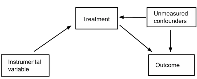
Figure 1: The directed acyclic graph for the relationship between the instrumental variable, treatment, unmeasured confounders and outcome.
measured confounders that affect both the treatment and the outcome. The instrumental variable method is designed to estimate the effects of treatments when there are unmeasured confounders. The method requires a valid instrumental variable which is a variable that (1) is associated with the treatment conditioning on the measured covariates; (2) is independent of the unmeasured confounders conditioning on the measured covariates; (3) has no direct effect on the outcome beyond its effect on the treatment. The definition of an instrumental variable is illustrated in Figure 1, where the arrows represent the causal relationship. The lack of an arrow between the instrumental variable and unmeasured confounding represents assumption (2); The lack of an arrow between the instrumental variable and outcome rep-resents assumption (3). The existence of an arrow between the treatment and instruments represents assumption (1) when the instrumental variable causes the treatment. Note that assumption (1) is also satisfied when the instrumental variable is associated with the treat-ment, but does not cause the treattreat-ment, seeHernan & Robins(2006). SeeHolland (1988),
Angrist et al. (1996), Tan (2006), Cheng et al. (2009), Brookhart et al. (2009), Baiocchi
et al. (2014) and Imbens(2014) for good discussions of instrumental variable methods.
to that of the two stage least square method. In the second stage of the control function method, the outcome is regressed on the treatment, baseline covariates and the residual of the first stage regression and the coefficients of the second stage regression are taken as the control function estimates. Intuitively, the residual of the first stage regression accounts for the unmeasured confounders. The method is called the control function method because the effect of the unmeasured confounders is controlled for via the inclusion of the control function (residual of the first stage regression) in the second stage regression. The control function method has been developed in econometrics (Heckman (1976); Ahn & Powell
(2004); Andrews & Schafgans (1998); Blundell & Powell (2004); Imbens & Wooldridge
(2007)) and also in biostatistics and health services research (Nagelkerke et al (2000) and
Terza et al. (2008)), where the method has been called the two stage residual inclusion
method.
When the treatment has a linear effect on the outcome, then the control function method and two stage least squares produce identical estimates. However, when the treatment has a nonlinear effect on the outcome, then the methods produce different estimates. Settings in which the treatment is thought to have a nonlinear effect on the outcome are common; examples include the effect of the concentration of a drug in a person’s body on the body’s response (Nedelman et al,2007), the effect of education on earnings (Card,1994), the effect of a bank’s financial capital on its costs (Hughes & Mester,1998) and the effect of industry lobbying on government tariff policy (Gawande & Bandyopadhyay ,2000).
Imbens & Wooldridge (2007) conjectured that the control function estimator, while
less robust than two stage least squares, might be much more precise because it keeps the treatment variables in the second stage. However, Imbens and Wooldridge note that a systematic comparison had not been done between the two estimators. The goal of this paper is to provide such a systematic comparison of the control function method to two stage least squares for nonlinear causal effect models.
We illuminate the relationship between control function and two stage least squares estimators by showing that the control function estimator is equivalent to a two stage least squares estimator with an augmented set of instrumental variables. When these augmented instrumental variables are valid, the control function method is more efficient than usual two stage least squares. For example, in the setting (1) of Table 1, the control function estimator is considerably more efficient than two stage least squares, sometimes more than 10 times more efficient. However, when the augmented instrumental variables are invalid, the control function method is inconsistent. Thus, the key issue for deciding whether to use the control function estimator vs. usual two stage least squares is whether the augmented instrumental variables are valid. The validity of the augmented instrumental variables can be tested using the Hausman test (Hausman, 1978). We develop a pretest estimator based on this test and show that it performs well in simulation studies, being close to the control function estimator when the augmented instrumental variables are valid and close to two stage least squares when the augmented instrumental variable are invalid. The pretest estimator combines the strengths of the control function and two stage least squares estimators.
squares with an augmented set of instrumental variables. In section 4, we describe the Hausman test for the validity of the augmented instrumental variables and formulate a pretest estimator. In section 5 , we present simulation studies comparing the control function method to the usual two stage least squares method. In section 6, we apply our methods to a study of the effect of exposure of violence on time preference. In section 7, we present discussions about more generalized models. In section 8, we conclude the paper. The proof of theorems, more simulation studies and two additional data analysis are presented in the Appendix.
2. Set up of model and description of methods
In this section, we introduce the model and describe the control function and the two stage least squares method. In Section 2.1, the model is introduced; In Section 2.2 and 2.3, we describe the two stage least squares method and the control function method, respectively. In Section 2.4, we discuss the assumptions for the control function method.
2.1 Set up of model
In this paper, our focus is on a model where the outcome variable is a non-linear function of the treatment variable. Let y1 denote the outcome variable andy2 denote the treatment variable. Letz1denote a vector of measured pre-treatment covariates andz2 denote a vector of instrumental variables andz = (z1, z2). In the following discussion, we assume both z1 and z2 are one dimensional. In section 3.4, we will extend the method to allow z1 and z2 to be vectors.
For defining the causal effect of the treatment, we use the potential outcome approach
(Rubin(1974) andNeyman(1923)). Let y(y
∗ 2)
1 denote the outcome that would be observed if the unit is assigned treatment level y2 =y∗2. An additive, non-linear causal effect model for the potential outcomes (similar to the linear causal effect model inHolland (1988)) is
y(y ∗ 2)
1 =y (0)
1 +β1g1(y2∗) +β2g2(y∗2) +· · ·+βkgk(y∗2), (1)
where g1(y2∗) = y∗2 and g1,· · · , gk are linearly independent functions. Since g1 is linear,
g2,· · · , gk are non-linear functions. The causal effect of increasing y2 from y∗2 toy2∗+ 1 is
(β1(y2∗+ 1) +β2g2(y2∗+ 1) +· · ·+βkgk(y2∗+ 1))−(β1y ∗
2+β2g2(y ∗
2) +· · ·+βkgk(y2∗)).
We assume that the pretreatment covariate z1 has a linear effect on potential outcomes, E
y(0)1 |z1
=β0+βk+1z1 and denote the residual byu1 =y (0) 1 −E(y
(0)
1 |z1). The model for the observed data is
y1 =β0+β1g1(y2) +β2g2(y2) +· · ·+βkgk(y2) +βk+1z1+u1, (2)
wherey2is the observed value of the treatment variable andg1(y2) =y2.For identifiability, we assume thatgi(0) = 0 for 2≤i≤k. We also assume thaty2’s expectation givenz1 and
z2 is linear in parameters but possibly nonlinear in z1 and z2,i.e.,
whereα2 6=0,z1 andz2 are independent ofu1 andv2,u1 and v2 are potentially correlated, and H = (z2, h2(z2),· · ·, hk(z2)) is a known vector of linearly independent functions of
z2. J is a known vector of functions, which can be a nonlinear function, for simplicity of notation, we will assume a linear effect of z1 henceforth,
y2 =α0+α1z1+αT2H(z2) +v2, (4) We say that I(z2) = (z2, h2(z2)· · · , hk(z2)) are valid instrumental variables if I(z2) satisfies the following two assumptions (Stock (2002), White (1984)(p.8) and Wooldridge
(2010)(p.99)):
Assumption 1 (Relevance)The instruments are correlated with the endogenous variables
W = (g1(y2),· · ·, gk(y2))given z1, that is, E
W I(z2)T|z1
is of full column rank.
Assumption 2 (Exogeneity)The instruments are uncorrelated with the error in(2), that is,
E(I(z2)u1) = 0.
To ensure assumption1, we need to have at leastkvalid instrument variables forg1(y2),· · ·, gk(y2). This requires that the instrument z2 has at least k different values. Otherwise, we cannot constructklinearly independent functions of z2 to be instruments forg1(y2),· · · , gk(y2). Remark 1 In econometric terminology, y2 is called an endogenous variable, z1 are called included exogenous variables and I(z2) = (z2, h2(z2)· · ·, hk(z2)) is called an excluded ex-ogenous variable. Sometimes z1, z2, h2(z2),· · ·, hk(z2) together are referred to as the in-strumental variables (i.e., both the included and excluded exogenous variables), but we will just refer toI(z2) = (z2, h2(z2)· · · , hk(z2))(the excluded exogenous variable) as the instru-ments. Assumption 1 is called the rank condition in the econometric literature while r ≥k is called the order condition. As discussed in Wooldridge(2010)(p.99), the order condition is necessary for the rank condition.
Remark 2 Sufficient conditions for Assumption 2 to hold are that (i) I is independent of the potential outcome y1(0) after controlling for the measured confoundersz1, that is I is independent of unmeasured confounders and (ii)I has no direct effect on y1 and only affects y1 through y2. These conditions are discussed by Holland (1988).
2.2 Description of two stage least squares method
In the following, we will describe the two stage least squares (2SLS) method briefly. Let y ∼ x1+x2 denote linear regression of y on x1, x2 and an intercept. Following Kelejian (1971), the usual two stage least squares estimator is introduced as Algorithm1.
We will refer to this as the usual two stage least squares method as we will show in section 3 that the control function method can be viewed as a two stage least squares method with an augmented set of instruments.
LetL(y|x) denote the best linear projectionγTxofyontoxwhereγ = arg minτE (y−τTx)2
Algorithm 1 Two stage least squares estimator (2SLS)
Input: i.i.d observations of pre-treatment covariates z1, instrumental variables
(z2, h2(z2)· · ·, hk(z2)), the treatment variabley2 and outcome variabley1.
Output: The two stage least squares estimator βb2SLS of treatment effects β = (β1, β2,· · · , βk) in (2).
1: Implement the regression
y2 ∼z1+z2+h2(z2) +· · ·+hk(z2),
.. .
gk(y2)∼z1+z2+h2(z2) +· · ·+hk(z2),
(5)
and obtain the corresponding predicted values as
b
y2,g2(y2),\ · · ·,g\k(y2).
2: Implement the regression:
y1 ∼y2b +· · ·+g\k(y2) +z1. (6)
The two stage least squares estimates are the coefficient estimates on y2, g2(y2),· · · , gk(y2) from (6).
of y1 onto 1, L(g1(y2)|Z),· · ·, L(gk(y2)|Z), z1 is
L(y1|1, L(g1(y2)|Z),· · · , L(gk(y2)|Z), z1) =β0+ k
X
i=1
βiL(gi(y2)|Z) +βk+1z1.
Thus, if we knowL={L(g1(y2)|Z),· · · , L(gk(y2)|Z)}, then the least squares estimate ofy on 1, L(g1(y2)|Z),· · · , L(gk(y2)|Z), z1 will provide an unbiased estimate ofβ. Even though Lis unknown, we can obtain a consistent estimate ofL. Substituting this estimate into the second stage regression provides a consistent estimate ofβ under regularity conditions. See
White (1984)(p21, p32) for the details.
2.3 Description of the control function method
We introduce the control function (CF) method in Algorithm2.
2.4 Additional assumptions of control function
The consistency of control function estimators requires stronger assumptions thanI(z2) sat-isfying Assumptions1and2, that is, stronger thanI(z2) being valid instrumental variables. The control function method is consistent under the following additional assumptions in addition to Assumptions 1and 2 (Imbens & Wooldridge,2007):
Assumption 3 u1 and v2 are independent of z= (z1, z2).
Assumption 4 E(u1|v2) =L(u1|v2) where L(u1|v2) =ρv2 andρ= E(u1v2)
Algorithm 2 Control function estimator (CF)
Input: i.i.d observations of pre-treatment covariates z1, instrumental variables
(z2, h2(z2)· · ·, hk(z2)), the treatment variabley2 and outcome variabley1.
Output: The control function estimator βbCF of treatment effects β = (β1, β2,· · ·, βk) in (2).
1: Implement the regression
y2 ∼z1+z2+h2(z2) +· · ·+hk(z2) (7)
and obtain the predicted valuey2b and the residuale1 =y2−y2.b
2: Implement the regression
y1∼y2+· · ·+gk(y2) +z1+e1. (8)
The control function estimates are the coefficient estimates on y2, g2(y2),· · ·, gk(y2) from the above regression (8).
Remark 3 We only assume z= (z1, I(z2))is uncorrelated with u1 in Assumption 2. Two stage least squares does not make assumptions about v2 but the control function method relies on assumptions about v2. If(u1, v2) follow bivariate normal distribution, Assumption
4 is satisfied automatically.
Model (29) is an example where I(z2) = z2, z22 are valid instrumental variables that satisfy Assumptions1 and 2 but not Assumption 3and 4. The simulation results in Table
1 show that the control function estimate for model (29) is biased.
Assumptions3and4 are sufficient but not necessary conditions for the control function method to be consistent. To investigate the consistency of the control function method, we can express (2) as
y1=β0+β1g1(y2) +β2g2(y2) +· · ·+βkgk(y2) +βk+1z1+ρv1+e, (9)
whereeis u1−ρv2. Under some regularity conditions (Wooldridge (2010) p.56), one suffi-cient condition for the control function method to be consistent is that the new error ein (9) is uncorrelated withgi(y2):
E(gi(y2)e) = 0 for i= 1,· · · , k. (10)
Assumptions 1,2, 3 and 4 lead to E(f(y2)e) = 0 for all f, which is stronger than the sufficient condition (10). In Section 4, we develop a test for the consistency of the control function method that can help to decide whether the control function estimator should be used.
3. Relation between control function and two stage least squares
In this section, we compare the control function and the two stage least squares estimator. To better understand the control function method, we will first focus on the casek= 2
y2 =α0+α1z1+α2z2+α3h2(z2) +v2. For example, a common model has g2(y2) =y22 andh2(z2) =z22.
3.1 Loss of information for the control function method and comparison to two stage least squares
Two stage least squares regressesy1ony2b =LS(y2|1, z1, z2, h2(z2)),g2\(y2) =LS(g2(y2)|1, z1, z2, h2(z2)) and z1 whereLS(A|B) denotes the least square estimate of the linear projection of A onto
span (B). The control function estimator regresses y1 on y2, g2(y2), z1 and e1 = y2−y2.b Intuitively, it seems that the control function method is better than two stage least squares since it keeps y2 and g2(y2) in the second stage regression rather than losing information by replacing y2 and g2(y2) by projections as two stage least squares does. However, the control function method also loses information as explained in the following theorem.
Theorem 1 The following regression
y1∼z1+ye2+g^2(y2),
will have the same estimates of the corresponding coefficients as the second stage regression of the control function method:
y1 ∼z1+y2+g2(y2) +e1,
where e1 is the residual of the regression y2 ∼z1+z2+h2(z2) and ye2 is the residual of the regressiony2 ∼e1 and g^2(y2) is the residual of the regressiong2(y2)∼e1. By the property of OLS, ye2 differs from yˆ2 only by a constant.
Proof In appendix B.
From Theorem 1, the control function method can be viewed as a two stage estimator similar to two stage least squares: in the first stage, the exogenous part of the endogenous variables, ye2 and g^2(y2), are obtained by taking residuals from regressing y2 and g2(y2) on the variable e1 respectively and in the second stage, the endogenous variables in the regression are replaced by the exogenous parts.
Although both the control function method and two stage least squares lose information by projectingg2(y2) andy2to subspaces, the control function method does preserve more in-formation. Let (span{e1})⊥denote the orthogonal complement of the space spanned by the vectore1and span{1, z1, z2, h2(z2)}denote the space spanned by the vectors 1, z1, z2, h2(z2). The control function method projects g2(y2) and y2 to (span{e1})⊥ while two stage least squares projectsg2(y2) andy2to span{1, z1, z2, h2(z2)}, which is a subspace of (span{e1})⊥. We will now show that the control function method is equivalent to two stage least squares with an augmented set of instrumental variables.
3.2 Equivalence of control function to two stage least squares with an augmented set of instrumental variables
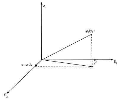
error.iv
g2(y2)
S1
S 2
e1
Figure 2: Projection and Decomposition of the control function Estimator. S1 = span{1, z1, z2, h2(z2)} and S2 = span{error.iv} is defined as the orthogonal complement of S1 in the subspace span{e1}⊥.
is what is the extra part of the control function first stage projection space. The following theorem explains the extra part.
Theorem 2 The following two regressions give the same estimates of corresponding coef-ficients
g2(y2)∼z1+z2+h2(z2) ;
^
g2(y2)∼z1+z2+h2(z2).
Proof In appendix B.
Theorem 2 implies that regressing the control function first stage estimate ofg2(y2),g^2(y2) on {1, z1, z2, h2(z2)} produces the same predicted value for g2(y2) as that of the first stage of two stage least squares. Consequently, the control function method first stage estimate
^
g2(y2) can be decomposed into two orthogonal parts: one part is the same with the two stage least squares first stage estimate and the other part is denoted as error.iv. Letting γ0, γ1, γ2, γ3 denote the coefficients ing2(y2)∼z1+z2+h2(z2), we define
error.iv=g^2(y2)−(γ0+γ1z1+γ2z2+γ3h2(z2)). (11) The decomposition is shown in Figure 2. Let S1 = span{1, z1, z2, h2(z2)} and S2 = span{error.iv}. The projection of g2(y2) to the space S1∪S2 is the control function first
stage predicted valueg2(y2) while the projection of^ g2(y2) to the spaceS1 is the two stage
least squares first stage predicted valueg2(y2). The projection along the direction of\ error.iv
represents the extra part of the control function projection.
Since g^2(y2) is the residual of the regression g2(y2) ∼e1, the first stage regression of control function estimation can be written as
g2(y2) =γc+γe1+g^2(y2)
=γc+γe1+γ0+γ1z1+γ2z2+γ3h2(z2) +error.iv
where the column vector e1 is orthogonal to the column vectors z2, h2(z2), error.iv and error.iv is orthogonal to z1,z2 and h2(z2) by the property of OLS. The following theorem shows the equivalence of the control function estimator to the two stage least squares method with an augmented set of instruments.
Theorem 3 The control function estimator with instrumentsz1, z2, h2(z2)in the first stage is equivalent to the two stage least squares estimator with instrumentsz1, z2, h2(z2), error.iv in the first stage.
Proof In appendix B.
We now show that if Assumptions 3 and 4 do hold, the extra instrument error.iv is a valid instrumental variable, that is, error.iv satisfies Assumptions 1 and 2. Recall the definition e = u1 −ρv2. By Assumptions 3 and 4, E(g2(y2)e) = 0 and the population version oferror.iv is
g2(y2)−L(g2(y2)|v2, z1, z2, h2(z2))
whereL means the linear projection. Since v2 and z1, z2, h2(z2) are uncorrelated withe, E(error.iv×e) =E((g2(y2)−L(g2(y2)|v2, z1, , h2(z2)))e) = 0.
3.3 Equivalence of control function with two stage least squares with augmented instruments for general nonlinear model
In the last section, we showed the equivalence of control function with two stage least squares for k = 2. In this section, we will show the results hold for k≥ 3 and present an algorithm to find the augmented set of instrumental variables for the general model. This will help us understand the control function estimator’s properties since two stage least squares’ properties are well understood (See Remarks 2 and section3.5 below).
We will first considerk= 3 in our general model (2) and then it will be straightforward to generalize to k >3. The model for k= 3 is
y1 =β0+β1y2+β2g2(y2) +β3g3(y2) +β4z1+u1.
LetI ={z2, h2(z2), h3(z2)}be valid instrumental variables for y2, g2(y2), g3(y2). As in the case ofk= 2, we can find the extra instrumenterror.iv1 forg2(y2). If we do the same thing forg3(y2), we will obtain the extra instrumental variable,error.iv2.prime. However, there exists the problem that the error instrumenterror.iv2.primeis not orthogonal toerror.iv1. This will make error.iv2.prime have a non-zero coefficient when we treaterror.iv2.prime as one of the instrumental variables for g2(y2). The non-zero coefficient will lead to the estimate ofg2(y2) being different from what is used in the second stage of control function. To remove the correlation, we do the regression
Theorem 4 If we regress y2 on z1, z2, h2(z2), h3(z2) in the first stage, then the control function estimator is equivalent to two stage least squares with the augmented set of instru-mental variables z1, z2, h2(z2), h3(z2), error.iv1, error.iv2.
Proof In appendix B.
Remark 4 Since the control function method is the same as two stage least squares with an augmented set of instrumental variables, we can calculate the variance of control func-tion estimators with the help of the known variance formula for two stage least squares ( Wooldridge (2010), page 102).
This generalizes to the general k > 3 model. The following is an algorithm to iden-tify the augmented set of instrumental variables for which the control function estima-tor is equivalent to two stage least squares with the augmented set of instrumental vari-ables. Recall that e1 denotes the residual of the regression y2 ∼ z1 +z2 +h2(z2) + h3(z2) and g^i(y2) = resid(gi(y2) ∼ e1). Set the control function projection space S1 = span{z1, z2, h2(z2), h3(z2)} for y2. Regress g^2(y2) on the space S1 to obtain the residual error.iv1 and set the control function projection space S2 = S1⊕span{error.iv1}, where
⊕ denotes the direct sum of two subspaces. For gj(y2), j = 3,· · · , k, regress g^j(y2) on Sj−1 to obtain the extra instrumenterror.ivj, and set the control function projection space
Sj =Sj−1⊕span{error.ivj}. This algorithm will produce the corresponding set of
instru-mental variables for the control function method. Each nonlinear function of endogenous variables will contribute one extra instrumental variable.
We can generalize Theorem 4 to models withk >3.
Theorem 5 If we regress y2 onz1, z2, h2(z2),· · ·, hk(z2) in the first stage, then the
con-trol function estimator is equivalent to two stage least squares with the augmented set of instrumental variables z1, z2, h2(z2),· · ·, hk(z2), error.iv1, error.iv2,· · ·, error.ivk−1.
The proof of Theorem4 applies to this generalized theorem.
3.4 General nonlinear model of multidimensional instruments z2
In this section, we extend our results to allow z1 and z2 to be vectors. In the vector case, the first stage model is extended as
y2 =α0+αT1J(z1) +αT2H(z2) +v2, (13) whereJ is a known vector of functions of z1 and H= (z2, h2(z2),· · · , hk(z2)) is a known vector of linearly independent functions ofz2.
The first stage of two stage least squares is extended as
y2 ∼J(z1) +z2+h2(z2) +· · ·+hk(z2),
.. .
gk(y2)∼J(z1) +z2+h2(z2) +· · ·+hk(z2),
where the notation y ∼ x, where x = (x1,x2,· · ·,xs) denotes linear regression of y on
x1,x2,· · ·,xs and an intercept. From these k first stage regression, we obtain the predicted
values ofkfirst stage regressions asyb2,g\2(y2),· · ·,g\k(y2)
. In the second stage, we do the following regression:
y1∼yb2+· · ·+g\k(y2) +z1. (15)
The first stage of the control function method is
y2 ∼J(z1) +z2+h2(z2) +· · ·+hk(z2);
e1 =y2−y2.b (16)
In the second stage, we do the following linear regression:
y1 ∼y2+· · ·+gk(y2) +z1+e1. (17)
The generalization of Theorem4 and Theorem 5is as follows:
Theorem 6 If we regress y2 on J(z1),z2, h2(z2),· · · , hk(z2) in the first stage, then the control function estimator is equivalent to two stage least squares with the augmented set of instrumental variables J(z1),z2, h2(z2),· · · , hk(z2), error.iv1, error.iv2,· · · , error.ivk−1.
The proof of Theorem4 applies to this generalized theorem.
3.5 Control function bias formula
To ensure consistency of the control function estimation, the Assumptions 1 and 2 of z2, h2(z2),· · · , hk(z2) being valid instruments are not enough and extra assumptions are
needed, such as Assumptions3and 4. We will present a formula for the asymptotic bias of the control function method when the extra assumptions of control function are not satis-fied. Since we have shown that the control function estimator is a two stage least squares estimator with augmented instrumental variables (Sections3.2and3.3), we could make use of the bias formula of two stage least squares with invalid instrumental variables given in
Small (2007).
Let YN denote the vector of the outcome variable y1, WN denote the matrix whose
columns are the endogenous variable y2, g2(y2),· · · , gk(y2), XN denote the matrix whose
columns are the included exogenous variables z1 andZN denote the matrix whose columns
are the instrumental variablesz2, h2(z2),· · ·, hk(z2) forWN. LetCN = [WN, XN] andDN =
[ZN, XN]. In the second stage, we will replaceCN by the first stage predicted valuesdCN =
DN DNTDN
−1
DTNCN. The two stage least squares estimator is
d CN T
d CN
−1 d CN T
YN.
When the instrumental variables are not valid, there exists asymptotic bias for the esti-mator given in the second stage. For the model
y1 =β0+β1g1(y2) +· · ·+βkgk(y2) +βk+1z1+u1 (18) we could write u1 as
whereZ denote the instrumental variables and andu1−LP(u1|Z) is uncorrelated withZ by the property of OLS. Plugging (19) into (18):
y1 =β0+β1y2+β2y22+β3z1+LP(u1|Z) +u1−LP(u1|Z)
y1−LP(u1|Z) =β0+β1y2+β2y22+β3z1+u1−LP(u1|Z) (20) For (20), we could make use of the two stage least squares method with the outcome variable
y1 −LP(u1|Z) to obtain the consistent estimate
d CN T
d CN
−1 d CN T
[YN−LP(UN|ZN)],
whereUN denotes the vector of error u1 in the second stage. Hence a consistent estimator of the asymptotic bias from using the control function method is
d CN
T
d CN
−1 d CN
T
LP(UN|ZN) (21)
The control function bias formula (21) shows that in order for the control function estimator to be asymptotically unbiased, all augmented instruments are required to be un-correlated with the error of the second stage. It is possible that the augmented instruments are correlated with the second stage error even when ZN are valid instrumental variables.
See the simulation study in section 5.3for an example. In Section 4, we develop a test for whether the augmented instruments are correlated with the error of the second stage.
3.6 Comparison between usual two stage least squares and control function In this section, we compare usual two stage least squares (i.e., without any augmented instruments) to the control function method under the assumptions1and2of valid instru-ments and the additional assumptions 3 and 4 of the control function method. Fork= 3, X = (y2, g2(y2), g3(y2)) denote the endogenous variables and Z1= (z1, z2, h2(z2), h3(z2)) denote the instrumental variables. Z2 = (error.iv1, error.iv2) denote the augmented in-struments and Xe = (e1, δ0e1+error.iv1, δ1e1+δ2error.iv1+error.iv2) denote the resid-ual of regressing X on Z1. According to White (1984), the asymptotic variance of a two stage least squares estimator will not increase when adding extra valid instruments and will decrease as long as the extra valid instruments are correlated with the endoge-nous variables given the current instruments. In our setting, adding Z2 to the list of instrumental variables will decrease the asymptotic variance if Z2 is correlated with X.e SinceE(e1×error.iv) = 0, we haveE(error.iv1X) = 0, E(error.ive 21), δ2E(error.iv12)
and E(error.iv2X) = 0,e 0, E(error.iv21)
. Assume
g2(y2) is not a linear combination of 1, e1, z1, z2andh2(z2) almost surely, (22)
we have E(error.iv12) > 0 and E(error.iv1X)e 6= 0 and E(error.iv2X)e 6= 0. Hence, it follows that the control function estimator is strictly better than two stage least squares under the assumptions 1 and 2 of valid instruments, the additional assumptions 3 and 4
1, z1, z2, h2(z2). For example, assuming the first stage model (13) and g2(y2) = y22 and h2(z2) =z22, the functional assumption (22) is automatically satisfied.
We have shown that the control function estimator is equivalent to the two stage least squares estimator with an augmented set of instrumental variables and certain assumptions will make the control function estimator consistent and more efficient than the two stage least squares estimator. Just as we can view the control function estimator as one type of two stage least squares estimator, we can view the usual two stage least squares estimator without the augmented instruments as one type of control function estimator. For k= 3, if we includee1, e2 and e3, which are the residuals of the regressiony2 ∼z1+z2+h2(z2) + h3(z2),g2(y2)∼z1+z2+h2(z2)+h3(z2) andg3(y2)∼z1+z2+h2(z2)+h3(z2) respectively, in the second stage regression, this control function estimator is the same as the usual two stage least squares estimator without the augmented instruments.
4. A pretest estimator
We will explain how to test the validity of the augmented instrumental variables the con-trol function method uses for k = 2; it is straightforward to extend the test to the more general model. Recall the instruments for the usual two stage least squares estimator: Z1 = (1, z1, z2, h2(z2)); As we have shown (Sections 3.2 and 3.3), the control function es-timator is a two-stage eses-timator with the instruments Z = (Z1, error.iv), where error.iv is the augmented instrumental variable. We useβb2SLS to denote the usual two stage least squares estimator with instruments Z1 and use βbCF to denote the two stage least squares estimator with the augmented set of instruments Z. Under the null hypothesis that the augmented instrumental variable error.iv is valid, the two estimators are consistent and
b
βCF is efficient. Under the alternative hypothesis that the augmented instrumental variable error.iv is invalid, βb2SLS is consistent whileβbCF is not consistent.
The Hausman test (Hausman (1978)) provides a test for the validity of the augmented instrumental variableerror.iv. The test statistic H(βbCF,βb2SLS) is defined as
H(βbCF,βb2SLS) =
b
βCF−βb2SLS T h
Cov
b β2SLS
−Cov
b βCF
i− b
βCF−βb2SLS
, (23)
where CovβbCF
and Covβb2SLS
are the covariance matrices of βbCF and βb2SLS and A− denote the Moore-Penrose pseudoinverse. Under the null hypothesis where the augmented instrumenterror.iv is valid, the test statisticH(βbCF,βb2SLS) is asymptotically χ21.
Based on the statistic H(βbCF,βb2SLS), we introduce a pretest estimator in Algorithm3, which uses the control function estimator if there is not evidence that it is inconsistent and otherwise uses the usual two stage least squares estimator.
Algorithm 3 Pretest estimator
Input: i.i.d observations of pre-treatment covariates z1, instrumental variables
(z2, h2(z2)· · ·, hk(z2)), the treatment variabley2, outcome variable y1 and levelα.
Output: The pretest estimator of treatment effectsβ = (β1, β2,· · ·, βk) in (2).
1: Implement Algorithm1 and obtain the estimator βb2SLS and the corresponding covari-ance structureCovβb2SLS
. Implement Algorithm2and obtain the estimatorβbCF and the corresponding covariance structure CovβbCF
.
2: Calculate the test statistic H(βbCF,βb2SLS) as (23) and define the p-value p = Pχ2(1)≥H(βbCF,βb2SLS)
. The level α pretest estimator is defined as
b
βPretest= (
b
βCF ifp > α b
β2SLS ifp≤α . (24)
5. Simulation study
Our simulation study compares the usual two stage least squares (2SLS) estimator, the control function (CF) estimator and the pretest estimator. We will consider several differ-ent model settings where the assumptions of the control function estimator are satisfied, moderately violated (two settings) and drastically violated and we will also investigate the sensitivity of the control function estimator to different joint distributions of errors. The sample size is 10,000 and we implement 10,000 simulations for each setting. We report the winsorized sample mean of the estimators (WMEAN) and the winsorized root mean square error (WRMSE). The non-winsorized sample mean of the estimators (NWEAN) and the non-winsorized root mean square error (NRMSE) are reported in the appendixC. The win-sorized statistics are implemented as setting the 95-100 percentile as the 95-th percentile and the 0-5 percentile as the 5-th percentile and using the winsorized data to calculate the mean and root mean square error. The winsorized statistics are less sensitive to outliers
(Wilcox & Keselman , 2003). The non-winsorized results summarized in the appendix C
have similar patterns as the winsorized results reported in the following discussion. The outcome model that we are considering is
y1=β0+β1z1+β2y2+β3y22+u1; (25) In the following subsections, we will generate y2 according to different models.
5.1 Setting where the assumptions of the control function estimator are satisfied
For the setting where the assumptions of control function estimator are satisfied, the model we consider is:
y1 = 1 +z1+ 10y2+ 10y22+u1; y2 = 1 +1
8z1+ 1 3z2+
1 8z
2 2 +v2;
where z1 ∼ N(0,1) and z2 ∼ N(0,1) and u1 v2 ∼ N 0 0 , 1 0.5 0.5 1 . Setting
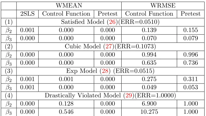
(1) of Table 1 presents the absolute value of ratio of bias of the sample winsorized mean to the true value and the ratio of the sample winsorized root mean square error to the sample winsorized root mean square error of the two stage least squares estimator, where the columns under WMEAN present absolute value of the ratio of the bias and the columns under the WRMSE present the ratio of the root mean square error. Since the ratio of the sample winsorized root mean square error is using the sample winsorized root mean square error of the two stage least squares estimator as the basis, we only report the ratio of the ratio of the sample winsorized root mean square error for the control function estimator and the pretest estimator. ERR represents the empirical rejection rate of the null hypothesis that the extra instrumental variable given by the control function method is valid. The ERR is around 0.05 since the assumptions of CF estimator is satisfied in this model. The usual two stage least squares, control function and pretest estimator all have small bias. The WRMSE of control function estimator is consistently smaller than the WRMSE of the usual two stage least squares estimator. Forβ2 andβ3, the WRMSE are more than 7 times smaller than that of the usual two stage least squares estimator. The pretest estimator also gains substantially over the two stage least squares estimator.
5.2 Setting where the assumptions of the control function estimator are moderately violated
We consider two models where the assumptions of the control function estimator are mod-erately violated,
1. y2 is involved with a cubic function of z2
y1 = 1 +z1+ 10y2+ 10y22+u1; y2 = 1
2×
1 +18z1+13z2+ 18z22+z32
sd 1 +18z1+13z2+ 81z22+z23 +v2;
(27)
where sd 1 +18z1+13z2+18z22+z23is the standard deviation of1+18z1+13z2+18z22+z23 and z1 ∼N(0,1) and z2 ∼N(0,1) and
u1 v2 ∼N 0 0 , 1 0.5 0.5 1 .
2. y2 is involved with an exponential function ofz2.
y1= 1 +z1+ 10y2+ 10y22+u1 y2=
1 2 ×
1 +18z1+13z2+18z22+ exp(z2)
sd 1 + 18z1+ 13z2+81z22+ exp(z2) +v2;
(28)
where sd 1 + 18z1+13z2+18z22+ exp(z2) is the standard deviation of1 +18z1+13z2+ 1
8z 2
2+exp(z2) andz1∼N(0,1) andz2 ∼N(0,1) and u1 v2 ∼N 0 0 , 1 0.5 0.5 1 .
In these simulation settings, since the terms 1 + 18z1 + 13z2 + 18z22 +z23 or 1 + 18z1 + 1
3z2+ 1 8z
2
we standardize these by their standard deviation. The assumptions of the control function estimator are moderately violated in models (27) and (28) since we use a quadratic model of z2 to fit the endogenous variable y2, whose conditional mean has a cubic (exponential) term of z2.
Setting (2) of Table1presents the absolute value of ratio of bias of the sample winsorized mean to the true value of the model (27) and the ratio of the sample winsorized root mean square error to the sample winsorized root mean square error of the two stage least squares estimator. The ratio of bias of two stage least squares, control function and pretest estimator to the true value are small. The empirical rejection rate is around 0.10 and the WRMSE of the control function estimator and the pretest estimator are smaller than WRSME of the two stage least squares estimator.
Setting (3) of Table 1 presents the WMEAN and WRMSE results for the exponential model (28). The ratio of the bias of two stage least squares, control function and pretest estimators to the true value are small. The empirical rejection rate is low and the WRMSE of the control function estimator and the pretest estimator are smaller than WRSME of the two stage least squares estimator. For β3, the WRMSE of the CF estimator and the pretest estimator are around 5% of WRMSE of the usual two stage least squares estimator. Even though the assumption 3 of the control function method is violated for the models (27) and (28), the CF estimator is still approximately unbiased and more efficient than the 2SLS estimator. For these settings, the pretest estimator generally uses the CF estimator and is considerably more efficient than the 2SLS estimator.
5.3 Setting where the assumptions of the control function estimator are drastically violated
We now consider a setting in which the control function assumptions are drastically violated. The model setting is as follows:
y2=−γ2+γ1z2+γ2z22+v2 w=δv22+N(0,1)
y1=β2y2+β3y22+β4w+u1
(29)
where z2 ∼N(0,1) andu1, v2 ∼N
0 0
,
1 0 0 1
and β2 = 1, β3 = 0.2, β4 = 1 and γ1 = 1, γ2 = 0.2 andδ = 0.5.
Setting (4) of Table1presents the absolute value of ratio of bias of the sample winsorized mean to the true value of the model (29) and the ratio of the sample winsorized root mean square error to the sample winsorized root mean square error of the two stage least squares estimator.
WMEAN WRMSE
2SLS Control Function Pretest Control Function Pretest (1) Satisfied Model (26)(ERR=0.0510)
β2 0.001 0.000 0.000 0.139 0.155
β3 0.000 0.000 0.000 0.070 0.079
(2) Cubic Model (27)(ERR=0.1073)
β2 0.000 0.000 0.000 0.994 0.996
β3 0.000 0.000 0.000 0.635 0.736
(3) Exp Model (28) (ERR=0.0515)
β2 0.001 0.001 0.000 0.275 0.311
β3 0.001 0.000 0.000 0.049 0.053
(4) Drastically Violated Model (29)(ERR=1.0000)
β2 0.000 0.128 0.000 6.900 1.000
β3 0.000 0.546 0.000 10.275 1.000
Table 1: The ratio of the bias of the sample winsorized mean (WMEAN) to the true value and the ratio of the Winsorized RMSE (WRMSE) of the control function(Pretest) estimator to WRMSE of the two stage least squares estimator for Satisfied Model (26), Cubic Model (27) with SD = 0.5, Exponential Model (28) with SD = 0.5 and Drastically Violated Model (29). The Empirical Rejection Rate (ERR) stands for the proportion (out of 10,000 simulations) of rejection of the null hypothesis that the extra instrumental variable given by the control function method is valid.
5.4 Sensitivity of joint distribution of errors
In this section, we investigate how sensitive the control function estimator is to different joint distributions of (u1, v2); in particular, we consider settings where Assumption 3 is satisfied but Assumption4 is not satisfied. Assume that we use a quadratic model inz2 to fit the first stage and the true first stage model is quadratic inz2,
y1 = 1 +z1+ 10y2+ 10y22+u1; y2 = 1 +1
8z1+ 1 3z2+
1 8z
2 2 +v2;
(30)
wherez1 ∼N(0,1) andz2∼N(0,1), butu1 and v2 are not bivariate normal. We generate u1 and v2 in the following three ways
1. Double exponential distribution: u1 = 1 and v2 = 121+ √
3
2 2 where 1 and 2 are independent double exponential distribution with mean 0 and variance 1.
2. Bivariate log-normal distribution: u1 = exp (1) and v2 = exp (2) where 1, 2 ∼
N
0 0
,
1 0.5 0.5 1
.
3. Bivariate absolutely normal distribution: u1 =|1| −E|1|andv2 =|2| −E|2|where
1, 2∼N
0 0
,
1 0.5 0.5 1
WMEAN WRMSE
2SLS Control Function Pretest Control Function Pretest (1) Double exponential distribution (ERR=0.0520)
β2 0.001 0.000 0.000 0.154 0.174
β3 0.000 0.000 0.000 0.099 0.112
(2) Log normal distribution(ERR=0.0509)
β2 0.006 0.006 0.006 0.077 0.079
β3 0.001 0.001 0.001 0.060 0.059
(3) Absolute normal distribution(ERR=0.1455)
β2 0.000 0.017 0.011 0.964 1.063
β3 0.000 0.004 0.002 0.968 1.065
Table 2: The ratio of the bias of the sample winsorized mean (WMEAN) to the true value and the ratio of the Winsorized RMSE (WRMSE) of the control function(Pretest) estimator to WRMSE of the two stage least squares estimator for the model (30) and different joint distributions of errors. For this model, the assumption 4of the control function estimator to be consistent is violated.
For these settings, Assumption 3 is satisfied but Assumption 4 is not satisfied. Table
2 presents the ratio of the bias of the sample winsorized mean (WMEAN) to the true value and the ratio of the Winsorized RMSE (WRMSE) of the control function(Pretest) estimator to WRMSE of the two stage least squares estimator for the model (30) and different joint distributions of errors. For the double exponential distribution and the log normal distribution, the ratio of the bias of the usual two stage least squares, the control function and the pretest estimator are small; the WRMSE of the control function and the pretest estimator are much smaller than that of the usual two stage least squares estimator. For the absolute normal distribution, the ratio of the bias of the control function and the pretest estimator are slightly larger than that of the usual two stage least squares; the WRMSE of the control function estimator is slightly smaller than that of the usual two stage least squares estimator and that of the pretest estimator is slightly larger than that of the usual two stage least squares estimator. In summary, the control function estimator is robust to the violations of Assumption 4 considered in this section.
6. Application to a field experiment in Burundi
In this section, we apply the control function method and usual two stage least squares to estimate the effect of exposure to violence on a person’s patience (conflict on time prefer-ence). The data set consists of 302 observations from a field experiment in Burundi (Voors
et al (2012)). Burundi underwent a civil war from 1993-2005, where the intensity of the
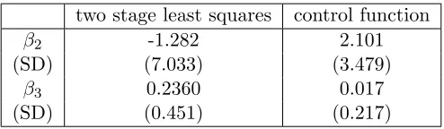
two stage least squares control function
β2 -1.282 2.101
(SD) (7.033) (3.479)
β3 0.2360 0.017
(SD) (0.451) (0.217)
Table 3: Estimates and Standard Error of Coefficients before Endogenous Variables
the person is more patient. The exogenous variables xi that are available are whether the
respondent is literate, the respondent’s age, the respondent’s sex, the total land holding per capita, land Gini coefficient, distance to market, conflict over land, ethnic homogeneity, socioeconomic homogeneity, population density and per capita total expenditure. As dis-cussed inVoors et al (2012), it is possible that the exposure to violence (yi2) is endogenous because violence may be targeted in a non-random way that is related to patience of the community; for example, violence may be targeted to extract “economic profit”, i.e., steal the assets of others, where communities which are more vulnerable to having their assets stolen may also differ in their patience levels from less vulnerable communities. Due to possibility of endogeneity, the OLS estimator of regressing the outcome on the observed covariates maybe a biased estimate of the effect of exposure to violence on time preference. We follow the discussion in the paperVoors et al(2012) and use the following instrumental variables, distance to Bujumbura (the capital of Burundi) and altitude. Fighting was more intense near Bujumbura (the capital of Burundi) and at higher altitudes. The assumption for distance to Bujumbura and altitude to be valid instruments is that they only affect the distribution of violence and are not associated with the patience level of a community.
Voors et al (2012) defend this assumption by discussing that most plausible concern with
its validity is that distance to the capital and altitude might be associated with distance to market which might be associated with patience, but that in Burundi, since most farmers operate at a substance level, selling goods to nearby market, there are local markets in all communities, reducing the possibility of geography being correlated with preference. See more detailed discussion in page 956 inVoors et al(2012). We are able to express our model as
y1i =β0+β1Txi+β2y2i+β3y22i+u,
and
y2i =α0+α1zi1+α2zi2+α3zi21+α4zi22+α5zi1×zi2+α|6xi+v,
wherezi1 represents the distance to Bujumbura andzi2 represents the altitude for thei-th subject.
Table3presents the control function estimate and two stage least squares estimate ofβ2 andβ3. Rather than focus directly onβ2 andβ3, we focus on a more interpretable quantity, the increase of discount rate when percentage dead in attacks increase from y2 to y2+ 1, which we denote byδ(y2),
δ(y2) =yy2+1
1 −y
y2
1 =β2+β3(1 + 2y2).
the point estimate of δ(y2), and the higher curve and lower curve represent the upper and lower bound of 95% confidence interval ofδ(y2) respectively. In Figure3(c), we compare the variance ofδ(y2) provided by control function and usual two stage least squares by plotting the ratio:
V ar.2SLS(δ(y2)) V ar.CF(δ(y2))
,
where V ar.2SLS(δ(y2)) represents the variance of δ(y2) given by usual two stage least squares and V ar.CF(δ(y2)) represents the variance of δ(y2) given by control function. Figure3(c) illustrates that the ratio of variance is always larger than one and shows that the control function estimate is more efficient than the usual two stage least squares estimate. We apply the Hausman test to this real data and the corresponding pvalue is around 0.579 so that the validity of the extra instrumental variable is not rejected and the pretest estimator is equal to the control function estimator.
Figure 3(d) demonstrates the predicted causal relationship between the discount rate and percentage dead in attacks. All the other covariates are set at the sample mean level and we plug in the estimates of the coefficients by the control function method and the two stage least square method. As illustrated, we see that the exposure to violence (measured by percentage dead in attacks) decreases patience (measured by a smaller discount rate).
We present two additional applications of the control function method to estimate the effect of household income on food demand in Appendix D and the effect of smoking during pregnancy on birthweight on Appendix E.
7. Discussion
The model (2) assumes constant treatment effect. The comparison between the CF estima-tor and the 2SLS estimaestima-tor presented in this paper can be extended to more general class of models that allows for heterogeneous treatment effects model, as discussed in section 5 of
Small (2007). Without loss of generality, we consider the outcome model to be a quadratic
model.
y1,i=β0+β1,iy2,i+β2,iy22,i+β3z1,i+u1,i, for i= 1,· · ·, n, (31)
and assume that z2,i and z22,i are valid instruments for y2,i and y22,i. We introduce the
following notation β1=Eβ1,i and β2 =Eβ2,i and assume that
(β1,i, β2,i) is independent of y2,i, z1,i, z2,i, u1,i, (32)
which is a special case of assumption A.3 in Wooldridge (1997) by setting ρ1 = 0. As discussed in Wooldridge (1997) and Small (2007), the assumption (32) states that the units do not select their treatment levels (y2,i andy22,i) based on the gains that they would
experience from the treatment (β1,i and β2,i). The heterogenous effect model (31) can be
expressed as
y1,i =β0+β1y2,i+β2y22,i+β3z1,i+ u1,i+ (β1,i−β1)y2,i+ (β2,i−β2)y22,i
, for i= 1,· · · , n.
The new erroru1,i+ (β1,i−β1)y2,i+ (β2,i−β2)y22,i
has the following property
E u1,i+ (β1,i−β1)y2,i+ (β2,i−β2)y22,i
0 5 10 15
−10
0
10
20
2SLS Estimate of Increase
Percentage dead in attacks
increase of discount r
ate
Upper Point Estimate Lower
0 5 10 15
−10
0
10
20
CF Estimate of Increase
Percentage dead in attacks
increase of discount r
ate
Upper Point Estimate Lower
0 5 10 15
1.0
2.0
3.0
4.0
Ratio of Variance of 2SLS to CF
Percentage dead in attacks
Ratio
0 5 10 15
30
40
50
60
70
80
discount rate prediction
Percentage dead in attacks
discount r
ate
CF 2SLS
where the first part follows from that z1,i is exogenous and the last two part follows from
the assumption (32) . Similarly, we can also show that
E u1,i+ (β1,i−β1)y2,i+ (β2,i−β2)y22,i
z2,i
= 0,
and
E u1,i+ (β1,i−β1)y2,i+ (β2,i−β2)y22,i
z22,i= 0.
Hence, the instrumental variables are valid for the new error. Our theory for the homoge-neous model (2) can be extended to the general (31) under the assumption (32) (it can also be extended under the weaker assumptions than (32) found in Wooldridge (1997)). The pretest estimator provides a consistent estimator and is close to the more efficient estimator between 2SLS and the CF estimator.
We focus on the continuous outcome model in this paper. For a count outcome that follows a log linear model,
logE(y1|y2, z) =β0+β1y2+β2z1+β3u. (33)
where
y=α0+α1z1+α2z2+δ,
andz1 is the included exogenous variable andz2 is the instrumental variable andδis normal variable with zero mean and variance σ2, Mullahy (1997) shows that the 2SLS estimator is inconsistent while the CF estimator is consistent in this count outcome model. For a binary outcome that follows a logistic regression model, comparison of the CF estimator and the 2SLS estimator for the logistic second stage model can be a further research topic, discussion is found inCai et al. (2011) and Clarke & Windmeijer (2012).
Imbens & Rubin (1997) formulated the potential outcome model for binary instrumental
variable and binary treatment, which can be extended to continuous instrumental variable and treatment as follows: The treatmenty2 =fc(z) is an increasing function inzgiven the
compliance classc, wherec∈ {1,· · ·, M}. We also assume the monotonicity assumption of the compliance class
fc0(z)≤fc(z) for c0 ≤c.
The outcome model is
y1|c, z∼N(fc(z) +λc, σ2).
8. Conclusion
This paper compares the control function estimator (Algorithm2) and the usual two stage least squares estimator (Algorithm 1) for nonlinear causal effect models. Theoretically, we show that the control function estimator is equivalent to a two stage least squares estimator with an augmented set of instrumental variables. When the augmented instrumental vari-ables are valid, the control function method will have a larger set of instrumental varivari-ables than the usual two stage least squares estimator and hence the control function estimator will have a smaller variance and root mean square error.
Methodologically, we develop a pretest estimator (Algorithm3) which tests the validity of the augmented instrumental variables and combines the strength of the control function estimator and the usual two sage least squares estimator. In the simulation study, the pretest estimator provides large gains over two stage least squares in some settings while never being much worse than two stage least squares. Such phenomenon is also observed in the real data analysis.
Appendix A. Consistency of the control function estimator
We now investigate why the control function method works under assumptions1,2,3and4. Definee=u1−ρv2. Sinceeis the residual of regressingu1 onv2,eandv2 are uncorrelated. By plugging inu1=e+ρv2, we have
y1 =β0+β1y2+· · ·+βkgk(y2) +βk+1z1+ρv2+e. (34)
Since e is uncorrelated with z1 and v2, it suffices to show that the new error e is un-correlated with gi(y2). By the law of iterated expectation and the one-to-one correspon-dence between y2 and v2, E(gi(y2)e) = E[E(gi(y2)e|y2, z)] = E[gi(y2)E(e|v2, z)]. By
As-sumption 3, E(e|v2, z) = E(u1 −ρv2|v2, z) = E(u1 −ρv2|v2). By Assumption 4, E(u1− ρv2|v2) = E(u1|v2) −ρv2 = 0. Hence, E(gi(y2)e) = 0. and the new error e is uncorre-lated with gi(y2). If we estimate v2 by its estimate ˆv2, the residual of the first stage
y2 ∼z1+z2+h2(z2) +· · ·+hk(z2),the consistency of the control function estimate follows
if we can verify the regularity conditions in Theorem 1 in Murphy et al(2002), which says that if we obtain the consistent estimates of first stage coefficients, we estimate the second stage coefficients consistently by replacing the residual with its estimate from the first stage. LetZdenote the data matrix where each row is an i.i.d sample of{z1, z2, h2(z2),· · ·, hk(z2)}, X denote the data matrix where each row is an i.i.d sample of {z1, y2, g2(y2),· · ·, gk(y2)}
and V2 denote the data matrix where each row is an i.i.d sample of {ˆv2}. The regularity conditions for Theorem 1 inMurphy et al (2002) are the following:
(a) limn→∞ATA=Q0 whereA= (X, V2) andQ0 is positive definite matrix.
(b) v2 = f(α, Z) =y2−(α0+α1z1+α2H(z2)) is twice continuously differentiable inα for each Z and limn→∞ATZ =Q1.
(c) The first stage estimate ˆα is a consistent estimator ofα.
We will show that under the following three regularity assumptions, the conditions (a),(b),(c) of Theorem 1 inMurphy et al (2002) are satisfied.
i limn→∞ATA=Q0 whereA= (X, V2) andQ0 is positive definite matrix.
ii limn→∞ATZ =Q1.
iii The true model of the first stage is (4).
Assumption i is the same as condition (a). Assumption ii is the second part of condition (b). For the first part of condition (b), sincev2=f(α, Z) is a linear function of the parameters α, f is twice continuously differentiable. For condition (c), by assuming iii that the true model of the first stage is (4), the first stage regression coefficients ˆαof the standard control function estimator (7) are consistent estimates ofα.
Appendix B. Proof of the theorems
Lemma 7 (Adjustment Lemma) For the linear model
the following two regression give us the same estimate of β1: y∼x1+x2,
y ∼x1.2; where x1.2 is the residual of the regression x1 ∼x2.
This lemma is called Adjustment Lemma since we adjust x1 tox2 to obtainx1.2.
Proof [Proof of Theorem 1] By the adjustment lemma, the coefficients of the regression y1 ∼z1e+y2e+g2^(y2) are the same with corresponding coefficients iny1∼z1+y2+g2(y2)+e1 wherexeis the residual of the regressionx∼e1. Sincez1is orthogonal toe1by the property of OLS, z1e =z1. The theorem follows by replacing z1e withz1.
Proof[Proof of Theorem 2] LetZ = (1, z1, z2, h2(z2)) denote the matrix of observed values of instrumental variables. y22=γc+γe1+g^2(y2) Since e1 is the residual of the regression
y2∼z1+z2+h2(z2),
it follows from the property of OLS thatZTe1 = 04×1. The coefficients given by regression
g2(y2) ∼ z1+z2+h2(z2) are ZTZ−1ZTg2(y2) and those given by regression g2^(y2) ∼
z1+z2+h2(z2) are ZTZ −1
ZTg^2(y2). Since
ZTZ−1ZTg2(y2)− ZTZ −1
ZTg^2(y2) = ZTZ−1
ZTe1 = 0
we come to the conclusion that the regression g2(y2) ∼ z1 +z2 +h2(z2) and g2^(y2) ∼
z1+z2+h2(z2) give the same estimates of coefficients on 1, z1, z2, h2(z2).
Proof [Proof of Theorem 3] It is sufficient to show that except for a constant difference, (1) y2e is equal to the predicted value of the regression y2 ∼z1+z2+h2(z2) +error.iv.
(2) g2^(y2) is equal to the predicted value of the regression g2(y2) ∼z1+z2+h2(z2) + error.iv.
By the discussion after theorem 2, we have the following decomposition
g2(y2) =γc+γe1+g^2(y2)
=γc+γe1+γ1z1+γ2z2+γ3h2(z2) +error.iv.
(35)
where the column vectore1 is orthogonal to the column vectorsz2, h2(z2) anderror.iv and error.iv is orthogonal toz1, z2 and h2(z2) by the property of OLS. By the decomposition (35), we conclude that except for a constant, g^2(y2) is equal to the predicted value of the
predicted value of the regressiony2 ∼z1+z2+h2(z2) +error.iv is the same withyb2, which is the same with y2.e
Proof [Proof of Theorem 4]
It is sufficient to show that except for a constant difference,
(1) ye2 is equal to the predicted value of the regression
y2∼z1+z2+h2(z2) +h3(z2) +error.iv1+error.iv2.
(2) g2^(y2) is equal to the predicted value of the regression
g2(y2)∼z1+z2+h2(z2) +h3(z2) +error.iv1+error.iv2. (3) g^3(y2) is equal to the predicted value of the regression
g3(y2)∼z1+z2+h2(z2) +h3(z2) +error.iv1+error.iv2.
We start with a decomposition of g3(y2)
g3(y2) =γc+γe1+g^3(y2)
=γc+γe1+γ1z1+γ2z2+γ3h2(z2) +γ4h3(z2) +error.iv2.prime
=γc+γe1+γ1z1+γ2z2+γ3h2(z2) +γ4h3(z2) +γ0error.iv1+error.iv2.
(36)
Since e1 is orthogonal to error.iv1,error.iv2 and z1, z2, h2(z2), h3(z2), the predicted value given by the regressiong3(y2)∼z1+z2+h2(z2) +h3(z2) +error.iv1+error.iv2 is the same withg^3(y2).
Sinceerror.iv2is orthogonal toe1, z1, z2, h2(z2), h3(z2), error.iv1,error.iv2 is orthogonal tog2(y2), hence the coefficient oferror.iv2 given by the following regression
g2(y2)∼z1+z2+h2(z2) +h3(z2) +error.iv1+error.iv2 (37)
is vanishing, which leads to the predicted value of regression (37) is the same with the predicted value of g2(y2)∼z1+z2+h2(z2) +h3(z2) +error.iv1 and by the decomposition (35) and same argument in proof of theorem 3, we obtain (2).
Since error.iv1 and error.iv2 are orthogonal to e1, z1, z2, h2(z2), h3(z2), then error.iv1 and error.iv2 are orthogonal toy2 and (1) follows.
Appendix C. Further results from the simulation study
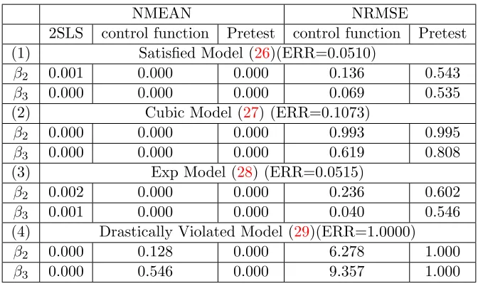
NMEAN NRMSE
2SLS control function Pretest control function Pretest (1) Satisfied Model (26)(ERR=0.0510)
β2 0.001 0.000 0.000 0.136 0.543
β3 0.000 0.000 0.000 0.069 0.535
(2) Cubic Model (27) (ERR=0.1073)
β2 0.000 0.000 0.000 0.993 0.995
β3 0.000 0.000 0.000 0.619 0.808
(3) Exp Model (28) (ERR=0.0515)
β2 0.002 0.000 0.000 0.236 0.602
β3 0.001 0.000 0.000 0.040 0.546
(4) Drastically Violated Model (29)(ERR=1.0000)
β2 0.000 0.128 0.000 6.278 1.000
β3 0.000 0.546 0.000 9.357 1.000
Table 4: The ratio of the bias of the sample non-winsorized mean(NMEAN)to the true value and the ratio of the Non-winsorized RMSE(NRMSE) of the control function(Pretest) estimator to NRMSE of the two stage least squares estimator for Satisfied Model (26), Cubic Model (27) with SD = 0.5, Exponential Model (28) with SD = 0.5 and Drastically Violated Model (29). The Empirical Rejection Rate (ERR) stands for the proportion (out of 10,000 simulations) of rejection of the null hypothesis that the extra instrumental variable given by the control function method is valid.
WMEAN WRMSE
2SLS Control Function Pretest Control Function Pretest (1) Double exponential distribution(ERR=0.0520)
β2 0.001 0.000 0.000 0.150 0.554
β3 0.000 0.000 0.000 0.096 0.546
(2) Log normal distribution(ERR=0.0509)
β2 0.002 0.006 0.009 0.003 0.310
β3 0.000 0.001 0.001 0.002 0.299
(3) Absolute normal distribution(ERR=0.1455)
β2 0.000 0.017 0.010 0.881 1.027
β3 0.000 0.004 0.002 0.883 1.029
two stage least squares control function
β2 39.993 7.389
(SD) ( 22.353) (3.728)
β3 -2.397 1.592
(SD) (2.730) (0.431)
Table 6: Estimates and Standard Error of Coefficients before Endogenous Variables
Appendix D. Application to demand for food
In this section, we apply the control function method and usual two stage least squares to estimate the effect of income on food demand and compare these two methods. The data set is from Bouis & Haddad (1990) and comes from a survey of farm households in the Bukidnon Province of Philippines. FollowingBouis & Haddad (1990), we assume that food expenditure is a quadratic function of log income. Here, y1i is the expenditure on
food of the i-th household, y2i is the log of income of the i-th household and xi represents
the included exogenous variables of the i-th household, which consist of mother’s educa-tion, father’s educaeduca-tion, mother’s age, father’s age, mother’s nutritional knowledge, corn price, rice price , population density of the municipality, number of household members expressed in adult equivalents, and dummy variables for the round of the survey. Then we are able to express our model as y1i = β0 +β1xi +β2y2i+β3y22i +u. Bouis & Haddad
(1990) were concerned that regression of y1 on y2 (log income) and x would not provide an unbiased estimate of β because of unmeasured confounding variables. In particular, because farm households make production and consumption decisions simultaneously and there are multiple incomplete markets in the study area, the households’ production deci-sions (which affect their log income y2) are associated with their preferences according to microeconomic theory (Bardhan & Udry (1999), chap. 2). To solve the problem, Bouis &
Haddad (1990) proposed cultivated area per capita as an instrumental variable. Bouis and
Haddad’s reasoning for why cultivated area per capita is an instrumental variable is that “land availability is assumed to be a constraint in the short run, and therefore exogenous to the household decision making process.”
Table 6 presents the control function estimate and two stage least squares estimate of β2 and β3. Rather than focus directly on β2 and β3, we focus on a more interpretable quantity, the income elasticity of food demand at the mean level of food expenditure. This is the percent change in food expenditure caused by a 1% increase in income for households currently spending at the mean food expenditure level, and we denote it by η(y2). The mean food expenditure of households is 31.14 pesos per capita per week and
η(y2) = 100 31.14
ˆ
β2log(1.01) + ˆβ3 2 log(1.01)y2+ log(1.01)2.
0 1 2 3 4 5 6 −40 −20 0 20 40 60
OLS Estimate of Increase
ln(income)
F
ood Expenditure Increase
Upper Point Estimate Lower
0 1 2 3 4 5 6
−40 −20 0 20 40 60
2SLS Estimate of Increase
ln(income)
F
ood Expenditure Increase
Upper Bound of CI Point Estimate of Increase Lower Bound of CI
0 1 2 3 4 5 6
−40 −20 0 20 40 60
CF Estimate of Increase
ln(income)
F
ood Expenditure Increase
Upper Bound of CI Point Estimate of Increase Lower Bound of CI
0 1 2 3 4 5 6
0 5 10 15 20 25 30 35
Ratio of Variance of 2SLS to CF
ln(income)
Ratio
Figure 4: (a) plots the OLS estimate and 95% confidence interval for the income elasticity with respect to different log(income);(b) plots the two stage least squares estimate and 95% confidence interval for the income elasticity with respect to different log(income);(c) plots the control function estimate and 95% confidence interval for the income elasticity with respect to different log(income);(d) plots the ratio of the variance of two stage least squares to the variance of the control function method with respect to different log(income).
of η(y2) respectively. In Figure4(d), we compare the variance ofη(y2) provided by control function and usual two stage least squares by plotting the ratio:
V ar.2SLS(η(y2)) V ar.CF(η(y2)) ,
where V ar.2SLS(η(y2)) represents the variance of η(y2) given by usual two stage least squares and V ar.CF(η(y2)) represents the variance of η(y2) given by control function. Figure4(b) shows that two stage least squares leads to negative estimate of the non-negative valued Income Elasticity of Food Demand; in contrast, Figure 4(c) shows that the control function estimate of the non-negative valued Income Elasticity of Food Demand is always positive. Figure 4(d) illustrates that the ratio of variance is always larger than one and shows that the control function estimate is more efficient than the usual two stage least squares estimate. We apply the Hausman test to this real data and the corresponding pvalue is around 0.14 so that the validity of the extra instrumental variables is not rejected and the pretest estimator is equal to the control function estimator.
Appendix E. Application to smoking data
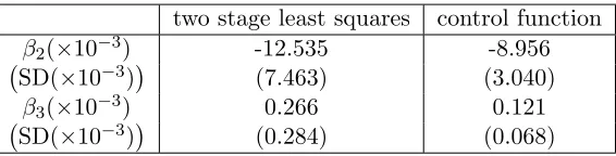
two stage least squares control function
β2(×10−3) -12.535 -8.956
SD(×10−3) (7.463) (3.040)
β3(×10−3) 0.266 0.121
SD(×10−3) (0.284) (0.068)
Table 7: Estimates and Standard Error of Coefficients before Endogenous Variables
Interview Survey. The goal is to estimate the effect of maternal smoking (during pregnancy) on the birth weight. For thei-th observation, the outcomeyi1represents the log birth weight, yi2 represents the typical number of cigarettes smoked per day during pregnancy and xi
represents the other exogenous variables: birth order, race and child’s sex. As discussed
inWehby et al. (2011), it is possible that mothers who smoke during pregnancy self-select
into smoking based on their preferences for health and risk taking and their perceptions of fetal health endowments. These factors, which are typically unobserved in available data samples, can affect the fetal health through other pathways besides smoking. For example, women smoking during pregnancy might adopt other unhealthy behaviors having adverse effects on the fetus (e.g., poorer nutrition or reduced prenatal care). Since some of the confounding variables that are related with both smoking and child health are unobserved, the OLS estimator of regressing the outcome on the observed covariates maybe a biased estimate of the effect of smoking on the birth weight. We follow the discussion in the paperMullahy (1997) and use the following instrumental variables zi: maternal schooling,
paternal schooling, family income and the per-pack state excise tax on the cigarettes. Then we are able to express our model as
y1i =β0+β1Txi+β2y2i+β3y22i+u,
and
y2i =αTzi+v.
Table7presents the control function estimate and two stage least squares estimate ofβ2 andβ3. Rather than focus directly onβ2 andβ3, we focus on a more interpretable quantity, the increase of log birthweight when the cigarettes increase from y2 to y2 + 1, which we denote byδ(y2),
δ(y2) =yy2+1
1 −y
y2
1 =β2+β3(1 + 2y2).
In Figure 5(a)/(b), we plot usual two stage least squares/control function point estimates and corresponding confidence intervals of δ(y2) respectively. The middle curve represents the point estimate of δ(y2), and the higher curve and lower curve represent the upper and lower bound of 95% confidence interval ofδ(y2) respectively. In Figure5(c), we compare the variance ofδ(y2) provided by control function and usual two stage least squares by plotting the ratio:
V ar.2SLS(δ(y2)) V ar.CF(δ(y2))
,