Minimum Density Hyperplanes
Nicos G. Pavlidis [email protected]
Department of Management Science Lancaster University
Lancaster, LA1 4YX, UK
David P. Hofmeyr [email protected]
Department of Mathematics and Statistics Lancaster University
Lancaster, LA1 4YF, UK
Sotiris K. Tasoulis [email protected]
Department of Applied Mathematics Liverpool John Moores University, Liverpool, L3 3AF, UK
Editor:Andreas Krause
Abstract
Associating distinct groups of objects (clusters) with contiguous regions of high prob-ability density (high-density clusters), is central to many statistical and machine learning approaches to the classification of unlabelled data. We propose a novel hyperplane classifier for clustering and semi-supervised classification which is motivated by this objective. The proposed minimum density hyperplane minimises the integral of the empirical probabil-ity densprobabil-ity function along it, thereby avoiding intersection with high densprobabil-ity clusters. We show that the minimum density and the maximum margin hyperplanes are asymptotically equivalent, thus linking this approach to maximum margin clustering and semi-supervised support vector classifiers. We propose a projection pursuit formulation of the associated optimisation problem which allows us to find minimum density hyperplanes efficiently in practice, and evaluate its performance on a range of benchmark data sets. The proposed approach is found to be very competitive with state of the art methods for clustering and semi-supervised classification.
Keywords: low-density separation, high-density clusters, clustering, semi-supervised classification, projection pursuit
1. Introduction
We study the fundamental learning problem: Given a random sample from an unknown probability distribution with no, or partial label information, identify a separating hyperplane that avoids splitting any of the distinct groups (clusters) present in the sample. We adopt the cluster definition given by Hartigan (1975, chap. 11), in which a high-density cluster
is defined as a maximally connected component of the level set of the probability density function, p(x), at level c>0,
levcp(x) =
n
x∈Rdp(x)> c o
An important advantage of this approach over other methods is that it is well founded from a statistical perspective, in the sense that a well-defined population quantity is being estimated.
However, since p(x) is typically unknown, detecting high-density clusters necessarily involves estimates of this function, and standard approaches to nonparametric density es-timation are reliable only in low dimensions. A number of existing density clustering al-gorithms approximate the level sets of the empirical density through a union of spheres around points whose estimated density exceeds a user-defined threshold (Walther, 1997; Cuevas et al., 2000, 2001; Rinaldo and Wasserman, 2010). The choice of this threshold affects both the shape and number of detected clusters, while an appropriate threshold is typically not known in advance. The performance of these methods deteriorates sharply as dimensionality increases, unless the clusters are assumed to be clearly discernible (Rinaldo and Wasserman, 2010). An alternative is to consider the more specific problem of allocating observations to clusters, which shifts the focus to local properties of the density, rather than its global approximation. The central idea underlying such methods is that if a pair of ob-servations belong to the same cluster they must be connected through a path traversing only high-density regions. Graph theory is a natural choice to address this type of problem. Az-zalini and Torelli (2007); Stuetzle and Nugent (2010) and Menardi and AzAz-zalini (2014) have recently proposed algorithms based on this approach. Even these approaches however are limited to problems of low dimensionality by the standards of current applications (Menardi and Azzalini, 2014).
An equivalent formulation of the density clustering problem is to assume that clusters are separated through contiguous regions of low probability density; known as the low-density separation assumption. In both clustering and semi-supervised classification, identifying the hyperplane with the maximum margin is considered a direct implementation of the low-density separation approach. Motivated by the success of support vector machines (SVMs) in classification, maximum margin clustering (MMC) (Xu et al., 2004), seeks the maximum margin hyperplane to perform a binary partition (bi-partition) of unlabelled data. MMC can be equivalently viewed as seeking the binary labelling of the data sample that will maximise the margin of an SVM estimated using the assigned labels.
Encouraging theoretical results for semi-supervised classification have been obtained un-der the cluster assumption. If p(x) is a mixture of class conditional distributions, Castelli and Cover (1995, 1996) have shown that the generalisation error will be reduced exponen-tially in the number of labelled examples if the mixture is identifiable. More recently, Singh et al. (2009) showed that the mixture components can be identified ifp(x) is a mixture of a finite number of smooth density functions, and the separation between mixture components is large. Rigollet (2007) considers the cluster assumption in a nonparametric setting, that is in terms of density level sets, and shows that the generalisation error of a semi-supervised classifier decreases exponentially given a sufficiently large number of unlabelled data. How-ever, the cluster assumption is difficult to verify with a limited number of labelled examples. Furthermore, the algorithms proposed by Rigollet (2007) and Singh et al. (2009) are difficult to implement efficiently even if the cluster assumption holds. This renders them impractical for real-world problems (Ji et al., 2012).
Although intuitive, the claim that maximising the margin over (labelled and) unlabelled data is equivalent to identifying the hyperplane that goes through regions with the lowest possible probability density has received surprisingly little attention. The work of Ben-David et al. (2009) is the only attempt we are aware of to theoretically investigate this claim. Ben-David et al. (2009) quantify the notion of a low-density separator by defining the density on a hyperplane, as the integral of the probability density function along the hyperplane. They study the existence of universally consistent algorithms to compute the hyperplane with minimum density. The maximum hard margin classifier is shown to be consistent only in one dimensional problems. In higher dimensions only a soft-margin algorithm is a consistent estimator of the minimum density hyperplane. Ben-David et al. (2009) do not provide an algorithm to compute low density hyperplanes.
This paper introduces a novel approach to clustering and semi-supervised classification which directly identifies low-density hyperplanes in the finite sample setting. In this ap-proach the density on a hyperplane criterion proposed by Ben-David et al. (2009) is directly minimised with respect to a kernel density estimator that employs isotropic Gaussian ker-nels. The density on a hyperplane provides a uniform upper bound on the value of the empirical density at points that belong to the hyperplane. This bound is tight and propor-tional to the density on the hyperplane. Therefore, the smallest upper bound on the value of the empirical density on a hyperplane is achieved by hyperplanes that minimise the den-sity on a hyperplane criterion. An important feature of the proposed approach is that the density on a hyperplane can be evaluated exactly through a one-dimensional kernel density estimator, constructed from the projections of the data sample onto the vector normal to the hyperplane. This renders the computation of minimum density hyperplanes tractable even in high dimensional applications.
We establish a connection between the minimum density hyperplane and the maximum margin hyperplane in the finite sample setting. In particular, as the bandwidth of the kernel density estimator is reduced towards zero, the minimum density hyperplane converges to the maximum margin hyperplane. An intermediate result establishes that there exists a positive bandwidth such that the partition of the data sample induced by the minimum density hyperplane is identical to that of the maximum margin hyperplane.
establishes the connection between minimum density hyperplanes and maximum margin hyperplanes. Section 4 discusses the estimation of minimum density hyperplanes and the computational complexity of the resulting algorithm. Experimental results are presented in Section 5, followed by concluding remarks and future research directions in Section 6.
2. Problem Formulation
We study the problem of estimating a hyperplane to partition a finite data set, X =
{xi}ni=1⊂Rd, without splitting any of the high-density clusters present. We assume thatX is an i.i.d. sample of a random variableXonRd, with unknown probability density function
p : Rd → R+. A hyperplane is defined as H(v, b) := {x ∈ Rd|v·x = b}, where without loss of generality we restrict attention to hyperplanes with unit normal vector, i.e., those parameterised by (v, b) ∈ Sd−1 ×
R, where Sd−1 = {v ∈ Rdkvk = 1}. Following Ben-David et al. (2009) we define the density on the hyperplane H(v, b) as the integral of the probability density function along the hyperplane,
I(v, b) := Z
H(v,b)
p(x)dx. (1)
We approximatep(x) through a kernel density estimator with isotropic Gaussian kernels,
ˆ
p(x|X, h2I) = 1
n(2πh2)d/2
n
X
i=1
exp
−kx−xik
2 2h2
. (2)
This class of kernel density estimators has the useful property that the integral in Equa-tion (1) can be evaluated exactly by projecting X onto v; constructing a one-dimensional density estimator with Gaussian kernels and bandwidthh; and evaluating the density atb,
ˆ
I(v, b|X, h2I) := Z
H(v,b)
ˆ
p x|X, h2Idx,
= 1
n
√
2πh2
n
X
i=1
exp
−(b−v·xi)
2 2h2
= ˆp b| {v·xi}ni=1, h2
. (3)
The univariate kernel estimator ˆp · | {v·xi}ni=1, h2
approximates the projected density on v, that is, the density function of the random variable, Xv = X·v. Henceforth we
use ˆI(v, b) to approximate I(v, b). To simplify terminology we refer to ˆI(v, b) as the den-sity on H(v, b), or the density integral on H(v, b), rather than the empirical density, or the empirical density integral, respectively. For notational convenience we write ˆI(v, b) for
ˆ
I(v, b|X, h2I), where X and h are apparent from context.
The following Lemma, adapted from (Tasoulis et al., 2010, Lemma 3), shows that ˆI(v, b) provides an upper bound for the maximum value of the empirical density at any point that belongs to the hyperplane.
Lemma 1 Let X = {xi}ni=1 ⊂ Rd, and pˆ(x|X, h2I) be a kernel density estimator with
isotropic Gaussian kernels. Then, for any (v, b)∈ Sd−1× R,
max
x∈H(v,b)pˆ(x
|X, h2I)6 2πh2
1−d
This lemma shows that a hyperplane, H(v, b), cannot intersect level sets of the empirical
density with level higher than 2πh21−2d ˆ
I(v, b). The proof of the lemma relies on the fact that projection contracts distances, and follows from simple algebra. In Equation (4) equality holds if and only if there exists x ∈ H(v, b) and c ∈ Rn such that all x
i ∈ X,
can be written as xi = x+civ. It is therefore not possible to obtain a uniform upper
bound on the value of the empirical density at points that belong to H(v, b) that is lower
than 2πh2
1−d
2 Iˆ(v, b) using only one-dimensional projections. Since the upper bound of
Lemma 1 is tight and proportional to ˆI(v, b), minimising the density on the hyperplane leads to the lowest upper bound on the maximum value of the empirical density along the hyperplane separator.
To obtain hyperplane separators that are meaningful for clustering and semi-supervised classification, it is necessary to constrain the set of feasible solutions, because the density on a hyperplane can be made arbitrarily low by considering a hyperplane that intersects only the tail of the density. In other words, for any v, ˆI(v, b) can be made arbitrarily low for sufficiently large |b|. In both problems the constraints restrict the feasible set to a subset of the hyperplanes that intersect the interior of the convex hull ofX. In detail, let convX denote the convex hull of X, and assume Int(convX)6= ∅. DefineC to be the set of hyperplanes that intersect Int(convX),
C =nH(v, b)
(v, b)∈ S
d−1×
R,∃z∈Int(convX) s.t. v·z=b
o
. (5)
Then denote byF the set of feasible hyperplanes, where F ⊂C. We define the minimum density hyperplane(MDH), H(v?, b?)∈F to satisfy,
ˆ
I(v?, b?) = min (v,b)|H(v,b)∈F
ˆ
I(v, b). (6)
In the following subsections we discuss the specific formulations for clustering and semi-supervised classification in turn.
2.1 Clustering
Since high-density clusters are formed around the modes of p(x), the convex hull of these modes would be a natural choice to define the set of feasible hyperplanes. Unfortunately, this convex hull is unknown and difficult to estimate. We instead propose to constrain the distance of hyperplanes to the origin, b. Such a constraint is inevitable as for any v ∈ Sd−1, ˆI(v, b) can become arbitrarily close to zero for sufficiently large |b|. Obviously, such hyperplanes are inappropriate for the purposes of bi-partitioning as they assign all the data to the same partition. Rather than fixing b to a constant, we constrain it in the interval,
F(v) = [µv−ασv, µv+ασv], (7)
where µv and σv denote the mean and standard deviation, respectively, of the projections {v·xi}ni=1. The parameterα>0, controls the width of the interval, and has a probabilistic
few outlying observations. We discuss in detail how to set this parameter in the experimen-tal results section. If Int(convX)6=∅, then there exists α >0 such that the set of feasible hyperplanes for clustering, FCL, satisfies,
FCL= n
H(v, b)
(v, b)∈ S
d−1×
R, b∈F(v)
o
⊂C, (8)
whereC is the set of hyperplanes that intersect Int(convX), as defined in Equation (5). The minimum density hyperplane for clustering is the solution to the following con-strained optimisation problem,
min (v,b)∈Sd−1×
R
ˆ
I(v, b), (9a)
subject to: b−µv+ασv>0, (9b)
µv+ασv−b>0. (9c)
Since the objective function and the constraints are continuously differentiable, MDHs can be estimated through constrained optimisation methods like sequential quadratic program-ming (SQP). Unfortunately the problem of local minima due to the nonconvexity of the objective function seriously hinders the effectiveness of this approach.
To mitigate this we propose a parameterised optimisation formulation, which gives rise to a projection pursuit approach. Projection pursuit methods optimise a measure of “inter-estingness” of a linear projection of a data sample, known as the projection index. For our problem the natural choice of projection index forvis the minimum value of the projected density within the feasible region, minb∈F(v)Iˆ(v, b). This index gives the minimum density integral of feasible hyperplanes with normal vector v. To ensure the differentiability of the projection index we incorporate a penalty term into the objective function. We define the penalised density integral as,
fCL(v, b) = ˆI(v, b) +
L
η max{0, µv−ασv−b, b−µv−ασv}
1+, (10)
where, L = e1/2h2√2π−1
> supb∈R
∂Iˆ(v,b)
∂b
, ∈ (0,1) is a constant term that ensures that the penalty function is everywhere continuously differentiable, and η ∈ (0,1). Other penalty functions are possible, but we only consider the above due to its simplicity, and the fact that its parameters offer a direct interpretation: Lin terms of the derivative of the projected density onv; andηin terms of the desired accuracy of the minimisers offCL(v, b) relative to the minimisers of Equation (9), as discussed in the following proposition.
Proposition 2 For v∈ Sd−1, define, the set of minimisers,
B(v) = arg min
b∈F(v)
ˆ
I(v, b), (11)
BC(v) = arg min
b∈R
fCL(v, b) (12)
For every b? ∈B(v) there exists b?C ∈BC(v) such that |b?−b?C|6η. Moreover, there are
no minimisers of fCL(v, b) outside the interval [µv−ασv−η, µv+ασv+η],
Proof
Any minimiser in the interior of the feasible region,b? ∈B(v)∩Int(F(v)), also minimises the penalised function, sincefCL(v, b) = ˆI(v, b) for allb∈Int(F(v)), henceb? ∈BC(v).
Next we consider the case when either or both of the boundary points ofF(v),b−=µv−
ασvandb+=µv+ασv, are contained inB(v). It suffices to show that,fCL(v, b)>Iˆ(v, b−)
for all b < b−−η, and fCL(v, b) > Iˆ(v, b+) for all b > b++η. We discuss only the case
b > b++η as the treatment ofb < b−−η is identical. Assume that ˆI(v, b)<Iˆ(v, b+) (since in the opposite case the result follows immediately: fCL(v, b) >Iˆ(v, b)>Iˆ(v, b+)). From the mean value theorem there exists ξ∈(b+, b) such that,
ˆ
I(v, b+) = ˆI(v, b)−(b−b+) ∂Iˆ(v, b)
∂b
b=ξ
6Iˆ(v, b) + (b−b+)L <Iˆ(v, b) +L(b−b
+)1+
η =fCL(v, b).
In the above we used the following facts: ∂Iˆ(∂bv,b)
b=ξ<0,L>supb∈R
∂Iˆ(v,b)
∂b
, and
b−b+
η >1.
We define the projection index for the clustering problem as the minimum of the pe-nalised density integral,
φCL(v) = min
b∈R
fCL(v, b). (13)
Since the optimisation problem of Equation (13) is one-dimensional it is simple to compute the set of global minimisersBC(v). As we discuss in Section 4, this is necessary to compute
directional derivatives of the projection index, as well as, to determine whetherφCL is dif-ferentiable. We call the optimisation ofφCL,minimum density projection pursuit(MDP2). For each v, MDP2 considers only the optimal choice of b. This enables it to avoid local minima of ˆI(v,·). Most importantly MDP2 is able to accommodate a discontinuous change in the location of the global minimiser(s), arg minb∈RfCL(v, b), as v changes. Neither of the above can be achieved when the optimisation is jointly over (v, b) as in the original constrained optimisation problem, Equation (9). The projection index φCL is continuous, but it is not guaranteed to be everywhere differentiable whenBC(v) is not a singleton. The
resulting optimisation problem is therefore nonsmooth and nonconvex.
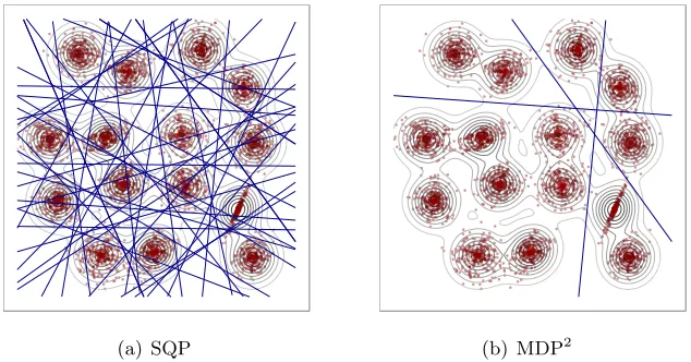
(a) SQP (b) MDP2
Figure 1: Binary partitions induced by 100 MDHs estimated through SQP and MDP2
● ● ● ● ● ● ● ● ● ●● ●●●●●●●● ●●●●●● ● ● ● ● ● ● ● ● ● ● ● ●● ●●●●●●●● ● ● ● ● ● ● ● ● ● ● ● ● ●●●●●●●●● ●●● ●● ● ● ● ● ● ● ● ● ● ● ● ●● ● ● ● ● ● ● ● ● ● ● ●●●●●●●●●●●● ●●●●●● ●●●●● ● ● ● ● ● ● ● ● ● ● ● ● ● ● ● ● ● ● ● ● ● ● ● ● ● ● ● ●●●●●●●●●●● ●● ● ● ● ● ● ● ● ● ● ●● ● ● ● ● ● ● ● ● ●●●●●●●● ● ●●●●● ● ● ● ● ● ● ● ● ● ● ● ●● ●●●●●●●●●●●●●●●●●●● ●●●● ●●● ●●● ●● ●●● ●●● ●●●●●●●●●● ●●●● ● ● ● ● ● ●●●●●●●●●●●●●●●●●●● ●● ● ●● ● ● ● ● ● ● ● ● ● ● ● ● ● ● ● ● ● ●●●●●●●●● ● ● ● ● ●
Projection Index: φCL(θ)
0.06
0.10
0.14
0.18
0 π4 π2 3π4 π
Projection Angle: θ
SQP
MDP2
0 π4 π2 3π4 π
0 10 20 30 40 50
Figure 2: Projection index for S1 data set and solutions obtained through SQP and MDP2
optimal value ofbfor any v(θ) and this indeed occurs in this example. Therefore the value ofφCL(v) is a lower bound for the function values of the minimisers identified through SQP. 2.2 Semi-Supervised Classification
In semi-supervised classification labels are available for a subset of the data sample. The resulting classifier needs to predict as accurately as possible the labelled examples, while avoiding intersection with high-density regions of the empirical density. The MDH formula-tion can readily accommodate partially labelled data by incorporating the linear constraints associated with the labelled data into the clustering formulation. Without loss of generality assume that the first ` examples are labelled by y = (y1, . . . , y`)> ∈ {−1,1}`. The MDH
for semi-supervised classification is the solution to the problem,
min (v,b)∈Sd−1×
R
ˆ
I(v, b), (14a)
subject to: yi(v·xi−b)>0, ∀i= 1, . . . , `, (14b)
b−µv+ασv >0, (14c)
µv+ασv−b>0, (14d)
where ˆI(v, b), µv, and σv are computed over the entire data set. If the labelled examples
are linearly separable the constraints in Equation (14) define a nonempty feasible set of hyperplanes,
FLB= n
H(v, b)|(v, b)∈ Sd−1×R, b∈F(v), yi(v·xi−b)>0, ∀i∈ {1, . . . , l}
o
⊂C.
(15) Equations (14c) and (14d) act as a balancing constraint which discourages MDHs that classify the vast majority of unlabelled data to a single class. Balancing constraints are included in the estimation of S3VMs for the same reason (Joachims, 1999; Chapelle and Zien, 2005).
As in the case of clustering, the direct minimisation of Equation (14) frequently leads to locally optimal solutions. To mitigate this we again propose a projection pursuit formu-lation. We define the penalised density integral for semi-supervised classification as,
fSSC(v, b) =fCL(v, b) +γ
l
X
i=1
max{0,−yi(v·xi−b)}1+ (16)
where, γ >0 is a user-defined constant, which controls the trade-off between reducing the density on the hyperplane, and misclassifying the labelled examples. The projection index is then defined as the minimum of the penalised density integral,
φSSC(v) = min
b∈R
fSSC(v, b). (17)
3. Connection to Maximum Margin Hyperplanes
defined as the minimum Euclidean distance between the hyperplane and its nearest datum,
marginH(v, b) = min
x∈X|v·x−b|. (18)
The points whose distance to the hyperplaneH(v, b) is equal to the margin of the hyper-plane, that is, arg minx∈X|v·x−b|,are called thesupport pointsofH(v, b). LetF denote the set of feasible hyperplanes; then themaximum margin hyperplane(MMH),H(vm, bm)∈F
satisfies,
marginH(vm, bm) = max
(v,b)|H(v,b)∈FmarginH(v, b). (19)
The main result of this section is Theorem 5, which states that as the bandwidth pa-rameter, h, is reduced to zero the MDH converges to the MMH. An intermediate result, Lemma 4, shows that there exists a positive bandwidth,h0 >0 such that, for allh∈(0, h0), the partition of the data set induced by the MDH is identical to that of the MMH.
We first discuss some assumptions which allow us to present the theoretical results of this section. As before we assume a fixed and finite data set X ⊂ Rd, and approximate
its (assumed) underlying probability density function via a kernel density estimator using Gaussian kernels with isotropic bandwidth matrix h2I. We assume that the interior of the convex hull of the data, Int(convX), is non-empty, and define C as the set of hyperplanes that intersect Int(conv X), as in Equation (5). The set of feasible hyperplanes, F, for either clustering or the semi-supervised classification satisfies F ⊂ C. By construction every H(v, b) ∈ F defines a hyperplane which partitions X into two non-empty subsets. Observe that if for each v ∈ Sd−1 the set {b ∈
R|H(v, b) ∈ F} is compact, then by the compactness of Sd−1 a maximum margin hyperplane in F exists. For both the clustering and semi-supervised classification problems this compactness holds by construction.
For any h > 0, let (v?h, b?h) ∈ Sd−1×
R parameterise a hyperplane which achieves the minimal density integral over all hyperplanes inF, for bandwidth matrixh2I. That is,
ˆ
I(vh?, b?h) = min (v,b)|H(v,b)∈F
ˆ
I(v, b). (20)
Following the approach of Tong and Koller (2000) we first show that as the bandwidth, h, is reduced towards zero, the density on a hyperplane is dominated by its nearest point. This is achieved by establishing that for all sufficiently small values ofh, a hyperplane with non-zero margin has lower density integral than any other hyperplane with smaller margin.
Lemma 3 Take H(v, b) ∈F with non-zero margin and 0 < δ < marginH(v, b) := Mv,b.
Then ∃h0 > 0 such that h ∈ (0, h0) and Mw,c := marginH(w, c) 6 Mv,b − δ implies
ˆ
I(v, b)<Iˆ(w, c).
Proof
Using Equation (3) it is easy to see that,
ˆ
I(v, b)6 1
h√2πexp (
−M
2
v,b
2h2 )
,
infnIˆ(w, c)|Mw,c6Mv,b−δ
o
> 1
nh√2π exp
−(Mv,b−δ)
2 2h2
Therefore,
06 lim
h→0+
ˆ
I(v, b)
inf n
ˆ
I(w, c)|Mw,c6Mv,b−δ
o 6 lim
h→0+
nexp
−M
2
v,b
2h2
exp n
−(Mv,b−δ)2
2h2
o = 0.
Therefore, ∃h0>0 such thath∈(0, h0)⇒ Iˆ(v,b)
infnIˆ(w,c)Mw,c6Mv,b−δ
o <1.
An immediate corollary of Lemma 3 is that as h tends to zero the margin of the MDH tends to the maximum margin. However, this does not necessarily ensure the stronger result that the sequence of MDHs converges to the MMH. To establish this we require two technical results, which describe some algebraic properties of the MMH, and are provided as part of the proof of Theorem 5 which is given in Appendix A.
The next lemma uses the previous result to show that there exists a positive bandwidth,
h0 >0, such that an MDH estimated using h ∈(0, h0) induces the same partition of X as the MMH. The result assumes that the MMH is unique. Notice that if X is a sample of realisations of a continuous random variable then this uniqueness holds with probability 1.
Lemma 4 Suppose there is a unique hyperplane inF with maximum margin, which can be parameterised by (vm, bm)∈ Sd−1×
R. Then ∃h0 >0 s.t. h ∈(0, h0) ⇒ H(v?h, b?h) induces
the same partition of X as H(vm, bm).
Proof
Let M = marginH(vm, bm), and letP be the collection of hyperplanes that induce the
same partition of X as that induced by H(vm, bm). Since X is finite and H(vm, bm) is unique, ∃δ >0 s.t. H(w, c)∈/ P ⇒marginH(w, c)6M−δ. By Lemma 3,∃h0>0 s.t.,
h∈(0, h0)⇒H(v?h, b?h)∈ {/ H(w, c)|marginH(w, c)6M−δ},
therefore H(v?h, b?h)∈P.
The next theorem is the main result of this section, and states that the MDH converges to the MMH as the bandwidth parameter is reduced to zero. Notice that by the non-unique representation of hyperplanes, the maximum margin hyperplane has two parameterisations inC, namely (vm, bm) and (−vm,−bm). Convergence to the maximum margin hyperplane is therefore equivalent to showing that,
min{k(v?h, b?h)−(vm, bm)k,k(v?h, b?h) + (vm, bm)k} →0 as h→0+.
Theorem 5 Suppose there is a unique hyperplane inF with maximum margin, which can be parameterised by (vm, bm)∈ Sd−1×
R. Then,
lim
h→0+min{k(v
?
The setF used in Theorem 5 is generic so it can capture the constraints associated with both clustering and semi-supervised classification, Equations (9) and (14) respectively. In the case of semi-supervised classification we must also assume that the labelled data are linearly separable. Theorem 5 is not directly applicable to the MDP2 formulations as in this case the function being minimised is not the density on a hyperplane. The next two subsections establish this result for the MDP2 formulation of the clustering and semi-supervised classification problem.
3.1 MDP2 for Clustering
We have shown that for the constrained optimisation formulation the MDH converges to the MMH within the feasible set,FCL⊂C. In addition, for a fixedv, Proposition 2 bounds the distance between minimisers of the penalised function fCL, arg minb∈RfCL(v, b), and
the optimal b of the constrained problem, arg minb∈F(v)Iˆ(v, b). Combining these we can show that the optimal solution to the penalised MDP2 formulation converges to the maxi-mum margin hyperplane inFCL, provided the parameters within the penalty term suitably depend on the bandwidth parameter, h. While the general case can be shown, for ease of exposition we make the simplifying assumption that the maximum margin hyperplane is strictly feasible, i.e., if (vm, bm) parameterises the maximum margin hyperplane then
bm ∈(µvm−ασvm, µvm+ασvm).
For h, η, L >0 define (v?h,η,L, b?h,η,L) to be any global minimiser offCL, i.e.,
fCL(v?h,η,L, b?h,η,L) = min
(v,b)∈Sd−1× R
fCL(v, b).
Lemma 6 Suppose there is a unique hyperplane in FCL with maximum margin, which can
be parameterised by (vm, bm)∈ Sd−1×
R. Suppose further that bm ∈(µvm−ασvm, µvm+ ασvm). For h >0, let L(h) = (e1/2h2
√
2π)−1, and 0< η(h)6h. Then,
lim
h→0+min{k(v
?
h,η(h),L(h), b?h,η(h),L(h))−(vm, bm)k,k(v?h,η(h),L(h), b?h,η(h),L(h)) + (vm, bm)k}= 0. Proof
Let M = marginH(vm, bm) and as in the proof of Lemma 4, let δ > 0 be such that any hyperplane inducing a different partition from H(vm, bm) has margin at mostM −δ.
Consider the set FCLδ := {(v, b) ∈ Sd−1×
R|b ∈Bδ/2(F(v))}, where we used the notation Bδ/2(F(v)) to denote the neighbourhood of F(v) given by{r ∈ R|d(r, F(v))< δ/2}. The set FCLδ increases the feasible set of hyperplanes by allowing b to range inb ∈Bδ/2(F(v)). For any fixedv, the maximum margin of all hyperplanes with normal vectorvcan increase by at mostδ/2. Thus, any hyperplane inducing a different partition compared toH(vm, bm) has a margin at mostM−δ/2. SinceH(vm, bm) is strictly feasible it therefore remains the
unique maximum margin hyperplane in Fδ
CL. Observe now that for 0 < h < δ/2 we have
H(v?h,η(h),L(h), bh,η? (h),L(h)) ∈ FCLδ , by Proposition 2. In addition, by Theorem 5, we know that the minimisers of ˆI(v, b) over Fδ
CL, sayH(vhδ, bδh), satisfy
lim
h→0+min
n
MMH
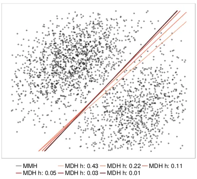
MDH h: 0.05 MDH h: 0.43MDH h: 0.03 MDH h: 0.22MDH h: 0.01 MDH h: 0.11
Figure 3: Convergence of the MDH to the maximum margin hyperplane for a decreasing sequence of bandwidth parameters,h.
Now, since H(vm, bm) is strictly feasible ∃0 >0 s.t. (v, b)∈
B0({(vm, bm),−(vm, bm)})⇒
H(v, b) ∈ FCL. Then for any 0 < < 0 there exists h0 > 0 s.t. for 0 < h < h0 both (vhδ, bδh) ∈B({(vm, bm),−(vm, bm)}) ⇒ H(vhδ, bδh) ∈FCL and H(v?h,η(h),L(h), b?h,η(h),L(h)) ∈
FCLδ . Now forH(v, b)∈FCLδ \FCL we know that ˆI(v, b)< fCL(v, b), whereas forH(v, b)∈
FCL,Iˆ(v, b) =fCL(v, b) and therefore the minimiser offCL(v, b) must lie in the neighbour-hood B({(vm, bm),−(vm, bm)}), and the result follows.
To illustrate the convergence of the MDH to the MMH we use the two-dimensional data set shown in Figure 3. The data is sampled from a mixture of two Gaussian dis-tributions with equal covariance matrix. The MDH with respect to the true underlying density is H((1,−1),0). A large margin separator is artificially introduced by removing a few observations in a narrow margin around a hyperplane different fromH((1,−1),0). The margin is intentionally small to ensure that identifying the MMH is non-trivial. Figure 3 illustrates the MDH solutions arising from the MDP2 method for a decreasing sequence of bandwidths, h. Initially the MDH approximately coincides with the optimal MDH with respect to the true density of the Gaussian mixture. Ash decreases, the MDH approaches the MMH and for the smallest values ofh the two are indistinguishable.
3.2 MDP2 for Semi-Supervised Classification
that for allh∈(0, h0), the optimal hyperplaneH(v?h,η,L,γ, b?h,η,L,γ) correctly classifies all the labelled examples. If this holds, then fSSC(vh,η,L,γ? , b?h,η,L,γ) = fCL(vh,η,L,γ? , b?h,η,L,γ) for all sufficiently smallh, and hence Lemma 6 can be applied to establish the result. The proof relies on the fact that the penalty terms associated with the known labels in Equation (16) are polynomials inb. Provided that γ is bounded below by a polynomial inh, the value of the penalty terms for hyperplanes that do not correctly classify the labelled data dominate the value of the density integral as h approaches zero. Therefore the optimal hyperplane must correctly classify the labelled data for small values ofh.
Lemma 7 DefineFLB ={H(v, b)
yi(v·xi−b)>0,∀i= 1, . . . , `}andFCL={H(v, b) µv− ασv 6 b6 µv+ασv} and assume that FSSC =FLB∩FCL 6=∅ and that ∃H(v, b) ∈FSSC
with non-zero margin. For h >0, let L(h) = (e1/2h2√2π)−1, 0< η(h) 6h and γ(h) >hr for some r >0. Then ∃h0>0 s.t. h∈(0, h0)⇒H(v?h,η(h),L(h),γ(h), b?h,η(h),L(h),γ(h))∈FLB. Proof
Consider H(v, b)6∈FLB. Then,
fSSC(v, b)> 1
n√2πhexp(−ν
2
?/2h2) +γ(h)ν?1+> γ(h)ν?1+,
whereν? >0 minimises n√12πhexp(−ν2/2h2)+γ(h)ν1+. Therefore,ν? is the unique positive
number satisfying,
1
n√2πhexp
− ν
2
?
2h2
−ν?
h2
+ (1 +)γ(h)ν?= 0
⇒ν?1− = (1 +)γ(h)n√2πh3exp
ν?2
2h2
⇒ν? >
(1 +)γ(h)n√2πh3 1/1−
.
We therefore have,
fSSC(v, b) > γ(h)
(1 +)γ(h)n√2πh3
1+
1−
= Kγ(h)1−2h
3(1+)
1−
> Kh
2r+3(1+)
1− ,
whereKis a constant which can be chosen independent of (v, b). Finally, for anyH(v0, b0)∈
FSSC with non-zero margin, ∃h0 >0 s.t.
h∈(0, h0)⇒fSSC(v0, b0) = ˆI(v0, b0)< Kh
2r+3(1+)
1− < fSSC(v, b).
Since K is independent of (v, b), the result follows. The final set of inequalities holds since the hyperplane H(v0, b0) is assumed to have non-zero margin, say Mv0,b0 > 0, and hence
ˆ
I(v0, b0)6 h√1
2πexp{−Mv0,b0/2h
4. Estimation of Minimum Density Hyperplanes
In this section we discuss the computation of MDHs. We first investigate the continuity and differentiability properties required to optimise the projection indicesφCL(v) andφSSC(v). Since the domain of both projection indices, φCL(v) and φSSC(v), is the boundary of the unit-sphere in Rdit is more convenient to express v in terms of spherical coordinates,
vi(θ) =
(
cos(θi)Qij−=11sin(θj), i= 1, . . . , d−1
Qd−1
j=1sin(θj), i=d,
(21)
whereθ∈Θ = [0, π]d−2×[0,2π] is called the projection angle. Using spherical coordinates renders the domain, Θ, convex and compact, and reduces dimensionality by one.
As the following discussion applies to both φCL(v) and φSSC(v) we denote a generic projection index φ: Θ→R, and the associated set of minimisers, as,
φ(θ) = min
b∈Af(v(θ), b), (22)
B(θ) =
b∈Af(v(θ), b) =φ(θ) , (23)
where f(v(θ), b) is continuously differentiable, A ⊂ R is compact and convex, and the correspondenceB(θ) gives the set of global minimisers off(v(θ), b) for eachθ. The definition of Ais not critical in our formulation. Setting,
A⊃
min
v∈Sd−1{µv} −ασpc1 −η,vmax∈Sd−1{µv}+ασpc1 +η
, (24)
where σ2pc
1 is the variance of the projections along the first principal component, ensures
that the set of hyperplanes that satisfy the constraint of Equation (7) will be a subset ofA
for all v.
Berge’s maximum theorem (Berge, 1963; Polak, 1987), establishes the continuity ofφ(θ) and the upper-semicontinuity (u.s.c.) of the correspondenceB(θ). Theorem 3.1 in (Polak, 1987) enables us to establish thatφ(θ) is locally Lipschitz continuous. Using Theorem 4.13 of Bonnans and Shapiro (2000) we can further show thatφ(θ) is directionally differentiable everywhere. The directional derivative atθ in the directionν is given by,
dφ(θ;ν) = min
b∈B(θ)Dθf(v(θ), b)
·ν, (25)
whereDθ denotes the derivative with respect toθ. It is clear from Equation (25) thatφ(θ)
is differentiable if Dθf(v(θ), b) is the same for allb∈B(θ). If B(θ) is a singleton then this
condition is trivially satisfied and φ(θ) is continuously differentiable at θ.
It is possible to construct examples in whichB(θ) is not a singleton. However, with the exception of contrived examples, our experience with real and simulated data sets indicates that when h is set through standard bandwidth selection rules B(θ) is almost always a singleton over the optimisation path.
Proof The result follows immediately from the fact that ifB(θ) ={b}is a singleton, then the derivativeDφ(θ) =Dθf(v(θ), b), which is continuous.
Wolfe (1972) has provided early examples of how standard gradient-based methods can fail to converge to a local optimum when used to minimise nonsmooth functions. In the last decade a new class of nonsmooth optimisation algorithms has been developed based on gradient sampling (Burke et al., 2006). Gradient sampling methods use generalised gradient descent to find local minima. At each iteration points are randomly sampled in a radiusεof the current candidate solution, and the gradient at each point is computed. The convex hull of these gradients serves as an approximation of the ε-Clarke generalised gradient (Burke et al., 2002). The minimum element in the convex hull of these gradients is a descent direction. The gradient sampling algorithm progressively reduces the sampling radius so that the convex hull approximates the Clarke generalised gradient. When the origin is contained in the Clarke generalised gradient there is no direction of descent, and hence the current candidate solution is a local minimum. Gradient sampling achieves almost sure global convergence for functions that are locally Lipschitz continuous and almost everywhere continuously differentiable. It is also well documented that it is an effective optimisation method for functions that are only locally Lipschitz continuous.
4.1 Computational Complexity
In this subsection we analyse the computational complexity of MDP2. At each iteration the algorithm projects the data sample ontov(θ) which involvesO(nd) operations. To compute the projection index, φ(θ), we need to minimise the penalised density integral, f(v(θ), b). This can be achieved by first evaluating f(v(θ), b) on a grid of m points, to bracket the location of the minimiser, and then applying bisection to compute the minimiser(s) within the desired accuracy. The main computational cost of this procedure is due to the first step which involves m evaluations of a kernel density estimator withn kernels. Using the improved fast Gauss transform (Morariu et al., 2008) this can be performed in O(m+
n) operations, instead of O(mn). Bisection requires O(−log2ε) iterations to locate the minimiser with accuracy ε.
If the minimiser of the penalised density integralb?= arg minb∈Af(v(θ), b), is unique the
projection index is continuously differentiable atθ. To obtain the derivative of the projection index it is convenient to define the projection function, P(v) = (x1·v, . . . ,xn·v)>. An
application of the chain rule yields,
dθφ=Dθf(v(θ), b?) =DPf(v(θ), b?)DvP Dθv (26)
where the derivative of the projections of the data sample with respect to v is equal to the data matrix, DvP = (x1, . . . ,xn)>; andDθv is the derivative ofv with respect to the
projection angle, which yields a d×(d−1) matrix. The computation of the derivative therefore requiresO(d(n+d)) operations.
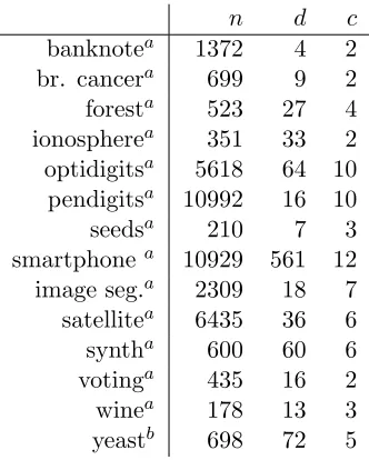
n d c
banknotea 1372 4 2 br. cancera 699 9 2
foresta 523 27 4 ionospherea 351 33 2 optidigitsa 5618 64 10
pendigitsa 10992 16 10 seedsa 210 7 3 smartphonea 10929 561 12 image seg.a 2309 18 7 satellitea 6435 36 6 syntha 600 60 6 votinga 435 16 2 winea 178 13 3 yeastb 698 72 5
a. UCI machine learning repositoryhttps://archive.ics.uci.edu/ml/datasets.html
b. Stanford Yeast Cell Cycle Analysis Projecthttp://genome-www.stanford.edu/cellcycle/
Table 1: Details of benchmark data sets: size (n), dimensionality (d), number of clusters (c).
Lipschitz functions, a simple BFGS method using inexact line searches is much more efficient in practice than gradient sampling, although no convergence guarantees have been estab-lished for this method. BFGS requires a single gradient evaluation at each iteration and a matrix vector operation to update the Hessian matrix approximation. In our experiments we use the BFGS algorithm.
5. Experimental Results
In this section we assess the empirical performance of MDHs for clustering and semi-supervised classification. We compare performance with existing state-of-the-art meth-ods for both problems on the following 14 benchmark data sets: Banknote authentication (banknote), Breast Cancer Wisconsin original (br. cancer), Forest type mapping (forest), Ionosphere, Optical recognition of handwritten digits (optidigits), Pen-based recognition of hand-written digits (pendigits), Seeds, Smartphone-Based Recognition of Human Activities and Postural Transitions (smartphone), Statlog Image Segmentation (image seg.), Statlog Landsat Satellite (satellite), Synthetic control chart time series (synth control), Congres-sional voting records (voting), Wine, and Yeast cell cycle analysis (yeast). Details of these data sets, in terms of their size,n, dimensionality,dand number of clusters,c, can be seen in Table 1.
5.1 Clustering
arbitrary number of clusters. Both take values in [0,1] with larger values indicating a better partition. These measures are motivated by the fact that a good binary partition should (a) avoid dividing clusters between elements of the partition, and (b) be able to discriminate at least one cluster from the rest of the data. To capture this we modify the cluster labels of the data by assigning each cluster to the element of the binary partition which contains the majority of its members. In the case of a tie the cluster is assigned to the smaller of the two partitions. We thus merge the true clusters into two aggregate clusters,C1 and C2.
The first measure we use is the binary V-measure which is simply the V-measure (Rosen-berg and Hirsch(Rosen-berg, 2007) computed onC1, C2 with respect to the binary partition, which we denote Π1,Π2. The V-measure is the harmonic mean of homogeneity and complete-ness. For a data set containing clustersC1, . . . , Cc, partitioned as Π1, . . . ,Πk, homogeneity
is defined as the conditional entropy of the cluster distribution within each partition, Πi.
Completeness is symmetric to homogeneity and measures the conditional entropy of each partition within each cluster,Cj. An important characteristic of the V-measure for
evaluat-ing binary partitions is that if the distribution of clusters within each partition is equal to the overall cluster distribution in the data set then the V-measure is equal to zero (Rosenberg and Hirschberg, 2007). This means that if an algorithm fails to distinguish the majority of any of the clusters from the remainder of the data, the binary V-measure returns zero performance. Other evaluation metrics for clustering, such as purity and the Rand index, can assign a high value to such partitions.
To define the second performance measure we first determine the number of correctly and incorrectly classified samples. The error of a binary partition, E(Π1,Π2), given in Equation (27), is defined as the number of elements of each aggregate cluster which are not in the same partition as the majority of their original clusters. In contrast, the success of a partition, S(Π1,Π2), Equation (28), measures the number of samples which are in the same partition as the majority of their original clusters. The Success Ratio, SR(Π1,Π2), Equation (29), captures the extent to which the majority of at least one cluster is well-distinguished from the rest of the data.
E(Π1,Π2) = min{|Π1∩C1|+|Π2∩C2|,|Π1∩C2|+|Π2∩C1|}, (27) S(Π1,Π2) = min{max{|Π1∩C1|,|Π1∩C2|},max{|Π2∩C1|,|Π2∩C2|}}, (28) SR(Π1,Π2) =
S(Π1,Π2) S(Π1,Π2) + E(Π1,Π2)
. (29)
The Success Ratio takes the value zero if an algorithm fails to distinguish the majority of any cluster from the remainder of the data.
5.1.1 Parameter Settings for MDP2
of local optima, we use multiple initialisations and select the MDH that maximises the
relative depth criterion, defined in Equation (30). The relative depth of an MDH,H(v, b), is defined as the smaller of the relative differences in the density on the MDH and its two adjacent modes in the projected density,
RelativeDepth(v, b) =
minnIˆ(v, ml),Iˆ(v, mr)
o
−Iˆ(v, b)
ˆ
I(v, b) (30)
where ml and mr are the two adjacent modes in the projected density on v. If an MDH
does not separate the modes of the projected density, then its relative depth is set to zero, signalling a failure of MDP2 to identify a meaningful bi-partition. The relative depth is appealing because it captures the fact that a high quality separating hyperplane should have a low density integral, and separate well the modes of the projected density. Note also that the relative depth is equivalent to the inverse of a measure used to define cluster overlap in the context of Gaussian mixtures (Aitnouri et al., 2000). In all the reported experiments we initialise MDP2 to the first and second principal component and select the MDH with the largest relative depth. For the data sets listed above it was never the case that both initialisations led to MDHs with zero relative depth.
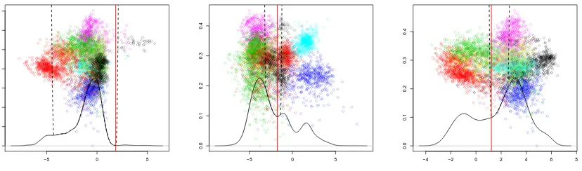
The choice ofα determines the trade-off between a balanced bi-partition and the ability to discover lower density hyperplanes. The difficulties associated with choosing this pa-rameter are illustrated in Figure 4. In each sub-figure the horizontal axis is the candidate projection vector,v, while the right vertical axis is the direction of maximum variability or-thogonal tov. Points correspond to projections of the data sample onto this two-dimensional space, while colour indicates cluster membership. The solid line depicts the projected den-sity on v, while the dotted line depicts the penalised function,fCL(v,·). The scale of both functions is depicted on the left vertical axis. The solid vertical line indicates the MDH alongv. Settingαto a large value can cause MDP2 to focus on hyperplanes that have low density because they partition only a small subset of the data set as shown in Figure 4(a). In contrast smaller values of α may cause the algorithm to disregard valid lower density hyperplane separators (see Figure 4(b)), or for the separating hyperplane to not be a local minimiser of the projected density (see Figure 4(c)).
−5 0 5
0.0
0.1
0.2
0.3
0.4
0.5
0.6
0.7
(a) MDH separating few observa-tions
−5 0 5
0.0
0.1
0.2
0.3
0.4
(b) Lower density hyperplane be-yond feasible region
−4 −2 0 2 4 6 8
0.0
0.1
0.2
0.3
0.4
(c) MDH not a minimiser of the projected density
Figure 4: Impact of choice of α on minimum density hyperplane.
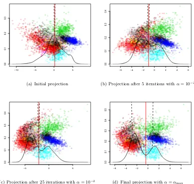
along which the projected density is unimodal and skewed. Figure 5(b) shows that after five iterations withα= 10−2 MDP2has identified a projection vector with bimodal density. In subsequent iterations the two modes become more clearly separated, Figure 5(c), while increasing α enables MDP2 to locate an MDH that corresponds to a minimiser of ˆI(v, b), as illustrated in Figure 5(d).
In all experiments we set the bandwidth parameter toh= 0.9ˆσpc1n−1/5, where ˆσpc1 is the estimated standard deviation of the data projected onto the first principal component. This bandwidth selection rule is recommended when the density being approximated is assumed to be multimodal (Silverman, 1986). The parameter η controls the distance between the minimisers of arg minb∈RfCL(v, b) and arg minb∈F(v)Iˆ(v, b), while larger values ofincrease the smoothness of the penalised functionfCL. Values ofη close to zero affect the numerical stability of the one-dimensional optimisation problem, due to the term ηL infCL becoming very large. We usedη= 10−2 and= 1−10−6 to avoid numerical instability. Beyond these numerical problems the values ofηanddo not affect the solutions obtained through MDP2.
5.1.2 Performance Evaluation
We compare the performance of MDP2 for clustering with the following methods:
1. k-means++ (Arthur and Vassilvitskii, 2007), a version of k-means that is guaranteed to beO(logk)-competitive to the optimal k-means clustering.
2. The adaptive linear discriminant analysis guided k-means (LDA-km) (Ding and Li, 2007). LDA-km attempts to discover the most discriminative linear subspace for clustering by iteratively usingk-means, to assign labels to observations, and LDA to identify the most discriminative subspace.
−10 −5 0 5
0.0
0.1
0.2
0.3
(a) Initial projection
−6 −4 −2 0 2 4 6
0.0
0.1
0.2
0.3
0.4
(b) Projection after 5 iterations withα= 10−2
−5 0 5
0.0
0.1
0.2
0.3
0.4
(c) Projection after 25 iterations withα= 10−2
−6 −4 −2 0 2 4 6
0.0
0.1
0.2
0.3
0.4
0.5
(d) Final projection withα=αmax
Figure 5: Evolution of the minimum density hyperplane through consecutive iterations.
4. The iterative support vector regression algorithm for MMC (Zhang et al., 2009) using the inner product and Gaussian kernel, iSVR-L and iSVR-G respectively. Both are initialised with the output of 2-means++.
5. Normalised cut spectral clustering (SCn) (Ng et al., 2002) using the Gaussian affin-ity function, and the automatic bandwidth selection method of Zelnik-Manor and Perona (2004). This choice of kernel and bandwidth produced substantially better performance than alternative choices considered. For data sets that are too large for the eigen decomposition of the Gram matrix to be feasible we employed the Nystr¨om method (Fowlkes et al., 2004).
space. For the 2-means and LDA-2m algorithm the hyperplane separator bisects the line segment joining the two centroids. iSVR-L directly seeks the maximum margin hyperplane in the original space, while iSVR-G seeks the maximum margin hyperplane in the feature space defined by the Gaussian kernel. PDDP and dePDDP use a hyperplane whose normal vector is the first principal component. PDDP uses a fixed split point while dePDDP uses the hyperplane with minimum density along the fixed projection direction.
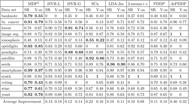
Table 2 reports the performance of the considered methods with respect to the suc-cess ratio (SR) and the binary V-measure (V-m) on the fourteen data sets. In addition Figures 6(a) and 6(b) provide summaries of the overall performance on all data sets using boxplots of the raw performance measures as well as the associated regret. The regret of an algorithm on a given data set is defined as the difference between the best performance attained on this data set and the performance of this algorithm. By comparing against the best performing clustering algorithm regret accommodates for differences in difficulty between clustering problems, while also making use of the magnitude of performance dif-ferences between algorithms. The distribution of performance with respect to both SR and V-m is negatively skewed for most methods, and as a result the median is higher than the mean (indicated with a red dot).
It is clear from Table 2 that no single method is consistently superior to all others, although MDP2 achieves the highest or tied highest performance on seven data sets (more than any other method). More importantly MDP2is among the best performing methods in almost all cases. This fact is better captured by the regret distributions in Figure 6(b). Here we see that the average, median, and maximum regret of MDP2 is substantially lower than any of the competing methods. In addition MDP2 achieves the highest mean and median performance with respect to both SR and V-m, while also having much lower variability in performance when compared with most other methods.
Pairwise comparisons between MDP2 and other methods reveal some less obvious facts. SCn achieves higher performance than MDP2 in more examples (six) than any other com-peting method, however it is much less consistent in its performance, obtaining very poor performance on five of the data sets. The iSVR maximum margin clustering approach is arguably the closest competitor to MDP2. iSVR-L and iSVR-G achieve the second and third highest average performance with respect to V-m and SR respectively. The PDDP al-gorithm is the second best performing method on average with respect to SR, but performs poorly with respect to V-m. The density enhanced variant, dePDDP, performs on average much worse than MDP2. This approach is similarly motivated by obtaining hyperplanes with low density integral, and its low average performance indicates the usefulness of search-ing for high quality projections as opposed to always ussearch-ing the first principal component. Finally, neither of thek-means variants appears to be competitive with MDP2 in general. 5.2 Semi-Supervised Classification
MDP2 iSVR-L iSVR-G SCn LDA-2m 2-means++ PDDP dePDDP
Data set SR V-m SR V-m SR V-m SR V-m SR V-m SR V-m SR V-m SR V-m
banknote 0.79 0.55 0 0 0.35 0 0.46 0.10 0 0.01 0.37 0.01 0.40 0.03 0 0.03
br. cancer 0.91 0.79 0.73 0.56 0.73 0.56 0 0.13 0.87 0.71 0.87 0.72 0.91 0.78 0.90 0.77
forest 0.78 0.67 0.90 0.72 0.91 0.74 0.56 0.41 0.76 0.63 0.72 0.58 0.64 0.36 0 0
image seg. 0.89 0.72 0.82 0.59 0.88 0.71 0.92 0.87 0.78 0.58 0.78 0.71 0.87 0.67 1 1
ionosphere 0.48 0.13 0.47 0.13 0.47 0.13 0.55 0.22 0.47 0.12 0.47 0.12 0.47 0.12 0.42 0.09
optidigits 0.93 0.85 0.63 0.29 0.82 0.60 0 0 0.81 0.62 0.92 0.82 0.68 0.30 0 0
pendigits 0.74 0.39 0.79 0.55 0.88 0.68 0.80 0.68 0.79 0.55 0.78 0.57 0.79 0.54 0.61 0.42
satellite 0.89 0.75 0.73 0.40 0.73 0.40 0.92 0.86 0.73 0.40 0.87 0.81 0.71 0.37 0 0
seeds 0.88 0.73 0.71 0.53 0.71 0.53 0.89 0.76 0.96 0.90 0.86 0.70 0.75 0.59 0.73 0.60
smartphone 0.99 0.97 0.99 0.95 0.99 0.96 0.99 0.94 0.99 0.97 0.99 0.94 0.99 0.95 0 0
synth 0.98 0.94 0.94 0.83 0.94 0.83 1 1 0.88 0.76 1 1 0.69 0.51 1 1
voting 0.70 0.43 0.46 0.09 0 0 0 0.05 0.69 0.41 0 0 0.70 0.40 0.68 0.38
wine 0.77 0.61 0.70 0.52 0.69 0.50 0.67 0.48 0.66 0.48 0.68 0.49 0.65 0.46 0.68 0.49
yeast 0.92 0.76 0.89 0.68 0.91 0.72 0.84 0.61 0.86 0.63 0.91 0.73 0.87 0.65 0 0
Average Improvement 0.13 0.18 0.12 0.14 0.22 0.16 0.10 0.11 0.10 0.08 0.11 0.18 0.40 0.32
Table 2: Performance on the task of binary partitioning. (Ties in best performance were resolved by considering more decimal places)
● ● ● ● ● ● ● ● ● ●
Success Ratio V−measure
0.00 0.25 0.50 0.75 1.00 0.00 0.25 0.50 0.75 1.00 MDP2 iSVR iSVR−G SCn LD A−2m 2−means++ PDDP
dePDDP MDP2 iSVRiSVR−G SCn LD A−2m 2−means++ PDDP dePDDP
(a) Raw Performance Measure
● ● ● ● ● ● ● ● ● ● ● ● ●
Success Ratio V−measure
0.00 0.25 0.50 0.75 1.00 0.00 0.25 0.50 0.75 1.00 MDP2 iSVR iSVR−G SCn LD A−2m 2−means++ PDDP
dePDDP MDP2 iSVRiSVR−G SCn LD A−2m 2−means++ PDDP dePDDP (b) Regret
Figure 6: Performance and Regret Distributions for all Methods Considered
5.2.1 Parameter Settings for MDP2
The existence of a few labelled examples enables an informed initialisation of MDP2. We consider the first and second principal components as well as the weight vector of a linear SVM trained on the labelled examples only, and initialise MDP2 with the vector that minimises the value of the projection index, φSSC. The penalty parameter γ is first set to 0.1 and with this setting α is progressively increased in the same way as for clustering. After this, α is kept at αmax and γ is increased to 1 and then 10. Thus the emphasis is initially on finding a low density hyperplane with respect to the marginal density ˆp(x). As the algorithm progresses the emphasis on correctly classifying the labelled examples increases, so as to obtain a hyperplane with low training error within the region of low density already determined.
5.2.2 Performance Evaluation
To assess the effect on performance of the number of labelled examples, `, we consider a range of values. We compare the methods using the subset of data sets used in the previous section in which the size of the smallest class exceeds 100. In total eight data sets are used. For each value of`, 30 random partitions into labelled and unlabelled data are considered. As classes are balanced in the data sets considered, performance is measured only in terms of classification error on the unlabelled data. For data sets with more than two classes all pairwise combinations of classes are considered and aggregate performance is reported.
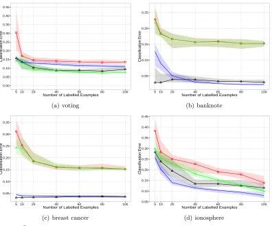
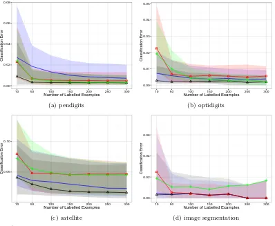
Figure 7 provides plots of the median and interquartile range of the classification error for values of`between 5 and 100 for the four data sets with two classes. Overall MDP2 appears to be most competitive when the number of labelled examples is small. In addition, MDP2 is comparable with the best performing method in almost every case. The only exception is the ionosphere data set where LapSVM outperforms MDP2 for all values of`. Figure 8 provides plots of the median and interquartile range of the aggregate classification error on data sets containing more than two classes. As these data sets are larger we consider up to 300 labelled examples. Note that the interquartile range for XNV is not depicted for the satellite data set. The variability of performance of XNV on this data set was so high that including the interquartile range would obscure all other information in the figure. MDP2 exhibits the best performance overall, and obtains the lowest median classification error, or tied lowest, for all data sets and values of `.
5.3 Summary of Experimental Results
We evaluated the performance of the MDP2 formulation for finding MDHs for both clus-tering and semi-supervised classification, on a large collection of benchmark data sets, and in comparison with state-of-the-art methods for both problems.
● ● ●
●
● ● ●
0.00 0.05 0.10 0.15 0.20 0.25 0.30 0.35 0.40 0.45
5 10 20 40 60 80 100 Number of Labelled Examples
Classification Error
(a) voting
●
●
● ●
● ● ●
0.05 0.10 0.15 0.20 0.25
5 10 20 40 60 80 100 Number of Labelled Examples
Classification Error
(b) banknote
● ● ● ● ● ● ●
0.05 0.10 0.15 0.20 0.25 0.30 0.35
5 10 20 40 60 80 100 Number of Labelled Examples
Classification Error
(c) breast cancer
●
●
● ●
● ●
●
0.05 0.10 0.15 0.20 0.25 0.30 0.35 0.40 0.45
5 10 20 40 60 80 100 Number of Labelled Examples
Classification Error
(d) ionosphere
MDP2 median (—4—), LapSVM median (—◦—), SSSL median (——), XNV
median (—+—), with corresponding interquartile ranges given by shaded regions.
● ●
● ●
● ● ●
0.00 0.02 0.04 0.06 0.08
10 50 100 150 200 250 300 Number of Labelled Examples
Classification Error
(a) pendigits
● ●
● ● ●
● ●
0.00 0.01 0.02 0.03 0.04 0.05
10 50 100 150 200 250 300 Number of Labelled Examples
Classification Error
(b) optidigits
● ●
● ●
●
● ●
0.05 0.10
10 50 100 150 200 250 300 Number of Labelled Examples
Classification Error
(c) satellite
● ● ●
● ●
● ●
0.00 0.02 0.04 0.06
10 50 100 150 200 250 300 Number of Labelled Examples
Classification Error
(d) image segmentation
MDP2 median (—4—), LapSVM median (—◦—), SSSL median (——), XNV median
(—+—), with corresponding interquartile ranges given by shaded regions.
data set, allowed us to summarise the comparative performance of the different methods across data sets. The mean and median raw performance of MDP2 is substantially higher than the next best performing method, and the regret is also substantially lower.
In the case of semi-supervised classification it was apparent that MDP2 is extremely competitive when the number of labelled examples is (very) small, but that in some cases its performance does not improve as much as that of the other methods considered, when the labelled examples become more abundant. Our experiments suggest that overall MDP2 is very competitive with the state-of-the-art for semi-supervised classification problems.
6. Conclusions
We proposed a new hyperplane classifier for clustering and semi-supervised classification. The proposed approach is motivated by determining low density linear separators of the high-density clusters within a data set. This is achieved by minimising the integral of the empirical density along the hyperplane, which is computed through kernel density esti-mation. To the best of our knowledge this is the first direct implementation of the low density separation assumption that underlies high-density clustering and numerous influen-tial semi-supervised classification methods. We show that the minimum density hyperplane is asymptotically connected with maximum margin hyperplane, thereby establishing an important link between the proposed approach, maximum margin clustering, and semi-supervised support vector machines.
The proposed formulation allows us to evaluate the integral of the density on a hyper-plane by projecting the data onto the vector normal to the hyperhyper-plane, and estimating a univariate kernel density estimator. This enables us to apply our method effectively and efficiently on data sets of much higher dimensionality than is generally possible for den-sity based clustering methods. To mitigate the problem of convergence to locally optimal solutions we proposed a projection pursuit formulation.
We evaluated the minimum density hyperplane approach on a large collection of bench-mark data sets. The experimental results obtained indicate that the method is competitive with state-of-the-art methods for clustering and semi-supervised classification. Importantly the performance of the proposed approach displays low variability across a variety of data sets, and is robust to differences in data size, dimensionality, and number of clusters. In the context of semi-supervised classification, the proposed approach shows especially good performance when the number of labelled data is small.
Acknowledgments
(a) (b)
(c) (d)
Proposed MMH —–, Orthogonal hyperplane- - -, Hyperplane with larger margin- · - · -, Regular points , Support points,
Differently assigned support point
Figure 9: Two dimensional illustration of Lemma 9
Memorial Trust. The underlying code and data are openly available from Lancaster Uni-versity data repository at http://dx.doi.org/10.17635/lancaster/researchdata/97.
Appendix A. Proof of Theorem 5
Before proving Theorem 5 we require the following two technical lemmata which establish some algebraic properties of the maximum margin hyperplane. The following lemma shows that any hyperplane orthogonal to the maximum margin hyperplane results in a different partition of the support points of the maximum margin hyperplane. The proof relies on the fact that if this statement does not hold then a hyperplane with larger margin exists which is a contradiction. Figure 9 provides an illustration of why this result holds. (a) Any hyperplane orthogonal to MMH generates a different partition of the support points of MMH, e.g., the point highlighted in red in (b) is grouped with the lower three by the dotted line but with the upper two by the solid line, the MMH. If an orthogonal hyperplane
can generate the same partition (c), then a larger margin hyperplane than the proposed MMH exists (d).
Lemma 9 Suppose there is a unique hyperplane in F with maximum margin, which can be parameterised by (vm, bm) ∈ Sd−1 ×
R. Let M = marginH(vm, bm), C+ = {x ∈
X |vm ·x−bm = M} and C− = {x ∈ X |bm −vm ·x = M}. Then, ∀w ∈ Null(vm),
c∈R eithermin{w·x−c|x∈C+}60, or max{w·x−c|x∈C−}>0.
Suppose the result does not hold, then ∃(w, c) with kwk= 1,w·vm = 0 and min{w·
x−c|x∈C+}>0 and max{w·x−c|x∈C−}<0. Letm= min{|w·x−c|x∈C+∪C−}. Define λ = 2mM < 1. Define u = √ 1
λ2+(1−λ)2(λw+ (1−λ)v
m) and d = λc+(1−λ)bm
√
λ2+(1−λ)2. By
construction kuk= 1. For any x+∈C+ we have, u·x+−d=
λ(w·x+−c) + (1−λ)(vm·x+−bm) p
λ2+ (1−λ)2
> λmp + (1−λ)M
λ2+ (1−λ)2 = m
2+ 2M2−M m p
m2+ (2M−m)2
> M.
Similarly one can show thatd−u·x−> M for anyx−∈C−, meaning that (u, d) achieves
a larger margin onC+ and C− than (vm, bm), a contradiction.
The next lemma uses the above result to provide an upper bound on the distance between pairs of support points projected onto any vector, in terms of the angle between that vector and vm.
Lemma 10 Suppose there is a unique hyperplane in F with maximum margin, which can be parameterised by (vm, bm) ∈ Sd−1×
R. Define M = marginH(vm, bm), C+ = {x ∈
X |vm·x−bm =M}, andC−={x∈ X |bm−vm·x=M}. There is no vector w∈Rd for
which w·x+−w·x−>2Mvm·w for all pairs x+∈C+,x−∈C−.
Proof
Suppose such a vector exists. Define w0 = w−(vm ·w)vm. By construction w0 ∈
Null(vm). For any pairx+∈C+,x− ∈C− we have
w0·x+−w0·x−=w·x+−(vm·w)vm·x+−w·x−+ (vm·w)vm·x− >vm·w(2M−vm·x++bm−bm+vm·x−)
= 0.
Definec:= 12(min{w0·x+
x+∈C+}+ max{w0·x−
x− ∈C−}). Then min{w0·x+−c|x+∈
C+}>0 and max{w0·x−−c|x−∈C−}<0, a contradiction.
We are now in a position to provide the main proof of this appendix. The theorem states that if the maximum margin hyperplane is unique, and can be parameterised by (vm, bm)∈ Sd−1×
R, then
lim
h→0+min{k(v
?
where {H(vh?, b?h)}h is any collection of minimum density hyperplanes indexed by their bandwidth h >0.
Proof of Theorem 5
Define M = marginH(vm, bm), C+ = {x ∈ X |vm ·x−bm = M} and C− = {x ∈ X |bm−vm·x=M}. LetB = max{kxk
x∈ X }. Take any >0 and set 0< δto satisfy 2δ
M(1 +B2) + 2Bδ3/2
q 2
M +δ2=2. Now, suppose (w, c)∈ Sd
−1×
Rsatisfies,
w·x+−c > M−δ, ∀x+∈C+ andc−w·x−> M −δ, ∀x−∈C−.
By Lemma 10 we know that∃x+∈C+,x−∈C− s.t. w·x+−w·x−62Mvm·w. Thus
vm·w> w·x+−w·x−
2M
= w·x+−c+c−w·x− 2M
> 2M−2δ
2M = 1− δ M.
Thus kvm−wk2 < 2δ
M. Now, for each x+ ∈ C
+,vm ·x
+ −b = M and for each x− ∈ C−, b−vm·x−=M. Thus for any suchx+,x− we have,
M−δ+w·x−< c <w·x+−M +δ,
bm−vm·x−−δ+w·x−< c <w·x+−vm·x++bm+δ,
bm−δ−(vm−w)·x− < c < bm+δ+ (w−vm)·x+, bm−δ−Bkvm−wk< c < bm+δ+Bkw−vmk,
|c−bm|<|δ+Bkw−vmk|.
We can now bound the distance between (w, c) and (vm, bm),
k(vm, bm)−(w, c)k2 = kvm−wk2+|bm−c|2
< kvm−wk2(1 +B2) + 2Bδkvm−wk+δ2 < 2δ
M(1 +B
2) + 2Bδ r
2δ M +δ
2 = 2.
We have shown that for any hyperplaneH(w, c) that achieves a margin larger thanM−δ
on the support points of the maximum margin hyperplane, x ∈ C+∪C−, the distance between (w, c) and (vm, bm) is less than. Equivalently, any hyperplaneH(w, c) such that
k(w, c)−(vm, bm)k> has a margin less thanM−δ, as min|w·x−c|
x∈C+∪C− < M−δ. By symmetry, the same holds for any (w, c) within distance of (−vm,−bm).
By Lemma 4 ∃h1 > 0 such that for all h ∈ (0, h1), the minimum density hyperplane for h, H(vh?, b?h), induces the same partition of X as the maximum margin hyperplane,
H(vm, bm). By Lemma 3 ∃h2 >0 such that for allh ∈(0, h2), marginH(vh?, b?h)> M −δ.