Robust Optimal H∞ Control for Uncertain 2-D Discrete Systems described by the General Model via State feedback Controller

(1)

Robust Optimal

H

Control for Uncertain 2-D

Discrete Systems described by the General

Model via State feedback Controller

Arun Kumar Singh

Abstract

This paper is concerned with the problem of H_control for uncertain two-dimensional (2-D) discrete systems described by the General model (GM). The parameter uncertainty is assumed norm-bounded. A sufficient condition to have an Hnoise attenuation for this uncertain 2-D discrete system is given in terms of a certain linear matrix inequality (LMI). A convex optimization problem is proposed to design an optimal



H state feedback controller which ensures stability of the uncertain 2-D discrete system as well as achieving the least value of Hnoise attenuation level of resulting closed-loop system. Finally, an illustrative example is given to demonstrate the applicability of proposed approach.

Keywords Two-dimensional systems; Hcontrol; linear matrix inequality; state feedback controller; general model

I. INTRODUCTION

Along with the growing modern developing technology in industries, the research on Multivariable systems and Multidimensional signals have received considerable attention due to its practical and theoretical interest in the different fields such as thermal processes in chemical reactor, digital filtering, seismographic data processing, water stream heating, data processing, gas absorption, heat exchanger and pipe furnaces, etc have a natural 2-D representation [1, 24, 25, 26]. Therefore, the analysis and synthesis of 2-D discrete systems is an interesting and challenging task, and it has received much attention, for example different 2-D linear state-space models have been proposed by several researchers such as Attasi, Givone-Roesser, Fornasini-Marchesini (FM) [2, 3, 4], Hinamoto (1997) addresses stability of 2-D systems [27], and Bisiacco (1995) presented the 2-D optimal control theory [28]. To effectively solve the noise and/or disturbance attenuation problem for 2-D systems, Sebek (1993) first addressed the H control

problem for 2-D systems [29] and Du and Xie (2002) established several versions of 2-D bounded real lemma [30].

Stability analysis of system is the main issue of designing any control system. When introducing state-space models of 2-D discrete system, many lyapunov equations are used as powerful tools for stability analysis of 2-D discrete system and errors are inevitable as the actual system parameters would be different than the estimated system parameters. These errors changes in the operating conditions, system aging etc. This may lead to instability and degradation in the performance [33]. Therefore, it is desirable to design a control systems which not only stabilize, but also guarantees an adequate level of performance [16]. One approach to this problem is the so called guaranteed cost control approach. This approach has the advantage of providing an upper bound of a given quadratic cost function and thus the system performance degradation incurred by the uncertainties is guaranteed to be less than this bound. Based on this idea, many significant results have been obtained in the literature [11, 13, 14, 15]. Stability analysis and filter design have been addressed in [5, 6, 7, 8, 9, 12].

In recent years, the problem of H control is

an attractive topic in the theory analysis and practical implementation. In various engineering systems time-delay and uncertainty phenomenon appears several times in various engineering systems such as chemical processing, networked control system, aircraft etc. In a dynamic system, instability, oscillations or performance degraded due to the existences of delays and uncertainties. The system stability and performance are two fundamental requirements in the uncertain control system design. A stable system must have a good dynamic performance such as fast response, effective load rejection, and small overshoot. In the past, much attention has been focused on the study of H control

problems where main goal of designing controller is to stabilize the closed-loop system and the Hnorm of

the resulting closed-loop transfer function is minimized.

In the system theory, H norm of the transfer

(2)

reduced. Therefore, time delay and uncertain systems are the most interesting topics in control fields over the decades. A major advantage of Hcontrol is that its

performance specification takes account of the worst-case performance for system in terms of system energy gain [18, 20]. This is suitable for system robustness analysis and robust control with modeling uncertainties and disturbances than other specification. In this paper, we analyze system by H performance measure,

which is an upper bound of maximum gain in the space over all frequencies. The advantage of using the H

performance measure is its lesser sensitivity to uncertainty in the exogenous signal. This has motivated the study of robust H control for uncertain 2-D

discrete systems. To the authors‟ knowledge, the robust



H control for uncertain 2-D discrete systems described by general model (GM) via state feedback controller has not been investigated up to date. GM is one of the best model because it is superset of all state-space models and structurally different from other models.

Therefore, with above motivation, this paper addresses to the problem of H control for uncertain

2-D discrete Systems described by general model. The approach adopted in this paper is as follows: We have developed a sufficient condition for such a system to have specified Hnoise attenuation is first presented

via the LMI approach. To design the optimal H state

feedback controller, LMI constraints are formulated such that for closed-loop system, H noise attenuation

level



is minimized. Finally, the numerical example is given to demonstrate the effectiveness of the proposed method.

Notation

The following notations are used throughout the paper: Rn denotes real vector space of dimension

n

, Rn m denotes the set of nm real matrices, 0 is the null matrix or null vector of appropriate dimension,

I

is the identity matrix of appropriate dimension, the superscript

T

stands for matrix transposition,

{...}

diag stands for a block diagonal matrix, G0

(respectively,G0) denotes a matrix G, which is real symmetric and positive (respectively, negative)

II. PROBLEM FORMULATION AND PRELIMINARIES

This paper deals with the problem of H

control for uncertain 2-D discrete systems described by the GM [3]. Specifically, the system under consideration is given by

1 2 0

( 1 1)

( 1) ( 1 ) ( )

i + , j +

= i, j + + i + , j + i, j x

A x A x A x

1

(

1)

2

(

1 )

0

(

)



B

w

i, j +

+

B

w

i + , j +

B

w

i, j

1 (i, j +1)+ 2 (i + , j +1 ) 0 (i, j)

C u C u C u (1.1a)

(

i j

,

)

=

H

(

i j

,

)

+

L

(

i j

,

)

z

x

w

. (1.1b)

where 0i, jZ (Z denotes a set of integer) are horizontal and vertical coordinates, respectively;

( )

x i, j ∈Rn is the state vector, u(i, j)∈Rm is the input vector, z(i, j)Rp is the controlled output,

( )

w i, j Rq is the noise input which belongs to





2 [0,),[0,)

 and

1 ( 1  1)

A = A + A , A₂=(A₂+A₂),

0 =( 0+ 0)

A A A ,

1 =( 1+ 1)

B B B , B2=(B2+B2), B0=(B0+B0),

1 =( 1+ 1)

C C C , C2 =(C2+C2), C0 =(C0+C0).

(1.1c)

The matrices A1 A A2 0

n n R 

, , , B1 B B2 0

n q

R  

, , ,

1 2 0

C C C n m

R 

, , , HRp n and LRp q are known constant matrices representing the nominal plant. The matrices A1, A2, A0, B1, B2, B0,

1

C

 , C2, and C0 represent parameter uncertainties

in the system matrices, which are assumed to be of the form

1 1 1 0 (i, j +1) 1 4 7

   

   

 A B C H F E E E ,

2 2 2 0 (i + , j1 ) 2 5 8

   

   

 A B C  H F E E E ,

0 0 0 0 (i, j) 3 6 9

   

   

 A B C  H F E E E .

(1.1d)

p n

(3)

1 1

( ,i j ), (i , ), ( , )j i j Rk l

F F F is an unknown

matrix representing parameter uncertainty and satisfies

1 1

( , ) ( , ) , ( , ) ( , ) ,

( , ) ( , ) . T

T T

i j i j

i j i j

i j i j

   

 _ _ _



 _



F F I

(1.2)

For the 2-D system (1.1), assume a finite set of initial conditions, i.e., there exist positive integers

r

1 and

r

2

such that

1

2

0 ,

,

0 ,

( , )

0 ( , )

0 .

i

r

j

r









_

_



x

(1.3)

The following lemmas are essential for our main results.

Lemma 1.1 [21, 22, 23] Let ARn n , 0 ,

  H Rn k 

 E l n

R andQQTRn n be given matrices. Then there exist a positive definite matrix P_{such that}

0 0

[ + ]T [ + ]-  0

A H FE P A H FE Q for allF( , )i j satisfying FT( , ) ( , )i j F i j I, if and

only if there exists a scalar

 

0

such that

1

0 0 1





  _

 

 

P H H A

A E E - Q

T

T T 0. (1.5)

Lemma 1.2 [31, 32]

For real matrices M, L Q, of appropriate dimension,

where M = MT and Q = QT 0 then

T 

0

M + L QL , if and only if

_-1 T















0 M

L

-Q

(1.6)

or equivalently

-1

T















0 -Q

L

.

L

M

(1.7)

Definition 1: The system (1.1) is asymptotically stable

if lim 0

rXr  with w( , )i j 0, u( , )i j 0, and

the initial condition (1.3).

Where X_r sup{ ( , ) :x i j i j r i j, , Z}. Definition 2: Consider system (1.1) with u( , )i j 0 and the initial condition (1.3). Given a

scalar  0, and symmetric positive definite weighting matrices Q Q Q₁, ₂, ₃Rn n , 2-D system (1.1) is said to have an H noise attenuation  if it is

asymptotically stable and satisfies

3

2

2 2

2

1 2

2

sup

0  _{0 )} ₀   J

w

z

= <

w ₊_D _{, j}

₊

_{D i} _{D i j}

.

( ( , ) ( , )

≠ ∈

(1.8)

Where

0 0

2

( 1) ( 1 ) ( )

,

   

 

 

 

 _ _

 

 



z

z z z

i j

i, j +

i + , j

i, j

2

( 1)

= ( 1 )

( )

   

 

 

 

 



w

w w w

i j

i, j + i + , j

i, j

,

1 1

0

0 (0 1) (0 1)







 

( , ) xT , Q x ,

i

D j j j ,

2 2

0

0 ( 1 0) ( 1 0),







 

( , ) xT , Q x ,

j

D i i i and

3 3 3

0 0

(0 ) (0 ) + ( 0) ( 0).

T T

j i

D i j j j i i

 

 





( , ) x , Q x , x , Q x ,

The following theorem presents a sufficient condition for 2-D system (1.1) to ensure the asymptotically stability as well as a specified H noise attenuation. Theorem 1 Given a positive scalar , system (1.1) with u( , )i j 0 and initial condition (1.3) has a H_∞

noise attenuation  if there exist symmetric positive definite matrices P P P, ₁, ₂Rn n satisfying P₁



2Q₁,

2 2 



2,

P Q and 0 P P1P22Q3,such that the

(4)

_______________________________________________________________________________________

1 1

2 2

0 0

1 1

2 2

0 0

                                            _ _{ } _ 

A A

B B

P

T

T T

1

2

1 2

2

.





 



 



 



 



  



 



 



 



 

  

P H H H L

P P P H H H L

L H L L I

T T

- +

- + + +

-0 0 0 0

0 0 0 0

0

0 0 0 0

(1.9)

_______________________________________________________________________________________

Proof Suppose that there exist P10, P20, and

1 2

  0

P P P such that LMI (1.5) holds. We define a Lyapunov function

1 2

( ( , ))

x



( ( , ))

x



( ( , ))

x

V

i j

V

i j

V

i j

3( ( , ))

V x i j . (1.10) Where

1( ( , )) ( , ) 1 ( , )

T

V x i j x i j P xi j

2( ( , )) ( , ) 2 ( , )

T

V xi j x i j P x i j

3( ( , )) ( , )( 1 2) ( , )

T

V x i j x i j P P P x i j . Thus, it is confirm that ( ( , ))V x i j is positive.

The increment V i( 1,j1) along any trajectory of system (1.1) with u( , )i j 0and w( , )i j 0satisfies

(

1,

1)



V i



j



1

( (

1,

1))

2

( (

1,

1))

V

i

j

V

i

j



x



x



3

( (

1,

1))

V

i

j



x



1( ( , 1)) 2( ( 1, )) 3( ( , ))

V xi j V x i j V xi j

1 1

2 2

0 0

( , 1) ( 1, ) ( , )

T

T T T

T T

i j

i j

i j

     

 _{    }

 _{ }

_  _ _{ } _

    

  

     _

x A A

x A P A

x A A

1 2

( , 1) ( 1, ) ( , )

i j

i j

i j 

 

   



   

_  _{ }_  _



      

   

0 0

P x

P P P x

.

It follows from the LMI (1.5) that V i( 1,j 1) 0, i.e.

       

Let us assume that

   

{ , :   : 0, 0}

D r i j i j r i j (1.12)

For integer

r max r r



 

1

,

2

,

it follows from (1.10) and

the initial condition (1.3) that

( (

))

i j D r

V x i j

 



( )

,

2 3

( ( )) ( ( )) ( ( )) i j D r

= V x i, j +V x i, j +V x i, j  



( ) 1

1 1 1

1 1

( ( ,0)) ( ( -1,1)) ( ( 2 2)) ( (1, -1)) ( (0 )

= V x r +V x r +V x r - , +...+V x r +V x ,r

2 2

2 2 2

( ( ,0)) ( ( -1,1))

( ( 2, 2)) ( (1, -1)) ( (0 ) +V x r +V x r

+V x r - + ...+V x r +V x ,r

3 3

3 3 3

( ( ,0)) ( ( -1,1))

( ( 2, 2)) ( (1 1)) ( (0 )) +V x r +V x r

+V x r - + ...+V x ,r - +V x ,r

1

1 1

( ( +1,0))

( ( 1)) ( ( -1, 2)) V x r

+V x r, +V x r + ...+ 

1 1 2

2 2

( (1 )) ( (0 1)) ( ( 1,0)) ( ( 1)) ( ( -1, 2))

V x ,r +V x ,r + +V x r + +V x r, +V x r + ...+

2 2 3

3 3

( (1 )) ( (0 1)) + ( ( 1,0)) ( ( 1)) ( ( 1, 2))

V x ,r +V x ,r + V x r + +V x r, +V x r - + ...+

1

2 3

( (1 )) ( (0 1)) ( ( 1 1)) ( ( 1 1)) - ( ( 1 1)) =

3 3

V x ,r +V x ,r + -V x - ,r + -V x r + ,- V x -

,-1 1

1

( ( )) ( ( 2 )) ( ( 1 1))

( ( 2)) i j D r

V x i j V x r + ,0 +V x r + , +V x r, + ...+

  





( )

,

(5)

3 3 1

2 3

( (1 1)) ( (0 2)) ( ( 1 1)) ( ( 1 1)) - ( ( 1 1))

V x ,r + +V x ,r + -V x - ,r + -V x r + ,- V x - ,-

-1 2

3

2

( ( 2 2)) ( ( 2 2)) - ( ( 2,-2)) ( ( ))

i j D r V x - ,r + -V x r +

,-V x - = V x i, j  





( ) ( )

(1.13)

This implies that the whole energies stored at the points is strictly less than those at the points

 



i, j : i + j = r +1



and the whole energies stored at the points



 

i, j : i + j = r +1



is strictly less than

those at the points



 

i, j : i + j = r



. i.e.

 







 



 





2 1

E E

E

i, j : i + j = r + i, j : i + j = r +

i, j : i + j = r

 

unless all

x i, j =

 

0.

Thus we get

   ,



 



lim , 0

r

i j D r

V x i j





_  (1.14)

It follows that

 





lim x , 0

i j V i j  , i+ jlim→∞x

 

i j, 0. Here, we bring to a close that from above the system (1.1) is asymptotically stable.

Now for the H_∞ performance of system (1.1) with control input u

 

i j, 0for

 

i j,  2





0,



,[0, ) ,



w  we consider





 

1

( 1) ( 1)

1 ( 1 ) ( 1 )

   

   

   



z z

T

i, j + i, j + V i + , j + + i + , j i + , j

i, j i, j









 









 

2

1 1



   

   

   

w w

T

i, j + i, j + - i + , j i + , j

i, j i, j

1 1

2 2

0 0

1 1

2 2

0 0

1 1

T

T T

T

i j i j

i j i j i j

i j

   

   

 

 

 

 



 



 



 

 _

 



 



 



 

   

   

  

 

  ( , ) ( , ) ( , ) ( , ) ( , ) ( , )

A A

P

A A

B B

x x x w w w

1

2

1 2 

        

P H H

P P P H H

L H

T

- +

- + + +

0 0

2

2 



        

H L

H L L L I

L L I

T

-0 0

0 0

( , 1) ( 1, ) ( , ) ( , 1) ( 1, ) ( , ) x x x w w w

i j i j

i j i j i j

i j

 

 

 



 

. (1.15)

It follows from LMI (1.5) that





 

( 1) ( 1)

1 1 ( 1 ) ( 1 )

   

   

 _ _{ } _

   

   

z z

T

i, j + i, j + V i + , j + + i + , j i + , j

i, j i, j









 









 

2

1 1

1, 1, 0



   

   _{ }

   

   

w w

T

i, j + i, j + - i + j i + j

i, j i, j

.

(6)





 

0 0

( 1) ( 1)

1 1 ( 1 ) ( 1, ) T

i j

i, j + i, j + V i + , j + + i + , j i + j

i, j i, j  

 

   

   

 _ _{ } _

   

   

    



zz zz

z z









 









 

2 ₁ ₀

1 1

1 T

i, j + i, j + -γ i + , j i + , j

i, j i, j 

   _{ }

   _{ }

   _{ }



w w

. (1.16)

So, from equation (1.16)

2 ₂ 2

2 2

0 0

( 1 1) 0

 

 

     



, z w

i j

V i j γ (1.17)

2 ₂ 2

2



2

z w

0 0

( 1 1) i j

V i j  

 

 



  , 



1



0

(0, 1) (0, 1)





 





_ xT P x _

j

j + j +



2



0

( 1, 0) ( 1, 0)





 

 



x P x 

i

T

i + i +



1 2



0

( , 0)( ) ( , 0)





 





_ xT P P P x _

i

i i



1 2



0

(0, )( ) (0, )





 





_ xT P P P x _.

j

j j (1.18) (1.18)

Since P12Q1, 2 2 2,

P Q and 2

2 1  3, P P- P Q the inequality (1.18) leads to

2 2

1 2

0

(0, 1) (0, 1)

 

  

 

  

 _ _

 w



x

z

xT Q

j

j j

2 0

( 1, 0) ( 1, 0)





 





_xT  Q x  _

i

i i



3



0

( , 0) ( , 0)





 





_ xT Q x _

i

i i



3



0

(0, ) (0, )







 





_ xT Q x _{ }.

j

j j (1.19)

2 2 1  3,

P P- P Q in theorem 1 are no longer needed it follows from (1.15) that









 









 

2 2

2

0 0 i 0 j 0

1 1

1, 1,

,

   



   

     

 _  _  _ 

   

   



zz



ww

z w

i j

i, j i, j

i j i j

i, j i j

(1.20)

i.e.,

 

2

0 0 0

2

0 2

3 , ,0 0,

i j i j

i j i j

   

   

  



z



z



z

 

2

 

2

2 2

0 0 0

3



,0

  

  







w w

i i j

i, j i

 

2 2

0

0, .











w

j

j (1.21)

By considering the zero initial conditions ( ,0) (0, ) 0,

xi x j  i j, 0,1,. Then, from system (1.1) we have that z( ,0)i Lw( ,0)i and

(0, )j  (0, ).j

z Lw Thus, we get from (1.21) that

 

₂

 

2

0 0 0 0

2

3 3

   

   





z



w

i j i j

i j, i, j

 

2

 

0

0  0









wT I LTL w

i

i, ( ) i,

 

2

 

0

0  0









wT I LTL w

j

j ( ) j

, , .

It may known from (1.5), that 2I L L- T 0. Thus, for all nonzero w( , ),i j we obtain

2



2

z w , (1.22)

where ₂

 

2

0 0

.

z z

i j i, j  

 





and

 

2 2

0 0

,

w w

i j

i, j  

 





It follows from that 2-D Perseval‟s Theorem [25] that above equation (1.22) is equivalent to

 



1 2



1 2

1 2 , 0,2

max

)

( , sup σ j , j

z z _  _{ }_ _ _ e e _

G G

(1.23)

(7)

1

1, 2 1 2 2 1 1 2 0

(z z ) (z z nz z  )

G H I A A A

2 1 1 2 0

( )

z B zB B L. (1.24)

Remark 2.1: In this system, controller K and disturbance are playing zero-sum game, in which the

cost is (z2₂2 w 2₂). Our aim is to minimize 2

such that the controller can win the game (i.e. achieve negative cost) means

2 ₂ 2

2 2

(z  w ) < 0

2 2 2

2 2

sup z .

w 

 

III.

H

CONTROLLER DESIGN

Consider system (1.1) and the following controller



u( , )i j Kx( , )i j (2.1)

The resulting closed-loop system is given by

1 1

( 1, 1)( +C K) (, 1)

xi j A x i j

2 0

2+ ) ( 1, ) ( 0+ ) ( , )

(

 A C K x i j  A CK xi j

1 ( , 1) 2 ( 1, ) 0 ( , )

B wi j B wi j B wi j

( , ) ( , ) ( , ).

zi j Hxi j Lwi j (2.2) (2.2)

Our aim to design a controller (2.1) so that system (2.2) is asymptotically stable, and theH_∞

norm of transfer function (1.24) from the noise input ( , )i j

w to the controlled output z( , )i j for the closed-loop system (2.2) has a specified H_∞ noise attenuation



 and the controller (2.1) is said to be a



-suboptimal H_∞ controller for system (1.1).

Theorem 2 Given scalars γ> 0,> 0 and if there exist a matrices NRm n and symmetric positive definite matrices , 1, 2

n n R 

P P P such that the following LMI is feasible:

' ' ' '

1 1 1

' ' '

1 2 2

' ' '

1 2 0 0

2 ' '

1 2 ' 2 2 ' 0 '

1 1 2 2 0 0 1 2 0 0 0

1 2 3 4 5 6

7 8                     

P P A N C PH

P P A N C

P P P P A N C

I B L

I B I B A P C N A P C N A P C N B B B P H H

H P L I

H P L

E P E P E P E E E NE

NE

0 0 0 0 0

0 0 0 0 0 0

0 0 0 0 0

0 0 0 0 0 0

0

0 0 0 0 0

0 0 0 0 0 0

0 0

0 0 0 0 0 0 0

0 9                              NE

0 0 0 0 0 0

0 0 0 0 0 0 0

0 0 0 0 0 0 0 0

' ' ' 1 7 ' ' ' ' 2 8 ' ' ' ' 3 9 ' 4 ' ' 5 ' ' 6                       _     _   _     _   

PE E N

PH PE E N

E L E L E I I I I I I I I

0 0 0 0 0 0

0 0 0 0 0

0 0 0 0 0 0 0

0 0 0 0 0 0

0 0 0 0 0 0 0 0 0 0 0 0 0 0 0 0 0 0 0 0 0 0 0

0 0 0 0 0 0 0

.



  

0 (2.3)

Then the closed-loop system (2.1) has a specified H_∞ noise attenuation



and

1

( , )  ( , )

ui j NP xi j (2.4)

is



-suboptimal H_∞ state feedback controller for 2-D system (1.1).

Proof By applying theorem 1 and Lemma (1.1, 1.2), a sufficient condition for the closed-loop system (2.2) to have a specified H_∞ noise attenuation



is that exist P10, P20, andP P1 P20 such

that

1

2 2

0 0 1 1

1

1 1

1 2

1 1 1 1 1 7 7

1

2

2 2 2 1

' 1

0 0 3 1

1

1 4 1

1

2 5 1

1

0 6 1

                          _     _ _{ } _   _ _{ }        

A C K

P H H A C K

I H

H I

I

E E

A K C H P E E K E E K

P

A K C H E E

B L E E

T

T T T T T T T T

T T T T T T T T T

T T T

0 0 0

0

0 0 0

0 0 0 0

0

0 0 0 0

0 0 0 0 0 0 0 0 0 0 0 0 1 1

2 2 8 8

1 3 2 1 4 2 1 5 2 1 6 2             

E E K E E K

E E

E E E E

E E

(8)

0 0 1 2 0

1 1 1 1

1 3 1 4 1 5 1 6

1 1 1 1

2 3 2 4 2 5 2 6

1 1 ' ' 1 1 1

1 2 3 3 9 9 3 4 3 5 3 6

1 2 1 1 1

4 3 4 4 4 5 4 6

1 1 2

5 3 5 4

   

    

    

   

   

    

   

 



    

 

A C K B B B

L

H L

E E E E E E E E

P P P E E K E E K E E E E E E

E E I E E E E E E

E E E E I

T T T T

T T

0 0 0

0 0

1 1

5 5 5 6

1 1 1 2 1

6 3 6 4 6 5 6 6

.



    

 

   

              

  _



E E E E

E E E E E E I E E

T T

T T T T

0

(2.5) Pre-multiplying and post-multiplying both sides of the matrix inequality (2.5) by



_P-1_,_P-1_,_P-1_,

diag I I I I I I I, , , , , ,



and applying

schur Compliments and denoting PP1,

1 1 ,

P PP P P2PP P2 ,and NKP, it follows that

the inequality (2.5) is equal to the LMI (2.3).This completes the proof.

Remark 2.2: It should be observed matrix inequality (2.3) is linear for> 0 andNRm n _{, positive definite}

matrices , 1, 2

n n R 

P P P so we can solve it using Matlab LMI toolbox [34]. If solution is feasible then state feedback controller can be obtain as

1

u( , )i j Kx( , )i j NP x ( , ),i j i.e. Robust control is realized via state feedback.

Furthermore, by solving the following optimization problem:

minimize



2 (2.6) subject to (2.3),

we can obtain H_∞ controller which ensures that the

H_∞ noise attenuation



of the resulting closed-loop system is minimized. This controller (2.1) is called as the optimal H_∞ controller for the system (1.1).

IV. AN ILLUSTRATIVE EXAMPLE

Consider the thermal processes in chemical reactors, heat exchangers and pipe furnaces, which can be expressed in the following partial differential equation [1].

0

( ) ( )

( ) + ( ).

 

  

 

, ,

,

T x t T x t

a T x t bu x,t

x t (3.1)

Where T x t( ,) is the temperature at x (space)

0, x_f

 

  and t (time) 



0, 



,u x t( , )is the input function, and a b₀, are real coefficients.

Denote x i jT( , ) =_TT(i1 ),j TT(i j, )_, it is easy to

1

0 1

= ,

0 0

A _ _

  2

0

0 0

= ,

1

A _t _t

a t

x x

 

_ _ 

    

  

 

0

0 0

= ,

0 0

A _ _

  1

0 , 0

C    

  2

0 ,

C

b t

 

  _

  0

0 . 0

       C

(3.2) Let  t 0.1, x 0.4,a01, and b0.4. By

considering, the problem of H_∞ disturbance attenuation, and uncertainty, the thermal process is modeled in the form (1.1) with

1

0 , 0.004

B   _

  2

0 , 0.004

B   _

  0

0 , 0.004

B   _

 



0.01 0.01 ,



H 0

0.001 0.00 , 0

2 0

H   _

  L0.5,

1

0.005 0

,

0 0.005

E   _

  2

0.005 0

,

0 0.005

E   _

 

3

0.001 0

,

0 0.001

E   _

  4

0.001 , 0

E   _

 

5

0.007 , 0

E   _

  6

0.007 , 0

E   _

  7

0.001 , 0

E   _

 

8

0.002 , 0

E   _

  9

0.003 . 0

E   _

  _(3.3)

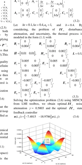
Solving the optimization problem (2.6) using MINCX from LMI toolbox, we obtain optimalH_∞ noise attenuation   0.5003 and the optimal H_∞ state feedback controller



7.4815 18.



( , ) 9786 ( , )

ui j    xi j

(3.4)

Figure 1. The Frequency Response

0 20

40 60

80

0 20 40 60 80 0.4998 0.4999 0.5 0.5001 0.5002 0.5003

w1 (0.1rad/sec) X: 2.539

Y: 3.173 Z: 0.5002

w2 (0.1rad/sec)

IG

(w

1

,w

2

(9)

V. CONCLUSION

This paper has presented a solution to the problem of H∞ Control for 2-D Discrete Uncertain

Systems described by the General Model. A sufficient condition for 2-D discrete uncertain system to have a specified H∞ noise attenuation is proposed in terms

of certain LMI. By solving a convex optimization problem the optimal H∞ controller is obtained. One

example is also given to illustrate the applicability of the proposed approach.

REFERENCES

[1] T. Kaczorek, “Two-dimensional Linear Systems, volume 68 of Lecture Notes in Control and Information Sciences,” Springer-Verlag, Berlin, Germany, 1985.

[2] Fornasini, G. Marchesini, Doubly indexed dynamical systems: State-space models and structural properties, Math. Syst. Theory 12 (1978) 59-72.

[3] Jerzy E. Kurek, “The General State-Space Model for a Two-Dimensional Linear Digital System,” IEEE Transactions on Automatic Control, Vol. AC-30, No. 6, June 1985.

[4] R. P. Roesser, A discrete state-space model for linear image processing. IEEE Transaction Automatic Contol 20 (1975) 1-10.

[5] T. Bose, D. A. Trautman, Two‟s complement quantization in two-dimensional state-space digital Filters. IEEE Transaction Signal Processing 40 (1992) 2589-2592.

[6] T. Bose, Stability of 2-D state-space system with overflow and quantization. IEEE Transaction Circuits System II 42 (1995) 432-434.

[7] T. Zhou, Stability and stability margin for a two-dimensional system. IEEE Trans. Signal Processing. 54 (2006) 3483-3488.

[8] T. Hinamoto, Stability of 2-D discrete systems described by the Fornasini-Marchesini second model. IEEE Trans. Circuits Syst. I 44 (1997) 254-257.

[9] C. Du and L. Xie, Stability analysis and stabilization of uncertain two-dimensional discrete systems: An LMI approach, IEEE Trans. Circuits Syst. I 46 (1999) 1371-1374.

[10] W. Paszke, J. Lam, K. Galkowski, S. Xu, and Z. Lin, Robust stability and stabilization of 2-D discrete state-delayed systems, System Control Letter 51 (2004) 277-291. [11] X. Guan, C. Long, and G. Duan, Robust optimal guaranteed

cost control for 2-D discrete systems, Proc. IEE-Control Theory Appl. 148 (2001) 355-361.

[12] V. Singh, Stability Analysis of 2-D Discrete Systems Described by the Fornasini–Marchesini Second Model with State Saturation, IEEE Trans. Circuits Sysem. II 55 (2008) 793-796.

[13] A. Dhawan and H. Kar, Comment on „Robust optimal guaranteed cost control for 2-D discrete systems‟, IET Control Theory Appication 1 (2007b) 1188–1190.

[14] A. Dhawan and H. Kar, LMI-based criterion for the robust guaranteed cost control of 2-D systems described by the Fornasini–Marchesini second model, Signal Processing 87 (2007a) 479–488.

[15] A. Dhawan and H. Kar, Optimal guaranteed cost control of 2-D discrete uncertain systems: an LMI approach, Signal Processing 87 (2007c) 3075–3085.

[16] L. Xie, C. Du, Y. C. Soh and C. Zhang, Robust control of 2-D systems in FM second model, Multidimensional System Signal Processing 13 (2002) 265-287.

[17] Xu Jian-Ming and Yu Li, “H_∞ Control for 2-D Discrete State Delayed Systems in the Second FM Model,‟‟ Acta Automatica Sinica,Vol.34,No.7,July 2008.

[18] Jianming Xu and Li Yu, “Delay-dependent H_∞ control for 2-D discrete state delay systems in the second FM model,‟‟ Multidimensional Systems and Signal Processing (2009) 20:333–349,

[19] Jianming Xu,Yurong Nan,Guijun Zhang, Linlin Ou, and Hongjie Ni, “Delay-dependent H_∞ Control for Uncertain 2-D Discrete Systems with State Delay in the Roesser Model,‟‟ Circuits System & Signal Process (2013) 32:1097-1112.

[20] Jianming Xu and Li Yu, “H_∞ Control of 2-D Discrete State Delay System,” International journal of control, Automation, and Systems, vol. 4, no. 4, pp. 516-523, August 2006.

[21] X. Guan, C. Long and G. Duan, “Robust optimal guaranteed Cost Control for 2-D Discrete Systems,” IET Control Theory & Applications, Vol. 148, 2001, pp. 355-361.

[22] L. Xie and Y. C. Soh, “Guaranteed Cost-Control of Uncertain Discrete-Time Systems,” Control Theory and Advanced Technology, Vol. 10, 1995, pp. 1235-1251.

[23] A. Dhawan and H. Kar, “Optimal Guaranteed Cost Control of 2-D Discrete Uncertain Systems: An LMI approach,” signal processing, Vol. 87, No.12, 2007, pp. 3075-3085. [24] Bracewell RN (1995) Two-Dimensional Imaging.

Englewood Cliffs, NJ: Prentice-Hall signal Processing Series. [25] Lu W-S and Antoniou A (1992) Two-Dimensional Digital Filters. Electrical Engineering and Electronics, Vol. 80 New York: Marcel Dekker.

[26] Du C, Xu L and Zhang C (2002) H_∞ Control and filtering of Two-Dimensional Systems. Berlin: Springer-Verlag. [27] Hinamoto T. (1997), Stability of 2-D discrete systems

described by the Fornasini-Marchesini second model. IEEE Transactions on circuits systems I: Fundamental Theory and Applications, 44(3), 254-257.

[28] Bisiacco M. (1995) New results in 2-D optimal control theory. Multidimensional systems and signal processing, 6,189-222.

[29] Sebek, M. (1993). H_∞ problem of 2-D systems. European control conference‟93 (pp. 1476-1479).

[30] Du, C., & Xie, L. (2002). H_∞ control and filtering of two-dimensional systems, Lecture Notes in control and information sciences (Vol. 278). Berlin: Springer.

[31] S. Boyd, L. El Ghaoui, E. Feron and V. Balakrishnan, “Linear Matrix Inequalities in System and Control Theory,” SIAM, Philadelphia, 1994.

[32] M. S. Mahmoud, “Robust Control and Filtering for Time- Delay Systems,” Marcel-Dekker, New York, 2000.

[33] Manish Tiwari and Amit Dhawan, “A servey on the stability of 2-D discrete systems described by Fornasini-Marchesini Second model” Circuits and Systems, 2012, 3, 17-22.