Vol. 8, No. 3, 2016 Article ID IJIM-00460, 10 pages Research Article
Estimation of portfolio efficient frontier by different measures of risk
via DEA
M. Sanei ∗, S. Banihashemi†‡, M. Kaveh §
Received Date: 2014-11-27 Revised Date: 2015-05-22 Accepted Date: 2016-03-11
————————————————————————————————–
Abstract
In this paper, linear Data Envelopment Analysis models are used to estimate Markowitz efficient frontier. Conventional DEA models assume non-negative values for inputs and outputs. however, variance is the only variable in these models that takes non-negative values. Therefore, negative data models which the risk of the assets had been used as an input and expected return was the output are utilized . At the beginning variance was considered as a risk measure. However, both theories and practices indicate that variance is not a good measure of risk. Then value at risk is introduced as new risk measure. In this paper,we should prove that with increasing sample size, the frontiers of the linear models with both variance and value at risk , as risk measure, gradually approximate the frontiers of the mean-variance and mean-value at risk models and non-linear model with negative data. Finally, we present a numerical example with variance and value at risk that obtained via historical simulation and variance-covariance method as risk measures to demonstrate the usefulness and effectiveness of our claim.
Keywords: Portfolio; Data Envelopment Analysis (DEA); Value at Risk (VaR); Negative data.
—————————————————————————————————–
1
Introduction
I
npriate mix investments held by an institutionfinancial literature, a portfolio is an appro-or private individuals. Fappro-or investappro-ors, best pappro-ortfo- portfo-lios or assets selection and risks management are always challenging topics. Investors typically try to find portfolios or assets offering less risk and more return. Evaluation of portfolio performance has created a large interest among employees also∗Department of Applied Mathematics, Islamic Azad University of Central Tehran branch, Tehran, Iran.
†Corresponding author. [email protected] ‡Department of Mathematics, Faculty of Mathemat-ics and Computer Science, Allameh Tabataba’i University, Tehran Iran.
§Department of Applied Mathematics, Islamic Azad University of Central Tehran branch, Tehran, Iran.
academic researchers because of huge amount of money are being invested in financial markets. One important idea in portfolio evaluation is the portfolio frontier approach, which measures per-formance of a portfolio by some its distances to the efficient portfolio frontier. In 1952 Markowitz [20] work, laid the base of the frontier approach under the mean-variance (MV) framework. This model was due to the nature of the variance in quadratic form, and tries to decrease variance as a risk parameter in all levels of mean. This model results in an area with a frontier called ef-ficient frontier. Data Envelopment Analysis has proved the efficiency for assessing the relative ef-ficiency of Decision Making Units (DMUs) that employs multiple inputs to produce multiple out-puts (Charnes et al. 1978 [9]). Mean-variance idea has been much extended afterwards, and the
models further being developed along this idea are often referred as nonlinear DEA models.
In 1999 Morey and Morey [23] proposed mean-variance framework based on Data Envelopment Analysis, in which variance of the portfolio is used as an input to DEA models and expected return is used as an output. In 2004 Briec et al. [6] tried to project points in a preferred direction on efficient frontier and evaluate points’ efficien-cies by their distances. Demonstrated model by Briec et al. [7] which is also known as a short-age function, has some advantshort-ages. For example optimization can be done in any direction of a mean-variance space according to the investors’ ideal. Furthermore, in shortage function, effi-ciency of each security is defined as the distance between the asset and its projection in a
pre-assumed direction. As an instance in variance
direction optimization it is equal to the ratio be-tween variance of projection point and variance of asset. Based on this definition if distance equals to zero, that security is on the frontier area and its efficiency equals to 1. This number, in fact, is the result of shortage function which tries to summarize value of efficiency by a number. Simi-lar to any other model, mean-variance model has its own assumptions. Normality is one of its im-portant assumptions. In mean-variance model, distribution of mean of securities in a particu-lar time horizon should be normal. In contrast Mandelbrot [19] showed, not only empirical dis-tributions are widely skewed, but they also have thicker tails than normal. Ariditti [2] and Kraus and Litzenberger [17] also showed that expected return in respect of third moment is positive. Ariditti [2], Kane [15], Ho and Chang [12] showed that most investors prefer positive skewed assets or portfolios, which means that skewness is an output parameter and same as mean or expected return, should be increased. Based on Mitton and Vorkink [22] most investors scarify mean-variance model efficiencies for higher skewed portfolios. In this way Joro and Na [14] introduced mean-variance-skewness framework, in which skewness of returns considered as outputs. Also, Joro and Na reported that the linear DEA estimation of portfolio efficiency is not consistent with the re-sults from their non-linear model. Briec et al. [7] introduced a new shortage function which obtains an efficiency measure which looks to improve both mean and skewness and decreases variance.
Kers-tence et al. [16] introduced a geometric represen-tation of the MVS frontier related to new tools introduced in their paper. In the new models in-stead of estimating the whole efficient frontier, only the projection points of the assets are com-puted. In these models a non-linear DEA-type framework is used where the correlation structure among the units is taken into account. Nowadays, most investors think consideration of skewness and kurtosis in models are critical. Mhiri and Prigent [21] analyzed the portfolio optimization problem by introducing higher moments of return – the main financial index. However, using this approach needs variety of assumptions hold, there is not a general willingness to incorporate higher order moments. Up to this point the assumption is that variance is a parameter that evaluates risk and it is preferred to be decreased, although, not everybody wants this. For example a venture cap-italist prefers risky portfolios or assets, followed by more return than normal. In mean-variance models evaluation,such situations are considered as undesirable situations. But they are not really undesirable for those who are interested in risk for higher returns. There are some approaches, try-ing to address such ambiguities by introductry-ing other parameters, such as semi variance. How-ever, each approach has its own disadvantage which makes it less desirable. A new approach to manage and control risk is value at risk (VaR)
approach. This new approach focuses on the
left hand side of the range of normal distribu-tion where negative returns come with high risk. Value at risk was first proposed by Baumol [4]. The goal is to measure loss of return on left side of the portfolio’s return distribution by report-ing a number. Based on VaR definition, it is as-sumed that securities have a multivariate normal distribution but they also work on non-normal securities. Silvapulle and Granger [28] estimated VaR by using ordered statistics and nonparamet-ric kernel estimation of density function. Chen and Tang [10] investigated another nonparamet-ric estimation of VaR for dependent financial re-turns. Bingham et al. [5] studiedVaR by using semi-parametric estimation of VaR based on nor-mal mean-variance mixtures framework. A fully nonparametric estimation of dynamic VaR is also
developed by Jeong and Kang [13] basedon the
[3] calculated VaR for Greek Stocks by employing nonparametric methods, such as historical and filtered historical simulation. Recently, the non-parametric quantile regression, along with the ex-treme value theory, is applied by Schaumburg [25] to predict VaR. All together Using VaR as a risk controlling parameter is the same as variance; a similar framework is applied: variance is replaced by VaR and then it is decreased in a mean-VaR space. In this study value at risk is decreased in a mean-value at risk framework with negative data. Note that value at risk can be negative, so it is unlikely that variance to get non-negative values.
Conventional DEA models, as used by Morey and Morey [23], assume non-negative values for inputs and outputs. These models cannot be used for the case in which DMUs include both nega-tive and posinega-tive inputs and/or outputs. Portela et al. [24] consider a DEA model which can be ap-plied in cases where input/output data take pos-itive and negative values. There are also other models can be used for negative data such as Modified slacks-based measure model (MSBM), Sharp et. al. [26], semi-oriented radial measure
(SORM), Emrouznejad [11]. In 2015 Lio et al.
[18] demonstrated that the linearized diversifica-tion models can provide an effective way to ap-proximate portfolio efficiency (PE or Markowitz frontier) provided that the frontier is concave. In this paper,we should prove that with increasing sample size, the frontiers of the linear models with both variance and value at risk , as risk measure, gradually approximate the frontiers of the mean-variance and mean-value at risk models and non-linear model with negative data.
The rest of the paper is organized as follows: Section 2 briefly reviews the portfolio perfor-mance literature and have quick look at value at risk as a substitute of variance as a risk pa-rameter. Section 3goes through the convergence property of the RDM models under the mean-variance framework, which indicates that suitable RDM models with sufficient data can be used to effectively approximate the Portfolio Efficiency
(PE). Section 4 presents computational results
using Iranian stock companies data and finally conclusions are given in section5.
2
Background
Portfolio theory to investing is published by Markowitz [20]. This approach starts by assum-ing that an investor has a given sum of money to invest at the present time. This money will be invested for a time as the investor’s holding pe-riod. The end of the holding period, the investor will sell all of the assets that were bought at the beginning of the period and then either consume or reinvest. Since portfolio is a collection of as-sets, it is better that to select an optimal port-folio from a set of possible portport-folios. Hence the investor should recognize the returns (and port-folio returns), expected (mean) return and stan-dard deviation of return. This means that the investor wants to both maximize expected return and minimize uncertainty (risk). Rate of return (or simply the return) of the investor’s wealth from the beginning to the end of the period is calculated as follows:
Return =
(end-of-period wealth)-(beginning-of-period wealth) beginning-of-period wealth
(2.1)
Since Portfolio is a collection of assets, its return
rp can be calculated in a similar manner. Thus according to Markowitz, the investor should view the rate of return associated to any one of these portfolios as what is called in statistics a random
variable. These variables can be described
ex-pected the return (mean orrp) and standard de-viation of return. Expected return and dede-viation standard of return are calculated as follows:
rp = n
∑
j=1
λjrj, σp =
∑n
i=1 n
∑
j=1
λiλjΩij
1 2
(2.2)
Where:
n= The number of assets in the portfolio
rp = The expected return of the portfolio
λj = The proportion of the portfolio’s initial value invested in asset i
rj = The expected return of asset i
iand assetj
minσp =
∑n
i=1 n
∑
j=1
λiλjΩij
1 2 n ∑ j=1
λjrj ≥α
n
∑
j=1
λj = 1
λj ≥0 j= 1, . . . , n
(2.3)
In the above, optimal portfolio from the set of portfolios will be chosen that maximum expected return for varying levels of risk and minimum risk for varying levels of expected return [27]. Data Envelopment Analysis is a nonparametric method for evaluating the efficiency of systems with mul-tiple inputs and mulmul-tiple outputs. In this sec-tion we present some basic definisec-tions, models and concepts that will be used in other sections in DEA. They will not be discussed in details. Consider j, (j = 1, . . . , n) where each consumes
m inputs to produce s outputs. Suppose that
the observed input and output vectors of j are
Xj = (x1j, . . . , xmj) and Yj = (y1j, . . . , ysj) re-spectively, and let Xj ≥ 0 and Xj ̸= 0, Yj and
Yj ̸= 0. A basic DEA formulation in input orien-tation is as follows:
min θ−ε
∑s
r=1
s+r +∑m i=1
s−i
s.t ∑n j=1
λjxij+s−i =θxio i= 1, . . . , m,
n
∑
j=1
λjyrj +s+r =yro r= 1, . . . , s,
(2.4) Whereλis an-vector ofλvariables,s+as-vector of output slacks, s− an m-vector of input slacks and set Λ is defined as follows:
Λ =
{λ∈Rn+ with constant RTS,
{λ∈Rn
+,1λ≤1} with non-increasing RTS,
{λ∈Rn+,1λ= 1} with variable RTS
(2.5)
Note that subscript ’o’ refers to the unit under the evaluation. A is efficient ifθ= 1 and all slack variables s−, s+ equal zero; otherwise it is inef-ficient. In the DEA formulation above, the left –hand sides in the constraints define an efficient portfolio. θ is a multiplier defines the distance from the efficient frontier. The slack variables
are used to ensure that the efficient point is fully efficient. This model is used for asset selection. The portfolio performance evaluation literature is vast. In recent years these models have been used to evaluate the portfolio efficiency. Also in the Markowitz theory, it is required to character-ize the whole efficient frontier but the proposed models by Joro & Na do not need to characterize the whole efficient frontier but only the projec-tion points. The distance between the asset and its projection which means the ratio between the variance of the projection point and the variance of the asset is considered as an efficiency measure (θ). In this framework, there is n assets, λj is the weight of assetjin the projection point,rj is the expected return of asset j,µo and δo2 are the expected return and variance of the asset under evaluation respectively. Efficiency measure θcan be solved via following model:
min θ−ε(s1+s2)
s.t. E ∑n
j=1
λjrj
−s1 =µo,
E ∑n
j=1
λj(rj−µj)
2
+s2 =θδo2
n
∑
j=1
λj ≤1 ∀λ≥0
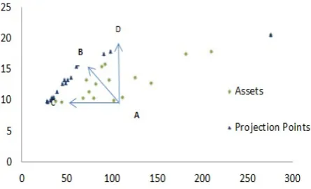
(2.6) Model (2.6) is revealed by the non-parametric efficiency analysis Data Envelopment Analysis (DEA). Fig 1illustrates different projection that
Figure 1: Different projections (input oriented, output oriented, combinationoriented).
via fixing expected return and minimizing
vari-ance, B via maximizing return and minimizing
variance simultaneously, and D via fixing vari-ance and maximizing return.
In the conventional DEA models, each j (j =
1, . . . , n) is specified by a pair of non-negative in-put and outin-put vectors (xj, yj)∈Rm++s, in which
inputs xij (i = 1, . . . , m) are utilized to pro-duce outputs, yrj (r = 1, . . . , s). These models can not be used for the case in which DMUs in-clude both negative and positive inputs and/or outputs. Poltera et al. (2004) [24] consider a DEA model which can be applied in the cases where input/ output data take positive and neg-ative values. Rang Directional Measure (RDM) model proposed by Poltera et al. goes as follows:
max β
s.t. ∑n j=1
λjxij ≤xio−βRio i= 1, . . . , m,
n
∑
j=1
λjyrj ≥yro+βRro r= 1, . . . , s,
n
∑
j=1
λj = 1,
(2.7) Ideal point (I) within the presence of negative data, is I = (maxj{yrj : r = 1, . . . , s},minj{xij :
i= 1, . . . , m}) where
Rio = xio−min
j {xij:j= 1, . . . , n}, i= 1, . . . , m, Rro = max
j {yrj:j = 1, . . . , n} −yro, r= 1, . . . , s.
(2.8)
Here, according to used inputs and outputs, vari-ance (risk parameter) is used as input and mean of returns is used as output in RDM model.
The other models solve negative data such as Modified slacks-based measure model (MSBM), Emrouznejad [11], semi-oriented radial measure (SORM), Sharp et al. [26] and etc. Extremely, we present following non-linear mean-variance RDM
model on the basis of negative data:
max β
s.t. E ∑n
j=1
λjrj
≥µo+βRµo
E
∑n
j=1
λj(rj−µj)
2
≤σo2−βRσ2 o
n
∑
j=1
λj = 1 λ≥0
(2.9) Ideal point (I) within the presence of negative data, isI = (minj{σ2j},maxj{µj}) where
Rµo = max
j {µj : j= 1, . . . , n} −µo
Rσ2
o = σ 2
o−minj {σj2: j= 1, . . . , n}.(2.10)
The above model can be expressed as following:
max β
s.t. E[r(λ)]≥µo+βRµo Var[r(λ)]≤σ2o−βRσ2
o
n
∑
j=1
λj = 1 λ≥0
(2.11)
However, it can be shown that as n increases ,
model (2.7) Converges to models (2.3) & (2.9). Beside variance as a risk parameter which has its positive and negative sides, value at risk (VaR) is another risk parameter with different charac-teristics. To calculate VaR generally there is no need that return’s distributions come from a nor-mal basis, although, the way which is used to obtain VaR, is important.
Value at Risk (VaR) is defined as maximum amount of invest that one may loss in a specified time period. Statistically VaR is defined as the percentile of a distribution.
p(∆Pk>VaR) = 1−α
In historical simulation VaR is calculated based on what happened before. In this method there is no need to be aware of returns distributions over time. Simply returns are order in an ascend-ing way and preferred percentile is value at risk. In fact this method is completely based on what happened before and this is its downside point. When no historical data is available or data have trend, using this method is either impossible or leads to inaccurate results. In contrast with his-torical simulation, variance-covariance method is based on returns distributions. In this method, in the first step, a normality check should be used to get sure, returns come from normal distribu-tion. On the next step, VaR or appropriate per-centile is calculated through formulas obtained based on normal distribution. Value at risk which is calculated from variance covariance method
has its own negative aspects. Wrong
distribu-tion assumpdistribu-tion, non-stadistribu-tionary variables causes by changes happen over time are two of this meth-ods negative points. To calculate VaR from nor-mally distributed returns, consider VaR formulas.
p(∆Pk>−VaR) = 1−α ∆hPt=Pt+h−Pt
(2.12)
By normalizing equation (2.12) we have:
P (
∆hPt−µt
σt
< −VaR−µt σt
)
=α (2.13)
whereZα= ∆hPσtt−µt and Zα ≡Φ−1(α), 12 < α < 1, therefore,
−Zα= −
VaRα−µt
σt
,
and so,
VaRα=σtZα−µt (2.14)
In later sections mean-Var models are introduced and are used to evaluate portfolios efficiencies.
3
Theoretical
foundation
of
RDM
approach:
Conver-gence property
Linear DEA models can’t obtain true solution for estimating portfolio efficient and non-linear RDM frontier. As know, non-linear RDM and Markowitz frontier are concave; therefore we should prove that with increasing sample size,
the frontiers of the RDM linear models gradually approximate the frontiers of the mean-variance model and RDM non-linear model.
Assumption: Suppose there exists a
proba-bility density function p(x) of x ∈ Ω satisfying ∀x0 ∈ Ω, there exists a set S(x0)?U(x0, ξ)∩Ω such that ∫S(x
0)p(x)dx > 0, where U(x
0, ξ) is a
neighborhood of x0x.
Let Ψ = {
(r, σ) | ∑n j=1
λjrj ≥ r, ∑n
j=1
λjσj ≤
σ,∑n
j=1
λj = 1, λj ≥ 0, j = 1, . . . , n
}
, then the
RDM frontier is formed by the outer envelope (upper left boundary) of Ψ as show in Figure 2.
Theorem 3.1 Let rp = h(σp) be the portfolio
frontier without risk-free assets and r∗p+βRr∗p =
h∗n(σp−βRσp) be the RDM frontier with n
port-folio samples. Then h∗n(σp−βRσp) converges to
h(σp) in probability whenn→+∞.
Proof. For any A = (σpa, h(σap)) on the efficient portfolio frontier, there exists xa ∈ Ω, such that (σp(xa), rp(xa)) = (σpa, h(σap)).
Since k(x) ∈(σp(x), rp(x)) is continuous onx, there exists ε > 0, such that k−1(U(A, ε)) is an open set, where U(A, ε) is a neighborhood of A
and
xa∈k−1(U(A, ε)) Thus
∃ξ >0, s.t. S(xa) =U(xa, ξ)∩Ω⊆k−1(U(A, ε)).
Due to the assumption on the probability density functionp(x), we have
q(U(A, ε)) = ∫
k−1(U(A,ε))
p(x)dx >0
≥ ∫
S(xa)
p(x)dx >0
Let T represents the event that the expected re-turns and standard derivations of all the n port-folio samples that are not in U(A, ε). Therefore, the probability of T can be expressed as
P r(T) = (1−q(U(A, ε)))n
It follows from the definition of the concavity of efficient portfolio frontier and RDM frontier that
P r{|h(σap), h∗n(σpa − βRσa
P r{h(σa
p), h∗n(σpa − βRσa
p) > ε} ≤ P r(T) =
(1−q(U(A, ε)))n→0, when n→ ∞.
Because σap is arbitrary, we obtain the conclu-sion that h∗n(σp−βRσp) converges toh= (σp) in
probability, as shown in Figure2.
Figure 2: Convergence explanation. It can be seen as n increases RDM frontier converges to Markowitz frontier.
4
Application in Iranian Stock
Companies
In this section, we verify the validity of the above-discussed results using illustrative examples. 15 stocks from the Iranian stock companies are se-lected, which are monthly data from 21 April 2014 to 21 June 2014. Their statistical properties
are shown in Table ??. We then randomly
gen-eratedn= 10,50,100 weights using MATLAB to construct portfolio samples. Efficiencies of sam-ple portfolios are evaluated with model (2.7). In
Figure 3: Portfolios with different sample sizes.
Figure 3, portfolios with sample sizes 10, 50 and 100 constructed by random weights are shown. In this figure blue curve shows efficient frontier ob-tained by Markowitz model (non-linear model).
By evaluating portfolios’ efficiencies using linear models, it can be seen linear efficient frontier converges to non-linear efficient frontier as n in-creases (Figure 3). In Table 1 statistics of 10
Table 1: Basic statistics of 10 random portfolios made by 15 under evaluation asstes.
Portfolio Mean variance Efficiency
number Mean-var
model (β)
1 -0.0013 0.00012 0.00
2 -0.0001 0.00018 0.18
3 -0.0006 0.00016 0.33
4 -5.5E-05 0.00022 0.30
5 -0.0002 0.00012 0.00
6 -0.0007 0.00017 0.40
7 0.0010 0.00028 0.00
8 6.08E-05 0.00069 0.76
9 -0.0006 0.00017 0.36
10 8E-05 0.00018 0.07
sample portfolios are provided. Statistics for 50 and 100 samples can be calculated in a same way.
As we can see in Table 1 portfolios 1, 5 and 7
are efficient ones. In fact these portfolios are yel-low dots in Figure 3, where the efficient frontier breaks. In Figure 4 efficient RDM frontier for 50
Figure 4: This figure shows as number of samples increases, linear efficient frontier gets closer to non-linear efficient frontier (Portfolio Frontier).
and 100 samples of portfolios are shown. It is obvious by increasing number of samples, linear RDM frontier converges to non-linear frontier.
The three polylines in Figure 4 and 5 are the envelope frontiers constructed by RDM linear models with 10, 50 and 100 samples. The top curve is the efficient frontier calculated by the Markowitz mean-variance model.
eval-Figure 5: Purple dots represent projection of un-der evaluation assets on the efficient frontier.
Figure 6: Mean-VaR region and portfolios. In this plot value at risk is calculated in confidence level of 99%.
uation assets on the efficient frontier which are obtained by solving of non-linear RDM model.
As mentioned in section 2, one may uses value at risk as a risk parameter due to its positive as-pect. In continue, value at risk through two dif-ferent methods for 15 under evaluation assets are calculated. First of all, VaR is calculated by us-ing historical simulation. In this method returns are sorted in an ascending way and appropriate percentile is calculated. Statistics are provided in Table 2. Means are calculated through equation (2.2).
In Table 2, it can be found as the level of value at risk confidence level increases, amount of value at risk gets larger. It illustrates by increasing con-fidence level investor gets more sure how much money may lose in a specified period of invest-ment. Same results for 10 sample portfolios made by 15 assets are provided below. (Table 3)
Figures6-8show portfolios position in a mean-value at risk region. In figures9-11, we can see as the number of samples increases same as
mean-Figure 7: Mean-VaR region and portfolios. In this plot value at risk is calculated in confidence level of 95%.
Figure 8: Mean-VaR region and portfolios. In this plot value at risk is calculated in confidence level of 90%.
Table 2: Mean and value at risk on under evaluation asstes.
Asset Mean Value at Risk
number 90% 95% 99%
1 -0.0007 0.0158 0.0173 0.0217 2 -0.0003 0.0286 0.0370 0.0524 3 -0.0007 0.0347 0.0470 0.0542
4 0.0007 0.0197 0.0269 0.0451
5 0.0001 0.0243 0.0296 0.0439
6 0.0001 0.0373 0.0420 0.0731
7 -0.0053 0.0271 0.0420 0.0729 8 -0.0006 0.0299 0.0405 0.0559 9 -0.0004 0.0191 0.0222 0.0503 10 -0.0011 0.0139 0.0194 0.0298
11 0.0001 0.0210 0.0294 0.0454
12 0.0011 0.0198 0.0273 0.0431
13 -0.0025 0.0233 0.0315 0.0432 14 -0.0003 0.0291 0.0411 0.0545 15 -0.00144 0.0288 0.0321 0.0377
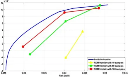
Figure 9: In this figure it can be seen that same as mean-variance models as the number of samples increases linear efficient converges to non-linear frontier. In this figure value at risk is calculated on 99% confidence level.
Figure 10: In this figure it can be seen that same as mean-variance models as the number of samples increases linear efficient converges to non-linear frontier. Value confidence level in this figure is 95%.
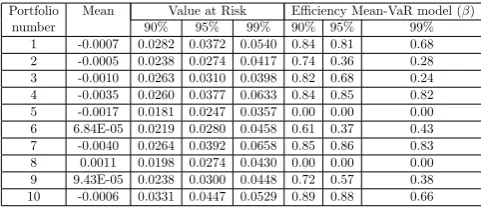
Table 3: Mean and value at risk of 10 portfolios made by under evaluation assets are calculated. Three last columns are their efficiencies and mean-VaR models outputs. Based on this model assets 5 and 8 are effi-cient.
Portfolio Mean Value at Risk Efficiency Mean-VaR model (β) number 90% 95% 99% 90% 95% 99%
1 -0.0007 0.0282 0.0372 0.0540 0.84 0.81 0.68 2 -0.0005 0.0238 0.0274 0.0417 0.74 0.36 0.28 3 -0.0010 0.0263 0.0310 0.0398 0.82 0.68 0.24 4 -0.0035 0.0260 0.0377 0.0633 0.84 0.85 0.82 5 -0.0017 0.0181 0.0247 0.0357 0.00 0.00 0.00 6 6.84E-05 0.0219 0.0280 0.0458 0.61 0.37 0.43 7 -0.0040 0.0264 0.0392 0.0658 0.85 0.86 0.83 8 0.0011 0.0198 0.0274 0.0430 0.00 0.00 0.00 9 9.43E-05 0.0238 0.0300 0.0448 0.72 0.57 0.38 10 -0.0006 0.0331 0.0447 0.0529 0.89 0.88 0.66
In all mentioned figure, value at risk is calcu-lated through historical method, and it was clear that linear frontier is convergence to non-linear frontier. However in some cases frontiers cross
Figure 11: In this figure it can be seen that same as mean-variance models as the number of samples increases linear efficient converges to non-linear frontier. Value confidence level in this figure is 90%.
Figure 12: Sample portfolios in mean-VaR re-gion. Value at risk in calculated based on a 99% confidence level.
each other, mainly they ordered in the way we expect.
Same results are obtained if values at risks are
calculated via variance-covariance method. In
this method, returns have to come from nor-mal distribution. First of all by using Anderson-Darling normality test [1], distributions of returns of under evaluation assets are checked. Returns of 13 assets were normally distributed. For nor-mally distributed assets, expected returns and their value at risks are calculated by using formu-las (2.2). Results are provided in Table 4. Mean and values at risks of normally distributed assets on all level of risk confidence.. Same as histori-cal method, as the risk confidence level increases value at risk of an assets gets larger. Therefore, investor gets surer the amount of risk that may face.
Figure 13: Sample portfolios in mean-VaR re-gion. Value at risk in calculated based on a 95% confidence level.
Figure 14: Sample portfolios in mean-VaR re-gion. Value at risk in calculated based on a 90% confidence level.
Table 4: Mean and values at risks of normally dis-tributed assets on all level of risk confidence.
Asset Mean Value at Risk
number 90% 95% 99%
1 -0.0007 0.0154 0.0197 0.0275 2 -0.0003 0.0309 0.0397 0.0560 3 -0.0007 0.0319 0.0410 0.0576
4 0.0007 0.0234 0.0303 0.0431
5 0.0001 0.0272 0.0351 0.0497
6 0.0001 0.0374 0.0482 0.0682
7 -0.0053 0.0311 0.0386 0.0523 8 -0.0006 0.0350 0.0450 0.0633 9 -0.0004 0.0228 0.0293 0.0412 10 0.0011 0.0212 0.0277 0.0396 11 -0.0025 0.0250 0.0315 0.0434 12 -0.0003 0.0278 0.0358 0.0504 13 -0.0014 0.0254 0.0323 0.0451
linear frontier converges to non-linear one. In Ta-ble5efficiencies of 10 random portfolios made by normal assets are provided.
In Figures15-17, linear efficient frontier of each
Figure 15: Linear and non-linear frontiers with different sample size of portfolios. Linear frontier converges to non-linear frontier and n increases. Value at risk in this figure is calculated in a 99% confidence level.
Figure 16: Linear and non-linear frontiers with different sample size of portfolios. Linear frontier converges to non-linear frontier and n increases. Value at risk in this figure is calculated in a 95% confidence level.
series of sample portfolios are shown.
Table 5: Mean, value at risk and efficiencies of 10 sample portfolios.
Portfolio Mean Value at Risk Efficiency Mean-VaR model (β) number 90% 95% 99% 90% 95% 99%
1 -0.0039 0.0253 0.0314 0.0428 0.90 0.89 0.88 2 -0.0012 0.0225 0.0287 0.0400 0.80 0.78 0.77 3 -0.0006 0.0196 0.0251 0.0352 0.63 0.61 0.59 4 -0.0004 0.0168 0.0216 0.0303 0.00 0.00 0.00 5 -0.0016 0.0187 0.0236 0.0327 0.72 0.70 0.69 6 -0.0002 0.0236 0.0303 0.0428 0.76 0.75 0.73 7 7.6E-05 0.0313 0.0403 0.0570 0.87 0.86 0.85 8 -0.0010 0.0178 0.0226 0.03162 0.57 0.54 0.53 9 0.0003 0.0188 0.0243 0.0345 0.00 0.00 0.00 10 0.0001 0.0363 0.0469 0.0662 0.90 0.90 0.89
Figure 17: Linear and non-linear frontiers with different sample size of portfolios. Linear frontier converges to non-linear frontier and n increases. Value at risk in this figure is calculated in a 90% confidence level.
5
Conclusion
In this paper, under section2, mean-variance, lin-ear and non-linlin-ear RDM models are discussed. In later parts value at risk as a new risk param-eter was discussed. We had also a quick review over methods of VaR calculation and talked about positive and negative aspects of each method. In section3a theorem discussed and proved that by increasing number of samples linear RDM fron-tier convergence to Markowitz fronfron-tier. So RDM linear models can be used to estimate portfolios efficiencies and actual efficient frontier.
In the last section, all discussed topics, with a random sample of stocks data from Tehran stock, was tested. 15 stocks from Tehran stock were ran-domly gathered and their prices over 60 days were gathered. It was shown, as the number of sam-ples increase, whether consider variance or value at risk as a risk parameter, RDM linear frontier converges to Markowitz frontier.
References
[1] T. W. Anderson, D. A. Darling, A Test of
Goodness-of-Fit, Journal of the American Statistical Association 49 (1954) 765-769.
[2] D. AridittiF, Skewness and investors deci-sions: A reply, Journal of Financial and Quantitative Analysis 10 (1975) 173-176.
[3] T. Angelidis, A. Benos, Value-at-Risk for
Greek stocks Multinational Finance Journal 12 (2008) 67-104.
[4] W. J. Baumol,An Expected Gain-Confidence
Limit Criterion for Portfolio Selection, Man-agement Science 10 (1963) 174-182.
[5] NH. Bingham, R. Kiesel, R. Schmidt, A
Semi-Parametric Approach To Risk Man-agement, Quantitative Finance 6 (2003) 426-441.
[6] W. Briec, K. Kerstens, J. B. Lesourd,Single Period Markowitz Portfolio selection, Per-formance Gauging and Duality: A Varia-tion on The Luenberger shortage FuncVaria-tion, Journal of Optimization Theory and Appli-cations 120 (2004) 1-27.
[7] W. Briec, K. Kerstens, O. Jokung,
Mean-Variance-Skewness Portfolio Performance Gauging: A General Shortage Function and Dual Approach, Management Science 53 (2007) 135-149.
[8] A. Charnes, W. W. Cooper, A. Y.
Seiford, Data Envelopment Analysis:
The-ory, Methodology and Applications, Kluwer Academic Publishers, Boston 1994.
[9] A. Charnes, W. W. Cooper, E. Rhodes,
Mea-suring Efficiency of Decision Making Units, European Journal of Operational Research 2 (1978) 429-444.
[10] S. X. Chen, C. Y. Tang, Nonparametric
In-ference of Value at Risk for Dependent Fi-nancial Returns, Journal of financial econo-metrics 12 (2005) 227-55.
[11] A. Emrouznejad, A Semi-Oriented Radial
Measure for Measuring The Efficiency Of Decision Making Units With Negative Data, Using DEA, European journal of Opera-tional Research 200 (2010) 297-304.
[12] Y. K. Ho, Y. L. Cheung, Behavior of Intra-Daily Stock Return on an Asian Emerging Market, Applied Economics 23 (1991) 957-966.
[13] S.O. Jeong, K. H. Kang, Nonparametric
Es-timation of Value-At-Risk, Journal of Ap-plied Statistics 10 (2009) 1225-38.
[15] A. Kane,Skewness Preference and Portfolio Choice, Journal of Financial and Quantita-tive Analysis 17 (1982) 15-25.
[16] K. Kerstens, A. Mounir, I. Woestyne,
Geometric Representation of The Mean-Variance-Skewness Portfolio Frontier Based Upon The Shortage Function, European Journal of Operational Research 10 (2011) 1-33.
[17] A. Kraus, R. H. Litzenberger, Skewness
Preference and the Valuation of Risk Assets, Journal of Finance 31 (1976) 1085-1100.
[18] W. Liu, Z. Zhou, D. Liu, H. Xiao,Estimation of Portfolio Efficiency via DEA, Omega 52 (2015) 107-118.
[19] B. Mandelbrot, The Variation of Certain
Speculative Prices, Journal of Business 36 (1963) 394-419.
[20] H. M. Markowitz, Portfolio Selection, Jour-nal of Finance 7 (1952) 77-91.
[21] M. Mhiri, J. Prigent,International Portfolio Optimization with Higher Moments, Interna-tional Journal of Economics and Finance 5 (2010) 157-169.
[22] T. Mitton, K. Vorknik, Equilibrium under
Diversification and the Preference Of Skew-ness, Review of Financial Studies 20 (2007) 1255-1288.
[23] M. R. Morey, R. C. Morey, Mutual Fund
Performance Appraisals: A Multi-Horizon Perspective With Endogenous Benchmark-ing, Omega 27 (1999) 241-258.
[24] M. C. Portela, E. Thanassoulis, G. Simp-son, A directional distance approach to deal with negative data in DEA: An application to bank branches, Journal of Operational Re-search Society 55 (2004) 1111-1121.
[25] J. Schaumburg, Predicting Extreme Value
at Risk: Nonparametric Quantile Regres-sion with Refinements from Extreme Value Theory, Computational Statistics and Data Analysis 56 (2012) 4081-4096.
[26] J. A. Sharp, W. Meng, W. Liu, A Modified
Slacks-Based Measure Model for Data Envel-opment Analysis with Natural Negative Out-puts and InOut-puts, Journal of the Operational Research Society 57 (2006) 1-6.
[27] W. F. Sharpe, Investment, Third Edition,
Prentice-Hall (1985).
[28] P. Silvapulle, CW. Granger, Large Returns, Conditional Correlation and Portfolio Di-versification: A Value-At-Risk Approach, Quantitative Finance 10 (2001) 542-51.
Masoud Sanei is Associate pro-fessor of Applied Mathematics in operational Research at Islamic Azad University Central Tehran Branches. His research interest are in the areas of Applied Mathemat-ics, Data Envelopment Analysis, Supply Chains, Finance. He has published re-search articles in international journals of Math-ematics. He is referee and editor of mathematical journals.
Shokoofeh Banihashemi is Assis-tant professor of Applied Math-ematics in operational research at Allameh Tabatabaii Univer-sity. Her research interests are in the areas of Applied Mathematics, Data Envelopment Analysis, Sup-ply Chains, Finance. She has published research articles in international journals of Mathemat-ics. She is referee of mathematical and economics journals.