A new hybrid GA-PSO method for solving multi-period inventory routing problem with considering financial decisions

JIEM, 2013 – 6(4): 909-929 – Online ISSN: 2013-0953 – Print ISSN: 2013-8423 http://dx.doi.org/10.3926/jiem.629

A new hybrid GA-PSO method for solving multi-period inventory

routing problem with considering financial decisions

Masoud Rabbani, Milad Baghersad, Ruholla Jafari

College of engineering, University of Tehran (Iran)

[email protected], [email protected] , [email protected] Received: November 2012

Accepted: August 2013

Abstract:

Purpose:

Integration of various logistical components in supply chain, such as transportation,

inventory control and facility location are becoming common practice to avoid

sub-optimization in nowadays’ competitive environment. The integration of transportation and

inventory decisions is known as inventory routing problem (IRP) in the literature. The problem

aims to determine the delivery quantity for each customer and the network routes to be used in

each period, so that the total inventory and transportation costs are to be minimized. On the

contrary of conventional IRP that each retailer can only provide its demand from the supplier,

in this paper, a new multi-period, multi-item IRP model with considering lateral trans-shipment

and financial decisions is proposed as a business model in a distinct organization. The main

concern of this paper is to propose a new decision making approach usable for an organization

to decide economically whether establish a new agent.

Findings:

Numerical results of new proposed algorithm comparing with GAMS are showed that

the proposed algorithm produce good answers and the unique chromosome represented for the

proposed solving methodology is adaptive with the essence of IRP.

Originality/value:

Motivated by real world and analyzing gap in literature, a new MILP model for

multi-period, multi-item IRP with considering lateral trans-shipment and financial decisions is

proposed and then the model is solved with a new hybrid GA-PSO meta-heuristic algorithm.

The chromosome represented for the proposed solving methodology is unique and is another

contribution of this paper which showed to be adaptive with the essence of IRP problem.

Keywords:

inventory routing problem, lateral trans-shipment, genetic algorithm, particle swarm

optimization, hybrid meta-heuristic

1. Introduction

Nowadays in manufacturing business, especially supply chain issues, there is a rising need for efficient behavior because of competition and reduced profit margins. Also production actors and service providers in the transport industry are facing a more challenging situation compared to last decades. In fact, they have to plan the benefit of the whole chain instead of their own company. Since transportation costs are one of the main supply chain costs, vehicle routing problem (VRP) attracted much interest. However inventory and transportation costs are in conflict. The integration of transportation and inventory decisions in literature is represented by IRP. It is to determine the delivery quantity for each customer and a set of feasible vehicle routes for the delivery of the quantities in each period, subject to the vehicle capacity constraints and the customers’ product requirements and inventory capacity constraints, so that a total inventory and transportation cost is minimized.

The main concern of this research is to propose a practical IRP model considering simultaneously lateral trans-shipment and financial decisions in order to help an organization to decide economically whether establish a new agent. Consequently, a novel MILP formulation is proposed to model the problem. To solve the proposed model, for the first time, a new hybrid GA-PSO meta-heuristic algorithm is developed and some randomly generated test problem is provided to demonstrate the usefulness of the proposed hybrid algorithm. A comparison between hybrid algorithm results and GAMS solutions indicates that the average gap is low and the proposed hybrid method gives totally reliable and good answers.

Section 4. Also the specific coding that is used for solving this problem is described in Section 5. Section 6 presents the proposed methodology output and financial analysis, and finally, the discussing and conclusion are provided in Section 7.

2. Literature Review

As pointed by Andersson, Hoff, Christiansen, Hasle and Løkketangen, (2010), approaches for dealing with IRP vary depending on features such as time, demand, topology, vehicle fleet, inventory, and solution method. In an interesting survey, Moin and Salhi (2007) gave a logistical overview of IRPs. They classified the literature according to the number of time periods, single-period, multi-period and infinite horizon models. In another paper, Andersson et al. (2010) described industrial aspects of combined inventory management and routing in maritime and road-based transportation, and gave a classification and comprehensive literature review of this research area. Here we just review the related IRP papers, for further information the reader can refer to the mentioned review papers.

In conventional IRP, each retailer can only provide its demand from supplier but in the model presented in this paper, retailers also can have lateral trans-shipment. In other words, each retailer can provide its demand from other retailers. Paterson, Kiesmuller, Teunter and Glazebrook (2011) presented a review in inventory models with lateral trans-shipments. This review has shown that lateral trans-shipments have been applied in many different types of inventory system in a varied range of industries. Examples of such models in the literature are Fredrik (2010) and Fredrik (2009). Shen, Chu, and Chen (2011) solved a maritime IRP with trans-shipment in crude oil transportation. They proposed that crude oil can be transported from the depot, either directly or via trans-shipment ports at the input and output ports of a pipeline to costumer harbors to satisfy dynamic demands of the customers. Coelho, Cordeau and Laporte (2012) presented an IRP that allows trans-shipments, either from the supplier to customers or between customers. They considered a multi period IRP with a supplier and a set of customer, where both the supplier and customers incur inventory holding costs. Demand of customers is deterministic and inventories are not allowed to be negative. They assume that only a single vehicle is available. They proposed an adaptive large neighborhood search heuristic to solve the problem. This heuristic manipulates vehicle routes while the remaining problem of determining delivery quantities and trans-shipment moves is solved through a network flow algorithm. Their approach can solve four different variants of the problem: the IRP and the IRP with trans-shipment, under maximum level and order-up-to level policies.

There is a massive gap in the literature on IRPs with considering financial decisions. In a related paper, Chen & Lin. (2009) addressed a multi-period supply chain network design problem with considering several aspects of practical relevance such as those related with the financial decisions that must be accounted for by a company managing a supply chain. They considered decisions to be made comprise the location of the facilities, the flow of commodities and the investments to make in alternative activities to those directly related with the supply chain design. They formulated the problem as a multi-stage stochastic mixed-integer linear programming problem, aimed with maximizing the total financial benefit. They also discussed about a methodology for measuring the value of the stochastic solution in the problem.

up to the complexity of proposed IRP model-spells a need for a new solution method. Therefore, a novel hybrid GA-PSO meta-heuristic algorithm is introduced to solve the proposed MILP model.

3. Soft computing techniques

There are a lot of well-known meta-heuristics applied to solve NP-hard problems. Furthermore, the use of these meta-heuristics (e.g., GA, SA, TS, SS and ATO) is growing more and more. Nowadays, researchers have realized that they are not just interested in solving their own-defined problem by simply using a classic meta-heuristic algorithm, but also improving and adapting that algorithm to fulfill their need to find better solution. As matter of fact this is the attractiveness of meta-heuristic algorithms; on the contrary of heuristics, they can be altered to adapt the problem which they are dealing with. It is exceptionally interesting that researchers are not just trying to alter or to justify existing meta-heuristics to have better answers in minimum consumed time. However, recently they have been exploiting more than one heuristic or meta-heuristic algorithm to acquire a more effective solving approach.

This is precisely the reason behind our applying two of the most renowned meta-heuristics, namely Genetic Algorithm (GA), and Particle Swarm Optimization (PSO). The complexity and uniqueness of the proposed problem in this paper made us study different algorithms and put them into perspective with our problem specialties just to find out their amalgamation could work well.

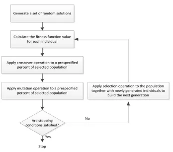
3.1. Genetic Algorithm

Figure 1. Flowchart of genetic algorithm

3.2. Particle swarm optimization Algorithm

PSO is a progressive and also evolutionary calculation algorithm introduced by (Kennedy & Eberhart, 1995). This algorithm has been widely used over these few decades. Though their first algorithm has gone through tangible alteration and modification by other researcher or its innovators themselves, its nature has remained steady and it has been outstandingly in use along the other meta-heuristic algorithms. The algorithm has some similarity with other evolutionary algorithms. It is among population-based search algorithm and also its initialization is completely randomized. Its matchless difference is, however, each individual, called particle, efficiently keeps and uses its own-achieved best answer (pbest) during the competition.

The outline of PSO process is as follows:

1. Initialize a population of particles with uniformly distributed random positions and velocities on d dimensions in the problem space.

2. For each particle, compute the selected optimization fitness function.

3. Compare particle's fitness computation with particle's pbest. If current value is better than pbest, then set the particle’s pbest value and position equal to the current.

5. Change the velocity and Values of the particle according to equations (1) and (2), respectively:

0 ( 1) 1

(

)

2

(

)

idt id t id id d id

v

=

C

×

v

₋

+ × ×

C r

Pb

−

X

+

C

× ×

r

Gb

−

X

(1)

( 1)

idt id t idt

X

=

X

₋

+

v

(2)

Where X: the position of population; i: index for each particle; d: index for each dimension; t: index for each iteration; v: velocity; r: a randomized number with uniform distribution [U(0,1)]; Pb: the position of pbest; Gb: the position of gbest and C0, C1, C2 are Inertia, personal learning and global learning Coefficients, constants to be specified by practitioner.

6. Loop to step (2) until a stop criterion is met, empirically an adequately good fitness or a maximum number of iterations.

The constants which have to be specified by practitioner lead the demeanor and efficacy of the PSO Algorithm. One may deduce the role of constant, C0 called Inertia Coefficient, as a desire of each particle not to change its roaming abruptly. Constants C1 and C2, called respectively personal and Global learning Coefficients, represent weighting of the stochastic motivation terms that draw each particle toward pbest and gbest values respectively. Elaboration of these two constants modifies the amount of tension in the system. Low values allow particles to rove from target area before being tugged back, since high values end in sudden movement toward objective area. Appropriate selection of the inertia coefficient cause a harmony between global and local exploration and exploitation, and results in less iterations to find a sufficient solution (Eberhart & Shi, 2001).

4. Problem definition and MILP model

4.1. Problem description and assumptions

We consider a firm which produces several products and has a set of agents distributed around a particular city. It is been assumed that agents face with different demand for every product (item) in each time period (Dynamic Demand). Agents can store inventory for the next period regarding a holding cost, however, they have limited capacity. In this paper, shortage is permitted with penalty cost and it is treated as lost demand.

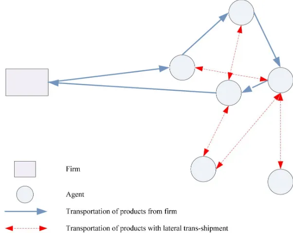
made in the same period. The second types of vehicles are employed between agents when lateral trans-shipment is required. Figure 2 illustrates an example of the proposed model.

Figure 2. An example of the IRP with lateral trans-shipment

As it was mentioned, considered firm produces several items that each of them has different cost of production. Reasonably, selling of each product gains the organization a distinct profit. To formulate the model, due to the complexity of considering production cost, this model is just concerned with the gain due to selling products. This gain is actually the deduction between a product purchase price and production costs (i.e. the costs of raw materials and labor). To clarify, there are two types of costs considered in the model: the costs of inventory and transportation by which our model tries to optimize, and the production costs which are used to calculate the gain of each product.

Apart from the ability of our model to optimize the inventory and transportation costs of an organization in current situation, the model can be used in the decision making process of establishing a new agent. Suppose an organization, already optimized based on this paper’s model, has decided to initiate a development project that is establishing a new agent. The demand of this new agent has been foreseen and it is dynamic, the same as the other agents. This definitely inflicts some charges on organization. These charges may be enumerated by costs related to new building, new staff, adding new production line and so on. However, required fund this new establishment may be acquired by selling bound or distributing new stock.

provide us the information about the exact future income considering the optimized future network. In another words, our model can be used as a mean that provides dependably accurate information about the profitability of establishing new agent. With this valuable information in hand, and considering the costs of establishing a new agent and also the different ways of funding, the organization will be able to decide effectively whether to establish a new agent or not. However, in section 6, a decision procedure with three phases is proposed to help an organization to find whether establishing a new agent has economic justification or not.

4.2. The proposed MILP model

Notations

The following notation is used to formulate the proposed model.

Indices

t

Period index

(

t =

1,...,

T

)

i, j

Agent (retailer) or firm (supplier) index, where

i, j

= 1,...,

N–

1

represent retailer,

N

represent new agent and 0 represents the supplier

s

Product type

(

s =

1,...,

S

)

k

Number of first type’s vehicles

(

k =

1,...

,K

)

Parameters

P

s Revenue (selling price minus purchasing cost and production cost) from the sale a unit

of product

s

Q

1 Each first type’s vehicles capacity

Q

2 Each second type’s vehicles capacity

c

ij Shipping cost along arc

(

i,j

)

where

c

ij

= c

ji and the triangle inequality,

c

il

+ c

lj≤ cij, holds

for any

i, j, l

with

l ≠ i, l ≠ j

p

ij Lateral trans-shipment cost along arc

(

i, j

)

h

i Holding cost per unit of product at retailer

i

and per period

d

ist Demand of product

s

at retailer

i

in period

t

π

is Shortage penalty per unit of product at retailer

i

and per period

i'

Internal rate of return

f

t Inflation rate in period

t

Decision variables

1

0

ijkt

X

= 





If vehicle

k

(first type) travels directly from

i

to

j

in period

t

Otherwise

I

ist Inventory level of product

s

at retailer

i

at the end of period

t

B

ist Shortage quantity of product

s

at period

t

for retailer

i

q

iskt Delivery quantity of product

s

to retailer

i

with vehicle

k

in period

t

1

0

ijt

Y

= 





If we have lateral trans-shipment from

i

to

j

in period

t

Otherwise

T

ijst Delivery quantity of product

s

from retailer

i

to

j

in period

t

with second types of

vehicles (i.e. lateral trans-shipment)

Formulation

1 1 1 1 1 1 1 0, 0 1, 1 1

1

(

)

(

)

(1

)

(1 )

S N S N N S K N N

s ist ist is ist i ist ij ijkt ij ijt t

T

s i s i i s k j j i i

t N j i t N j

Max Z

P d

B

B

h

I

c

X

p Y

f

Subject to: 0 1 1

1,...,

K N jkt k j

X

k

t

T

= =

≤

=

∑∑

(4)

1, 1,

0,..., ,

1,..., ,

1,...,

N N

ijkt jikt

j j i j j i

X

X

i

N k

K t

T

= ≠ = ≠

=

=

=

=

∑

∑

(5)

0 1

1

1,..., ,

1,...,

N jkt j

X

k

K t

T

=

≤

=

=

∑

(6)

1 0,

1

1,..., ,

1,...,

K N

ijkt

k j j i

X

i

N t

T

= = ≠

≤

=

=

∑ ∑

(7)

1 0,

1

1,..., ,

1,...,

K N

ijkt

k i i j

X

j

N t

T

= = ≠

≤

=

=

∑ ∑

(8)

1 1, 1,

1 1

1,..., ,

1,..., ,

1,...,

K N N

iskt jist it ist ijst

k j j i j j

ist ist i

i

st

I

q

T

B

I

T

d

B

j

N

s

S

t

T

= = =

−

≠ ≠ −

+

∑

+

∑

+

=

+

∑

+

+

=

=

=

(9)

1 1 1

1,..., ,

1,...,

S N

iskt

s i

q

Q

t

T k

K

= =

≤

=

=

∑∑

(10)

2 1

,

1,..., ,

,

1,...

,

S ijst s

i j

N j i

T

Q

t

T

=

=

≠

=

≤

∑

(11)

1

1 1 1, 1,

1,..., ,

1,...,

S K N N

ist iskt jist ijst i

s k j j i j j i

I

₋

q

T

T

V

i

N t

T

= = = ≠ = ≠





+

+

−

≤

=

=









∑

∑

∑

∑

(12)

0jt

0

1,..., ,

1,...,

Y

=

j

=

N t

=

T

(13)

0

0

1,..., ,

1,...,

i t

Y

=

i

=

N t

=

T

(14)

(

1)

,

1,..., ,

,

1,...,

1,...,

it jt ijkt

U

−

U

+

N

+

X

≤

N

i j

=

N j i k

≠

=

K t

=

T

(15)

.

,

0,..., ,

,

1,..., ,

1,...,

ijst ijt

T

≤

M Y

i j

=

N j i s

≠

=

S t

=

T

(16)

1 0,

.(

)

1,..., ,

1,..., ,

1,..., ,

1,...,

K N

iskt jikt

k j j i

q

M

X

i

N s

S k

K t

T

= = ≠

≤

∑ ∑

=

=

=

=

(17)

.

1,..., ,

1,..., ,

1,...,

ist ist

I

≤

M F

i

=

N s

=

S t

=

T

(18)

.(1

)

1,..., ,

1,..., ,

1,...,

ist ist

B

≤

M

−

F

i

=

N s

=

S t

=

T

(19)

{ }

0,1

,

1,..., ,

, 1,..., , 1 ,...,

ijkt

0

1,..., ,

1,..., ,

1,...,

ist

I

i

=

N s

=

S t

=

T

(21)

0

1,..., ,

1,..., ,

1,...,

ist

B

i

=

N s

=

S t

=

T

(22)

0

1,..., ,

1,..., ,

1,..., ,

1,...,

iskt

q

i

=

N s

=

S k

=

K t

=

T

(23)

0

,

1,..., ,

,

1,..., , 1 ,...,

ijst

T

i j

=

N i

≠

j s

=

S t

=

T

(24)

1,2, ,

1,..., , 1 ,... ,

it

U

=

…

N

i

=

N t

=

T

(25)

Objective Function (3) calculates difference between revenue and costs of, respectively, shortage, inventory and transportation. Constraint (4) ensures that the number of the first type of vehicles used for delivery in each period does not exceed the total number of first type of vehicles. Constraint (5) ensures that the number of the first type of vehicles leaving from a retailer or the supplier is equal to the number of its arrival. Constraint (6) ensures that each first type of vehicles can travel maximum once in each period. Constraints (7) and (8) ensure that each retailer must be visited maximum once and with one of the first type of vehicles in each period. Constraint (9) is the inventory balance constraints of each retailer at each period. Constraints (10) and (11) ensure that loading of each first and second type of vehicles in each period does not exceed respective capacities. Constraint (12) limits the inventory level of the retailers to the corresponding storage capacity. Constraints (13) and (14) ensure that the second type of vehicles just travel among retailers. Constraint (15) eliminates sub-tours for each first type of vehicles at each period. Constraints (16) and (17) are logical relationships between Yijt, Tijt, Xijkt and qit. Constraints (18) and (19) ensure that at end of each period, each

retailer can’t have both of inventory and shortage. Finally, constraints (20) to (25) show the type of variables.

5. Specific Coding

5.1. General outline

items, and allowing shortage) we decided to apply PSO Algorithm to solve second sub-problem. However, using a meta-heuristic algorithm nested in another one may cause a long time for solving a hybrid approach. To deal with mentioned concern, proposed PSO parameters are set to end in a rather swift solver.

Although there has been a load of efforts and research for the sake of promoting GA operators, the role of defining eligible and qualified chromosome has an impacting influence on the performance of GA. GA chromosome has the most adaptable essence among the other GA concepts, moreover, it can be claimed that it is the superiority point of GA in comparison with the other approaches. Furthermore there had been unprecedented number of unique chromosome in vast gamut of majors and researches. As for this paper, chromosome encoding has given an adaptive characteristic to the algorithm. This fact is actually the reason behind applying the algorithm to the first part of our problem. With this advantage, we managed to inspire the essence of transportation part of the problem to its chromosome. Consequently, this brought about the presentation of crossover and mutation operators.

As for the PSO, Two of the most renowned positive features of PSO are its swiftness and its usability for continuous problems. Latter addresses the continuous feature of inventory problem whereas former satisfies the need for a speedy algorithm. However, to make having another algorithm nested in the other happen we justified the PSO demeanor variables in a way that would end in an as-fast-as-possible algorithm.

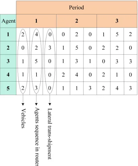
5.2. Chromosome Representation

Figure 3. Chromosome representation

Period Vehicle Sequence of Agents

1 1 Center → 4 → 3 → Center

1 2 Center → 5 → 1 → Center

2 1 Center → 5 → 3 → 2 → Center

2 2 Center → 4 → Center

3 1 Center → 1 → Center

3 2 Center → 4 → 2 → 5 → Center

Table 1. Sequence of each vehicle in each period for chromosome represented in Figure 3

As it is mentioned before, this paper chromosome is unique and has never been in the literature before. However, its greatest improvement is that we have embodied the Lateral trans-shipment concept in the chromosome structure. Furthermore, the chromosome has this advantage over the previous ones that can omit an agent from receiving product from firm in a period. To put it another way, this chromosome has the ability of other renowned VRP chromosome in the literature beside the two mentioned improvements.

5.3. GA Operators

5.3.1. Crossover

Dealing expertly with the GA, one will comprehend the essential role of the crossover operator, which is somehow the means of the GA for the communication between chromosomes. Certainly, it is the agent to converge chromosomes into the optimization. Therefore, the efficacy of the GA is highly depended on a well-operating crossover. The crossover proposed in this paper has proven to be versatile, flexible and adaptive. It uses and merges both undergoing-crossover-chromosome’s (both parent) spirits to make new childes. According to the chromosome in this paper, we introduce multiple crossovers. These distinct crossovers are randomly chosen to be employed in solving procedure.

Regardless of the number agents and machines, we can introduce the proposed chromosome as a single line chromosome with tree different kind of cells (Figure 4) that are Machine Cells (first columns in each period), agent sequence cells (second columns in each period), and lateral trans-shipment cells (third columns in each period). From now on, we know this three kind of cells with respectively first, second, and third cell. The best way to introduce the applied cross over is to say we have simply used the traditional single-break crossover with minor alteration to fulfill the chromosome peculiarity. Imagine the chromosome as a single line with number of period cells, and also think of two child out of mentioned single-break crossover. That is, one of our 7 applied crossovers is just been introduced. The others are just the same with a minor difference. In introduced crossover all of the three cells (columns) were to be transformed between parents. But for other chromosome there is no need for all three cells to be transformed. [1th], [2th], [3th], [1th, 2th], [1th, 3th], [2th, 3th], and [1th, 2th, 3th] are all of the possible ways of engaging each types of cell that makes the mentioned 7 crossovers.

5.3.2. Mutation

Mutation is the agent of the GA not to be stuck in local optimization. Though it does not seem to be an important operator, lack of an eligible mutation probably leads the algorithm to being not effective. Normally, the mutation operator harshly and completely randomly changes the entrance chromosome as long as it remains feasible. Because of abstruseness of the proposed chromosome, there are several ways approaching randomized alteration of chromosome by which we are sure about the chromosome feasibility. We introduce two different mutation operators that make our methodology powerful enough to evade sticking in probable local optimum.

In explanation of applied mutation operator we use the mentioned 1th, 2th, and 3th column in crossover section. This paper methodology uses equally randomly the two distinct mutations. The following is their introductions:

• Choose between mutation 1 or 2 by equal chance

▪ Mutation 1

1. Produced as many as 3*nPeriod*mu randomized numbers. (mu: mutation rate)

2. Cheek for each produced number indicate to which column kind (1th: 0,3,6,9,… 2th:1,4,7,… 3th: 2,5,8,…)

3. For each specified column by produced random number generate a whole new column with respect to the kind of column and the other problem specifications.

▪ Mutation 2

1. Produced as many as 3*nPeriod*nAgent*mu pair of randomized numbers. (mu: mutation rate)

2. Cheek for the first of each pair of produced number indicate to which column kind (1th: 0,3,6,9,… 2th:1,4,7,… 3th: 2,5,8,…)

3. If the first number indicate to 1th column simply produce randomly a new number which is the representative of a machine to replace the indicated number in the chromosome

4. If the first number indicate to 2th column simply produce randomly two number which is the representative of an agent and simply switch the two numbers is indicated by them

5.4. Selection and constant specifying

In order to select chromosome to undergo mutation or crossover we simply omit a proportion of population by pNew rate and randomly by equal chances choose one or two chromosome with respective to the operation, crossover or mutation. Furthermore, because the essence of this paper presented chromosome, crossover or mutation, for every iteration some new chromosome, by the rate of pNew, is initiated. In the process of solving we specified 30, 30, 0.7, 0.1, 0.3, and 0.1 respectively for number of population, number of iterations, crossover percentage, mutation percentage, mutation rate, and new chromosome percentage (pNew).

5.5. Fitness function calculation

As we mentioned earlier, because of the mentioned abstruseness of multi item IRP problem, the process of calculating fitness function in this paper is amalgamated with running PSO process, in another word in every fitness function calculation the PSO process is once run. For the sake of keeping our proposed methodology applicable in matter of time consumption we just took the advantage of PSO initialization process. GA chromosome, as it mentioned in decoding function just specify two of our decision variables, that is

X

ijkt and

Y

ijt respectively

machine kind 1 and lateral trans-shipment routing. Specifying other decision variables, that is,

I

ist

, B

ist

, q

iskt and

T

ijst is the quite massive burden of PSO procedure. Proposed PSO procedure

randomly and with respect to the problem constraints such as Machine and agents capacity specify those unspecified decision variables. Finally, when all of the decision variables are specified fitness value is calculated, using Equation (1) objective.

6. Proposed Methodology Output and Financial Analysis

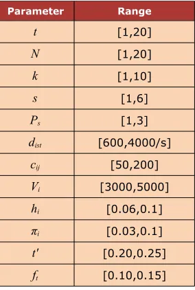
In order to show the applicability and usefulness of the proposed model and solution method, we provide some illustrative examples. To generate the parameters we used uniform distributions. Table 2 shows the range used for generating each parameter. Moreover, we assumed that lateral trans-shipment costs are derived from following equation with α = 0.1. Also, Q1 and Q2 are assumed, respectively, to be 6,000 and 4,000.

(1

)

ij ij

Parameter Range

t [1,20]

N [1,20]

k [1,10]

s [1,6]

Ps [1,3]

dist [600,4000/s]

cij [50,200]

Vi [3000,5000]

hi [0.06,0.1]

πi [0.03,0.1]

t' [0.20,0.25]

ft [0.10,0.15]

Table 2. Range for random generation of parameters

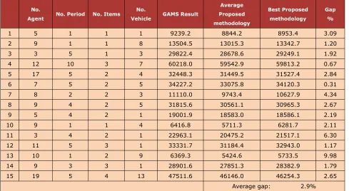
Table 3 shows the influence of problem dimensions on proposed methodology demeanor and Letters ‘S’, ‘M’, and ‘L’ in the second and third column of this table respectively stand for Small, Medium and Large. This table’s aim is to illustrate the influence of Number of Period and Number of Agents on the time of solving. As one can distinguish number of period is a more impacting variable than number of agent on the time of solving. Table 4 shows the comparison between GAMS and proposed methodology results. Note that, due to this paper assumption of existing shortage all of the agents in each period may be given a very different number of products. It can differ from zero to the number of vehicle capacity or the number of agent’s capacity. Therefore, the number of possible solutions even for small problems is infinite and it is logically wrong to consider that the proposed algorithm may result optimum solution. However it is tangibly noticeable that the algorithm finishes in reliable answers.

No. Agent No. Period No. Items No. Vehicle No. Iteration Time consumption

Proposed methodology

1 S 3 S 3 4 4 30 9.7 s 28388.6

2 S 5 M 10 5 4 30 69 s 29494.6

3 S 2 L 17 5 5 30 122.6 s 27355.1

4 M 7 S 5 4 6 30 41.9 s 21461.8

5 M 8 M 9 5 3 30 98.9 s 20793.7

6 M 11 L 20 5 5 30 324.4 s 16234.3

7 L 17 S 6 5 4 30 169.5 s 11714.3

8 L 19 M 8 5 7 30 251.7 s 12842.2

9 L 20 L 19 4 8 30 528.5 s 12799.6

No.

Agent No. Period No. Items

No.

Vehicle GAMS Result

Average Proposed methodology

Best Proposed methodology

Gap %

1 5 1 1 1 9239.2 8844.2 8953.4 3.09

2 9 1 1 8 13504.5 13015.3 13342.7 1.20

3 3 5 1 3 29822.4 28678.6 29249.1 1.92

4 12 10 3 7 60218.0 59542.9 59813.2 0.67

5 17 5 2 4 32448.3 31449.5 31527.4 2.84

6 7 5 2 5 34227.2 33075.8 34120.3 0.31

7 8 2 2 3 11110.0 9743.4 10627.9 4.34

8 9 4 2 5 31815.6 30561.1 30965.3 2.67

9 5 4 2 1 19001.9 18583.0 18586.1 2.19

10 9 1 1 4 6416.8 5711.3 6281.7 2.11

11 3 4 2 1 22963.1 20475.2 21517.1 6.30

12 11 5 3 1 33331.7 31184.4 32943.0 1.17

13 10 1 2 9 6369.3 5424.6 5733.5 9.98

14 9 3 3 1 28901.6 27851.3 28382.9 1.79

15 19 5 4 13 47511.6 46146.0 46254.3 2.65

Average gap: 2.9%

Table 4. Comparison between GAMS and Proposed Methodology

So far in this paper, a new methodology is proposed for those companies who produce several products and have a set of agents in a particular city to decide optimally about the routing and inventory matters in all of their agents. With considering the revenue of each product, inventory, shortage, transportation costs and also inflection and interest rates, the proposed methodology will specifically return the net present income of the company business. As it is mentioned before, the main concern of this paper is to help an organization to decide economically whether establish a new agent. To this end, decision maker(s) should solve the problem in following three phases:

• Solving proposed IRP model and calculating net present income of the company in the

desired horizon without considering new agent in the model.

• Solving proposed IRP model and calculating net present income of the company in the

desired horizon with considering new agent in the model.

• Comparing charges of establishing the new agent and difference between net present

income of the company with considering new agent and without it. If the difference between net present incomes in two cases is greater than charges of establishing the new agent, establishing new company has economic justification.

7. Discussion and Conclusion

lateral trans-shipment and financial decisions in order to help an organization to decide economically whether establish a new agent. Consequently, a MILP model is proposed with the aim of maximizing net present income of the firm regarding purchasing income and its various costs. To solve the proposed model a new hybrid GA-PSO meta-heuristic algorithm is introduced. To demonstrate the usefulness of the proposed hybrid algorithm some randomly generated test problem was provided, the comparison between hybrid algorithm results and GAMS solutions indicated that the average gap is 2.88 percent and the hybrid gives totally reliable and good answers. The most notable upshot can be drawn out of the depicted result is that the proposed hybrid can be applied to real and big problems since GAMS cannot deal with such problems. Finally, a decision procedure with three phases is proposed to help an organization to find whether establishing a new agent has economic justification or not.

Although the hybrid model can produce entitled solutions, it should be noted that a meta-heuristic performance strongly relies on the parameters of it. The setting of parameters is one of the most popular subjects of current research in meta-heuristics. Future research can be base on developing a methodology to tune the proposed hybrid algorithm’s parameters.

References

Abdelmaguid, T.F., Dessouky, M.M., & Ordóñez, F. (2009). Heuristic approaches for the inventory-routing problem with backlogging. Computers & Industrial Engineering, 56(4), 1519-1534.

http://dx.doi.org/10.1016/j.cie.2008.09.032

Andersson, H., Hoff, A., Christiansen, M., Hasle, G., & Løkketangen, A. (2010). Industrial aspects and literature survey: Combined inventory management and routing. Computers & Operations Research, 37(9), 1515-1536. http://dx.doi.org/10.1016/j.cor.2009.11.009

Bard, J.F., & Nananukul, N. (2010). A branch-and-price algorithm for an integrated production and inventory routing problem. Computers & Operations Research, 37(12), 2202-2217.

http://dx.doi.org/10.1016/j.cor.2010.03.010

Bertazzi, L., Bosco, A., Guerriero, F., & Laganà, D. (2011). A stochastic inventory routing problem with stock-out. Transportation Research Part C: Emerging Technologies.

Campbell, A.M., & Savelsbergh, M.W.P. (2004). A Decomposition Approach for the Inventory-Routing Problem. Transportation Science, 38, 488-502. http://dx.doi.org/10.1287/trsc.1030.0054

Chen, Y.M., & Lin, C.-T. (2009). A coordinated approach to hedge the risks in stochastic inventory-routing problem. Computers & Industrial Engineering, 56(3), 1095-1112.

http://dx.doi.org/10.1016/j.cie.2008.09.044

Coelho, L.C., Cordeau, J.-F., & Laporte, G. (2012). The inventory-routing problem with transshipment. Computers & Operations Research, 39(11), 2537-2548.

Eberhart, R.C., & Shi, Y. (2001). Particle swarm optimization: Developments, applications and resources.

Fredrik, O. (2009). Optimal policies for inventory systems with lateral transshipments.

International Journal of Production Economics, 118(1), 175-184.

http://dx.doi.org/10.1016/j.ijpe.2008.08.021

Fredrik, O. (2010). An inventory model with unidirectional lateral transshipments. European Journal of Operational Research, 200(3), 725-732. http://dx.doi.org/10.1016/j.ejor.2009.01.024

Kennedy, J., & Eberhart, R. (1995). Particle swarm optimization.

Lenstra, J.K., & Kan, A.H.G.R. (1981). Complexity of vehicle routing and scheduling problems.

Networks, 11(2), 221-227. http://dx.doi.org/10.1002/net.3230110211

Liu, S.-C., & Chen, J.-R. (2011). A heuristic method for the inventory routing and pricing problem in a supply chain. Expert Systems with Applications, 38(3), 1447-1456.

http://dx.doi.org/10.1016/j.eswa.2010.07.051

Moin, N.H., & Salhi, S. (2007). Inventory Routing Problems: A Logistical Overview. The Journal

of the Operational Research Society, 58(9), 1185-1194.

http://dx.doi.org/10.1057/palgrave.jors.2602264

Paterson, C., Kiesmuller, G., Teunter, R., & Glazebrook, K. (2011). Inventory models with lateral transshipments: A review. European Journal of Operational Research, 210(2), 125-136. http://dx.doi.org/10.1016/j.ejor.2010.05.048

Prins, C. (2004). A simple and effective evolutionary algorithm for the vehicle routing problem.

Computers & Operations Research, 31(12), 1985-2002. http://dx.doi.org/10.1016/S0305-0548(03)00158-8

Shen, Q., Chu, F., & Chen, H. (2011). A Lagrangian relaxation approach for a multi-mode inventory routing problem with transshipment in crude oil transportation. Computers & Chemical Engineering, 35(10), 2113-2123. http://dx.doi.org/10.1016/j.compchemeng.2011.01.005

Journal of Industrial Engineering and Management, 2013 (www.jiem.org)

Article's contents are provided on a Attribution-Non Commercial 3.0 Creative commons license. Readers are allowed to copy, distribute and communicate article's contents, provided the author's and Journal of Industrial Engineering and Management's names are included.