Edge Detection with Hessian Matrix Property Based on Wavelet Transform

Edge Detection with Hessian Matrix Property Based on

Wavelet Transform

N. Aghazadeh and Y. Gholizade Atani

Department of Applied Mathematics, Azarbaijan Shahid Madani University Tabriz 53751 71379, Islamic Republic of Iran

Received: 3 January 2015 / Revised: 30 May 2015 / Accepted: 14 July 2015

Abstract

In this paper, we present an edge detection method based on wavelet transform and

Hessian matrix of image at each pixel. Many methods which based on wavelet

transform, use wavelet transform to approximate the gradient of image and detect edges

by searching the modulus maximum of gradient vectors. In our scheme, we use wavelet

transform to approximate Hessian matrix of image at each pixel, too. The main idea of

our methods lies in the fact that, the direction of largest surface curvature is the

eigenvector of the Hessian matrix corresponding to the largest absolute eigenvalue.

Infact, we use the Hessian matrix's information to increase or decrease the effect of

wavelet transform in and directions.

Keywords: Wavelet transform; Edge detection; Hessian matrix; B-spline Wavelets.

*_{Corresponding author: Tel: +989113966527; Fax:+984134327517; Email: [email protected]}

Introduction

The images are two-dimensional arrays of intensity values with locally varying statistics. However, images have different features which are separated by edges. The edges which have different structures are often the most important assignments in image segmentation [2]. Moreover, edge detection plays an essential role in computer and machine vision [7,18,16], image analysis, pattern recognation, [1], and material processing in the medical imaging, [5,15]. The process of edge detection is based on the hypothesis that the edge is a point where an image has sharp intensity transition [4,14].

Many edge detectors such as Sobel, Roberts, Prewitt, Robinson, Kirsch, Frei-Chen and Marr-Hildreth use the local gradient of the image, [14]. They detect edges by convolving image with a weighted matrix which is called local gradient mask. However, the large class of

edge detectors look up points where the gradient of the image has local maximum. Canny's edge detector is a multiscale version of this approach, [3]. Wheihong Guo and Ming-Jun Lai in [6] peresent a new wavelet frame to detecte edges. In [8], auther proposes an edge detector based on the Green function.

In recent decades, wavelet analysis fostered as a useful research method. The proposed method is based on multiscale wavelet which is one of the new edge detection methods [11]. The traditional edge detectors based on wavelet transform implement the wavelet multiresolution for image firstly, and then pull out the low-frequency sub-image for further process. In the low-frequency sub-image some details and noise will be removed. So, some noise which may be considered as edges are cancelled [3].

by wavelet transform. The paper is organized as follows. Section 2, contains a brief summary of wavelet transform. In section 3, a brief exposition of edge detection and our method is stated. In section 4, we provided several examples for our proposed method and a traditional method.

Materials and Methods

The wavelet transform is a decomposition of signal as a combination of a set of basis functions. These functions are obtained by means of dilation and translation of a original wavelet function ( ). In other word, the continuous wavelet transform of a signal

( )is defined as

( ) =_√ ∫ ( ). , > 0 (1)

However, when the dilation factor grows up, the basis function becomes broader. In this way, the corresponding coefficients give informations about lower frequency components of the signal and vice versa. So, the time resolution at high frequencies is higher than at low frequencies.

If the original wavelet ( ) is derivative of a smoothing function ( ), it can be shown [11,12] that the wavelet transform of a signal ( )at scale is

( ) = − ∫ ( ) ( − ) , (2)

where ( ) =_√ ( ) is the scaled version of the smoothing function. The wavelet transform at scale is correspondence to the derivative of the smoothed signal (which is convolved with ). Therefore, the zero-crossings of the wavelet transform correspond to the local maxima or minima of the smoothed signal at

different scales, and the maximum absolute values of the wavelet transform are associated with maximum stops in the filtered signal.

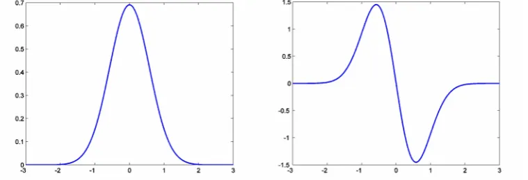
The function ( )is called a smoothing function if its integral is equal to 1 and it tends to zero at infinity. For example, a Gaussian function can be a smoothing function. If one defines ( )as the first derivative of

( ):

( ) = ( ). (3)

then the function ( )can be considered as wavelet, because

∫ ( ) = 0. (4)

Figure 1, shows the smoothing function ( )and its first derivative ( ).

One kind of wavelet systems is biorthogonal wavelet system. Biorthogonal wavelet system has important role in signal and image processing. B-spline wavelet family is one kind of this system. B-spline scaling function are produced by convolving Haar function with itself, [9]. If we write Haar functionϕ( )as

ϕ( ) = ( ) = 1 0 ≤ < 1,_{0 ℎ ,}

(5) then

( ) = ∗ ( ) = 2 − 0 ≤ < 1,1 ≤ < 2,

0 ℎ . (6)

In general case, the B-spline of order n defined by following convolotion,

B-spline wavelets have a fantastic property which allows us to use them in our method. According to [19], we can say the Gaussian function may be an

approximation of B-spline function and their wavelet. The following theorem uses the well-knwon convolution property of B-spline to show that these functions converge to Gaussian as the order of the spline tends to infinity.

Theorem 2.1 [9]. The B-spline function ( ) and its fourier transform ( )both converge to Gaussian as tends to infinity:

lim_→ . ( ) =_√ exp(− ), (8)

lim

→ ( ) = exp − .

(9) Moreover

( )/ converge to exp(− )in

(−∞, +∞) for ∈ [1, +∞), and

converge to exp(− )_√ in (−∞, +∞) for ∈ [2, +∞)as goes to infinity.

Proof.See [19].

For example, the B-spline basis functions of order

= 1 (piecwise linear), and = 3 (cubic spline) are shown in Figure 2. The dotted lines are the Gaussian approximations derived from the previous theorem. As we can see from the proposed figure, the quality of the approximation is pretty good for = 1and = 3.

Now one can approximate the wavelet transform of a signal by convolving the signal with B-spline wavelet, i.e. the wavelet transform of ( ) at the scale and position , wghich computed with respect to the wavelet

( ), may be defined by

( ) ≈ ∗ ( ), (10)

where can be considered as a scaled version of B-spline wavelet. Moreover, theorem 2.1 shows the convolotion between signal ( ) and B-spline scaling function, ( ), produces the smoothed signal.

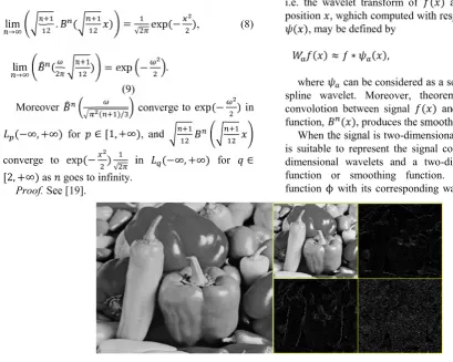
When the signal is two-dimensional, like an image, it is suitable to represent the signal components by two-dimensional wavelets and a two-two-dimensional scaling function or smoothing function. For any scaling functionϕwith its corresponding wavelet , there are

Figure 2.Gaussian (dotted line) and spline (line) (left for n=1 and right for n=3)

three different dimensional wavelets and one two-dimensional scaling function using tensor product approach. We write the two-dimensional wavelets as

( , ) = ( ). ϕ( ), (11)

( , ) = ϕ( ). ( ), (12)

( , ) = ( ). ( ) (13)

and the two-dimensional scaling function as

ϕ( , ) = ϕ( ). ϕ( ). (14)

Based on image decomposition model of wavelet transform, the original image can be divided into four areas. The area which is obtained by convolution between the image and ϕ( , ). This area shows the smoothing image of the original image which contains the most information of the original image. and that preserves the vertical and horizontal edge details respectively, can be computed by convolving the image with ( , ) and ( , ). In the last, one can convolve the image with ( , )to compute who preserves the diagonal details which are influenced by noise greatly. The result can be decomposed as needed. The process for peppers image is shown in Figure 3.

Edge detection

This section explains how we can use wavelet transform for detecting edges in an image. Most multiscale edge detectors smooth the signal at various scales and detect abrupt variation points from their first-or second-derivative. The zero-crossing of the second derivative corresponds to the extrema of the first derivative and the inflection points of the smoothed signal, [10,11]. In section 2, we have showed the smoothed signal could be obtained by convolving signal with B-spline scaling function. Moreover, we have used B-spline wavelets for computing wavelet transform of signal.

In dimensional case, we need to define two-dimensional smoothing and wavelet functions. However, ( , ) is a smoothing function if converges to 0 at infinity and its integral over and is equal to 1. Moreover, we can define two wavelet functions

( , )and ( , )as following

( , ) = ( , ) ( , ) = ( , ). (15)

Now, the image ( , ) can be smoothed by a convolution with ( , ). Then, according to (3), (4) and theorem 2.1, we can obtain the wavelet transform of

smoothed image in the and directions by convolution with ( , )and ( , )respectively,

( , ) ≈ ∗ ( , ), (16)

( , ) ≈ ∗ ( , ). (17)

In other hand, if we denote the smoothed image by

( , ), i.e.

( , ) = ∗ ( , ), (18)

then the gradient vector of ( , )is

∇ ( , ) = ( , ), ( , ) . (19)

Now, we can approximate the gradient vector,

∇ ( , ), by convolving the original image ( , )with

( , )and ( , )as following

( , ) = ( ∗ ( , )) = ∗ ( , ) = ∗

( , ), (20)

( , ) = ( ∗ ( , )) = ∗ ( , ) = ∗

( , ). (21)

So, by equations (16) and (17) we have

∇ ( , ) ≈ ( , ), ( , ) . (22)

If we define the modulus of the gradient vector as the following

( , ) = | ( , )| + | ( , )| , (23)

then we can detect edges of image ( , )by finding modulus maximum points, [12]. Since the edge points are those pixels where the image has sharp intensity variatoin, the information about the direct of this variation is helpful. In geometric concept, the Hessian matrix could be considered as a tool for finding the maximum variation direction, [13,17].

The matrix of second order derivatives of an image at each pixel is called Hessian matrix . In other word, if an image is supposed as a two variable function ( , ), then is

Since taking derivatives of discrete image is an ill-posed operation, we use the wavelet transform of image to approximate the Hessian matrix . In other word, one can compute the Hessian matrix's elements by using equations (11), (12), (13), (20) and (21).

The eigenvector corresponding to the Hessian matrix's largest absolute eigenvalue demonstrates the direction of largest surface curvature. So, we can use this dirction to modify the modulus of gradient vector. Suppose = ( , ), we compute the modulus of the gradient vector by the following formula:

( , ) = | . ( , )| + | . ( , )| . (25)

Infact, we use the Hessian matrix's information to increase or decrease the effect of wavelet transform in and directions. In next section some examples which show the effeciency of our method will be stated.

Results

This section consists of experimental results for a set of standard images. In order to verify the efficiency and accuracy of the proposed algorithm, some images are

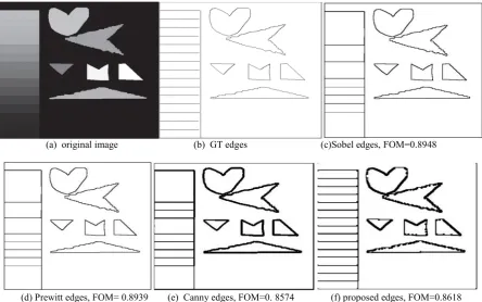
used as experimental subjects. Unlike other common signal-processing applications, such as compression, resizing/interpolation, and filtering (in some cases), there is no ground truth (GT) of the actual edge locations typically known, so comparing the achieved output to an “ideal” is impossible. Thus, one must create the ground truth egdes outlined by hand. In this case, the GT is known, Pratt’s figure of merit (FOM) [20] can be used to compare the edge detection output to the actual edge map. It indicates not only the detected correct edge pixels but also it can determine the accuracy of location with a distance parameter. Figure 4 shows results of the persented method in comparing with Sobel, Prewitt and Canny edge detection methods [4]. The FOM factor of each method is computed for quantitative comparison.

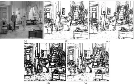
Next, we compare those edge detectors on natural images with more details (Figures 5-8). No ground truth edges are available for quantitative comparison, but visual comparison shows the efficiency of our method.

As we can see from these results, the edges are detected by our method is thinner than those are found by canny method. Moreover, the proposed method detected more correct edge pixels in copmaring with Sobel and Prewitt edge detectors.

(a) original image (b) GT edges (c)Sobel edges, FOM=0.8948

(d) Prewitt edges, FOM= 0.8939 (e) Canny edges, FOM=0. 8574 (f) proposed edges, FOM=0.8618

(a) (b) (c)

(d) (e)

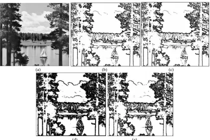
Figure 5.(a) Original Image (b) Prewitt method (c) Sobel method (d) Canny method (e) proposed method

(a) (b) (c)

(d) (e)

(a) (b) (c)

(d) (e)

Figure 7.(a) Original Image (b) Prewitt method (c) Sobel method (d) Canny method (e) proposed method

(a) (b) (c)

(d) (e)

Discussion

In this paper, we proposed an edge detector which obtained by combining wavelet transform based edge detector and Hessian matrix property of images. In fact, we approximated Hessian matrix by wavelet transform. As the experimental results show our algorithm reliable than the traditional ones. The edges of five images were detected to show the efficiency of our method.

References

1. Bishop C.M., Pattern Recognition and Machine Learning. New York, Springer, (2006).

2. Cai X., Chan R., Morigi S., Sgallari F., Vessel Segmentation in Medical Imaging using a Tight-Frame based Algorithm. SIAM, J. Imaging Sciences,6(1): 464-486, (2013).

3. Canny J., A Computational Approach to Edge Detection.

IEEE Transcations on Pattern Anal. and Machine Intelligence,8(6): 679-697 (1986).

4. Gonzalez R.C., Woods R.E. Digital Image Processing, 2nd Ed.. New Jersey, Prentice Hall, (2002).

5. Graaf C. N., Viergever M.A., Information Processing in Medical Imaging. New York: Plenum Press, (1988). 6. Guo W., Lai M-J., Box Spline Wavelet Frames for Image

Edge Analysis. SIAM, J. Imaging Sciences, 6(3): 1553-1578 (2013).

7. Laptev I., Mayer H., Linderderg, T., Eckstein W., Steger C., Baumgarther A., Automatic Extraction of Roads from Aerial Images based on Scale-Space and Snakes. Machine Vision and Applications,12, 23-31 (2000).

8. Mahmoodi S., Edge Detection Filter based on Mumford-Shah Green Function. SIAM, J. Imaging Sciences, 5(1):

343-365 (2012).

9. Mallat S.,A Wavelet Tour of Signal Processing 2nd Ed.. San Diago: Academic Press, (1999).

10. Mallat S., Zero-Crossing of a Wavelet Transform. IEEE Transcations on Information Theory, 37(4):1019-1033 (1991).

11. Mallat S., Hwang W.L., Singularity Detection and Processing with Wavelets. IEEE Transcations on Information Theory,38(2): 617-643 (1992).

12. Mallat S., Zhong S., Charactrization of Signals from Multiscale Edges. IEEE Transcations on Pattern Anal. and Machine Intelligence,14(7): 710-732 (1992).

13. O`Neill B., Elementary Differential Geometry. Academic Press is an imprint of Elsevier (2006) .

14. Russ J., The Image Processing Handbook 2nd Edition. Boca Raton, FL: CDC Press, (1994).

15. Somkantha K., Theera-Umpon N., Auephanwiriyakul S., Boundary Detection in Medical Images Using Edge Following Algorithm Based on Intensity Gradient and Texture Gradient Features. IEEE Transactions on Biomedical Engineering,58(3): 567-573 (2011).

16. Sonka M., Hlavac V., Boyle R., Image Processing, Analysis, and Machine Vision, 3rd Ed.. USA, Thomson, (2008).

17. Staal J., Abramoff M.D., Niemeijer M., Viergever M.A., Ginneken B.V., Ridge-Based Vessel Segmentation in Color Images of the Retina. IEEE Transcations on Medical Imaging,23(4): 501-509 (2004).

18. Szeliski R., Computer Vision: Alghorithms and Applications. New York, Springer (2011).

19. Unser M., Aldroubi A., Eden M., On the Asymptotic Convergence of B-Spline Wavelets to Gabor Functions.

IEEE Transcations on Information Theory,38(2): 864-872 (1992).