The Radiocoloring Problem on Some Graphs

Vol.19, No.2, 2019, 197-206

ISSN: 2279-087X (P), 2279-0888(online) Published on 23 May 2019

www.researchmathsci.org

DOI: http://dx.doi.org/10.22457/apam.618v19n2a9

197

Annals of

The Radiocoloring Problem on Some Graphs

Xiao-ling Zhang

College of Mathematics and Computer Science

Quanzhou Normal University, Quanzhou – 362000, Quanzhou, China E-mail: [email protected]

Received 9 April 2019; accepted 22 May 2019

Abstract. A radiocoloring of a graph G is a function f from the vertex set V G( ) to the set of all non-negative integers (labels) such that | f u( )−f v( ) | 2≥ if d u v( , )=1 and

| f u( )− f v( ) | 1≥ if d u v( , )=2. The number of discrete labels and the range of labels used are called order and span, respectively. In this paper, we concentrate on the minimum order span radiocoloring problem. The optimization problem tries to find, from all minimum order assignments, one that uses the minimum span. We completely determine the minimum order span of paths, cycles and regular lattices. Moreover, we consider some regular bipartite graphs and provide exact value for their minimum order spans.

Keywords: radiocoloring, order, span

AMS Mathematics Subject Classification (2010): 05C15, 05C78 1. Introduction

The frequency assignment problem (FAP) [13] in radio networks is a well-studied, interesting problem, aiming at assigning frequencies to transmitters exploiting frequency reuse while keeping signal interference to acceptable levels. The FAP is, in many cases, studied as a graph coloring problem, in which the vertices represent transmitters, the edges represent interference between two transmitters and the colors represent the frequencies. A radiocoloring, also known as L(2,1)-labeling [11], of a graph G is a function f from the vertex set V G( ) to the set of all non-negative integers (labels) such that| f u( )− f v( ) | 2≥ if d u v( , )=1and| f u( )− f v( ) | 1≥ if d u v( , )=2， whered u v( , )denotes the distance between u and v. The number of discrete labels and the range of labels used are called order and span, respectively.

198

Definition 1.1. (Minimum order RCP) The optimization version of the RCP that tries to minimize the order. The optimal order is called Xorder.

Definition 1.2. (Minimum span RCP) The optimization version of the RCP that tries to minimize the span. The optimal span is called Xspan.

Definition 1.3. (Minimum span order RCP) The optimization version of the RCP that tries to find from all minimum span assignments, one that uses as few labels as possible. The order of such an assignment is called Xorder′ .

Definition 1.4. (Minimum order span RCP) The optimization version of the RCP that tries to find, from all minimum order assignments, one that uses a minimum span. The span of such an assignment is called X_span′ .

It easy to see that Xorder≤Xorder′ and Xorder≤ Xspan+1. Also, it holds that Xspan≤ Xspan′ . The equality holds for graphs of diameter at most two. However, Xspan can be much less

than X_span′ . For example, we can show that X_span( )T = ∆ +2 while X_span′ ( )T = ∆2 , where T is a tree containing a ∆-vertex such that all of its adjacent vertices are ∆-vertex. Another variation of FAP is related to the square of a graph, which is defined as follows: the square 2

G of a graph G is given by 2

( ) ( )

V G =V G and 2

( )

uv∈E G if and only if

( , ) 2

d u v ≤ . The problem is to color the square of a graph G, so that no two adjacent vertices (in 2

G ) get the same color. The objective is to use the minimum number of colors, denoted 2

(G )

χ and called chromatic number of the square of the graph. [9-10] first observed that for any graph G, Xorder is the same as the chromatic number of

2 G ,

i.e. 2

( ) ( )

order

X G =χ G . However, notice that, the set of colors used in the computed assignments of the two problems are different. The colors of the distance one vertices in the RCP should be at frequency distance two instead of one in the coloring of the 2

G . However, from a valid coloring of 2

G we can always reach a valid radiocoloring of G by doubling the assigned color of each vertex. Observe that 2 2

(G ) Xspan( ) 1 2 (G G ) 1

χ ≤ + ≤ χ − .

In [12], it has been proved that the problem of the minimum span RCP is NP-complete, even for graphs of diameter 2. In [16], Lin proved that the problem of coloring the square of a general graph (i.e. the minimum order RCP) is NP-complete. It is also shown that the minimum span order RCP are NP-complete for planar graphs in [9]. To our knowledge, the minimum order span RCP has not been investigated before.

In this paper, we concentrate on the minimum order span radiocoloring problem. The optimization problem tries to find, from all minimum order assignments, one that uses the minimum span. In Section 2, we completely determine the minimum order span of paths, cycles and regular lattices. In Section 3, we consider some regular bipartite graphs and provide exact value for their minimum order spans.

2. The minimum order span of paths, cycles and regular lattices

199 Lemma 2.1. Let G be a graph. Then

(1) ∆ + ≤1 Xorder( ) | ( ) |G ≤V G , and Xorder( ) | ( ) |G =V G if and only if the diameter of G is at most two.

(2) Xspan( )G ≤Xspan′ ( )G , and Xspan( )G =Xspan′ ( )G if the diameter of G is at most two.

(3) [15] 2

( ) ( ) 1

order

X T =χ T = ∆ + , where T is a tree with at least one edge.

In [11], Griggs and Yeh studied the minimum spans of paths and cycles and proved the following results.

Theorem 2.2. [11] Let P_n be a path with n vertices.

Then

2, 2, ( ) 3, 3, 4,

4, 5.

span n

if n

X P if n

if n = 



= =

 _≥



Theorem 2.3. [11] Let C_n be a cycle with n vertices. ThenXspan(Cn)=4.

Now we consider the minimum order span of paths and cycles.

Theorem 2.4. Let Pn be a path with n vertices.

Then

2, 2, ( ) 3, 3, 4, 4.

span n

if n

X P if n

if n = 



′ = =

 _≥



Proof: Let Pn=v v1 2...vn. By Lemma 2.1, it is clear that Xorder(P2)=2 and Xorder(Pn)=3 when n≥3.

For n=2,3, Xspan′ (P₂)=Xspan(P₂)=2 and Xspan′ (P3)=Xspan(P3)=3 using the Lemma 2.1 and the fact that the diameters of P2 and P3 are at most 2.

For n=4, suppose for the contrary, that f is a radiocoloring with order 3 and span 3. If f v( )₂ =1, then { ( ), ( )} {3, 4}f v₁ f v₃ = and f v( )₄ =2, a contradiction to X_order(P₄)=3. If

2

( ) 2

f v = , then { ( ), ( )} {0, 4}f v1 f v3 = . This contradicts the assumption that the span of f is 3. So f v( ) {1, 2}2 ∉ . Similarly, f v( ) {1, 2}3 ∉ . This implies { ( ), ( )} {0,3}.f v2 f v3 = But now { ( ), ( )} {1, 2}f v1 f v4 = , again a contradiction toXorder(P4)=3. Hence Xspan′ (P4)≥4. For n≥5, X_span′ (P_n)≥X_span(P_n)=4 in view of Lemma 2.1 and Theorem 2.2.

For n≥4, in order to show the upper bound, we define a radiocoloring with order 3

and span 4 as follows:

0, 0 (mod 3), ( ) 2, 1 (mod 3), 4, 2 (mod 3).

i

if i

f v if i

if i ≡ 



= ≡

 _≡



200 Theorem 2.5. Let C_n be a cycle with n vertices.

Then ( ) 4, 5 0(mod 3) 0(mod 4),

5, .

span n

if n or n or n

X C

otherwise

= ≡ ≡

 ′ = 

Proof：：：：Let Cn =v v1 2...v vn 1. Observe that Xorder(C5)=5 and Xorder(Cn)=3 if n≡0(mod 3). Otherwise, X_order(C_n)=4 by [3].

It follows from Lemma 2.1 and Theorem 2.3 that Xspan′ (Cn)≥Xspan(Cn)=4. Now we

treat the following two cases to prove.

Case 1: n=5 or n≡0(mod 3) or n≡0(mod 4).

For n=5, it is clear that Xspan′ (C5)=Xspan(C5)=4 since the diameter of C5 is 2. For n≡0(mod 3), in order to prove X′span(Cn)≤4, we define a radiocoloring f with

order 3 and span 4 as follows:

0, 0 (mod 3), ( ) 2, 1 (mod 3), 4, 2 (mod 3).

i

if i

f v if i

if i ≡ 



= ≡

 _≡



For n≡0(mod 4), we construct a radiocoloring f with order 4 and span 4 as follows:

0, 0(mod 4), 3, 1(mod 4), ( )

1, 2(mod 4), 4, 3(mod 4).

i

if i if i f v

if i if i ≡ 

 _≡

 =

≡ 

 _≡



Thus, Xspan′ (Cn)=4 when n=5 or n≡0(mod 3) or n≡0(mod 4).

Case 2: n≠5 and n≠0(mod 3) and n≠0(mod 4).

Suppose to the contrary that Cn admits a radiocoloring f with order 4 and span 4. Without loss of generality, let f v( )1 =0. Then { ( ), ( )} {{2,3},{2, 4},{3, 4}}f v2 f vn ∈ . Case 2.1: { ( ), ( )} {2,3}f v2 f vn = .

Then { ( ), (f v3 f vn−1)} {1, 4}= , a contradiction to Xorder(Cn)=4. Case 2.2: { ( ), ( )} {2, 4}f v₂ f vn = .

Assume that f v( )2 =4, ( )f vn =2. In the case, if f v( ) 13 = , then we need f v( )4 =3,

again a contradiction to Xorder(Cn)=4. This implies that f v( )3 =2, ( )f v4 =0. Going on

this process, we have f v( ₃k+₁)=0, (f v₃k+₂)=4 and f v( 3k+3)=2 , where k=0,1,... .

Therefore, n≡0(mod 3). This contradics to our assumption. Case 2.3: { ( ), ( )} {3, 4}f v2 f vn = .

Suppose that f v( )₂ =4, ( )f vn =3. Then f v( n−1)= f v( )3 =1. Going on this process, we have f v( ₄k+₁)=0, (f v₄k+₂)=4, (f v₄k+₃) 1= and f v( 4k+4)=3, where k=0,1,.... Therefore,

0(mod 4)

n≡ , again a contradiction.

201

We present a radiocoloring with order 4 and span 5 as follows: f v( 3k+1)=0,

3 2

( _k ) 4,

f v ₊ = f v( _3k+3)=2, where k=0,1,... and f v( )_n =5 for n≡1(mod 3); f v( )₁ = f v( )₅ 0

= ,f v( )₂ = f v( )₆ =3, f v( )₃ = f v( ) 1₇ = , f v( )₄ = f v( )₈ =5 and f v( _3k)=0, (f v_3k+1)=3,

3 2

( k ) 5

f v ₊ = , where k=3, 4,..., for n≡2(mod 3).

Therefore,Xspan′ (Cn)=5 when n≠5 and n≠0(mod 3) and n≠0(mod 4).

This concludes the proof of Theorem 2.5. □

In the following, we will consider the minimum order span of regular lattices. The minimum order and span of regular lattices have been proved by means of optimal-labelling algorithms in [3,5] respectively.

Theorem 2.6. [3,5] Let G∆ be a ∆-regular lattice, where ∆ =3, 4 or 6.

Then

4, 3, ( ) 5, 4, 7, 6.

order

if

X G if

if ∆

∆ = 



= ∆ =

 _{∆ =}



For a vertex v V G∈ ( ), let N v( )={ :u uv∈E G( )} andN v[ ]=N v( )∪{ }v .

Theorem 2.7. Let G∆ be a ∆-regular lattice.

Then

6, 3, ( ) 8, 4, 12, 6.

span

if

X G if

if ∆

∆ = 



′ = ∆ =

 _{∆ =}



Proof：：：：In view of X_order(G₄)=5, we assume that f is a radiocoloring with order 5 and

4 1 2 3 4 5

( ( )) { , , , , }

f V G = a a a a a . Let u∈V G( ₄) and ( )f u =ai for some i∈{1, 2,3, 4,5}. Then

1 2 3 4 5

( ( )) { , , , , } \ { }i

f N u = a a a a a a . This implies |aj−ai| 2≥ for each j≠i. In fact, for all

{1, 2,3, 4,5}

i∈ , we always have |a_j−a_i| 2≥ for each j≠i. Hence X_span′ (G₄)≥8. Similarly, we can show thatX_span′ (G₃)≥6 and X_span′ (G₆) 12≥ .

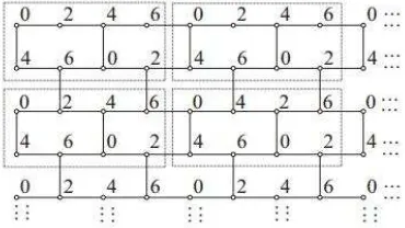
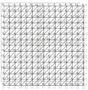
It remains to give a radiocoloring of G₄ with order 5 and span 8, as shown in Figure 1; a radiocoloring of G₃ with order 4 and span 6, as shown in Figure 2. And a radiocoloring of G₆ with order 7 and span 12 is given in Figure 3. This complete the proof of Theorem 2.7. □

3. The minimum order span of some regular bipartite graphs

In this section, we consider the minimum order span of k-regular bipartite graphs on 2n

vertices.

Theorem 3.1. Let G be a k-regular bipartite graph on 2n vertices. If k=n or n−1, then

2 , ,

( ) ( )

2 2, 1.

span span

n if k n

X G X G

n if k n

= 

′ = =

202

Proof：：：：For k=n or n−1, observe that G is a regular bipartite graphs with diameter two. Thus X_span′ ( )G =X_span( )G by Lemma 2.1.

On the other hand, Xspan( )G =2n when k=n, which is shown by Crompton in [7].

For k= −n 1, it is shown by Liu and Yeh [17] that Xspan( )G =2n−2. This completes the

proof of the theorem. □

Figure 1: A radiocoloring of G4 with order 5 and span 8.

Figure 2: A radiocoloring of G3 with order 4 and span 6.

Next, we consider the case for k= −n 2. The following result shows the order of

(n−2)-regular bipartite graph on 2n vertices.

Theorem 3.2. [26] Let Gbe a (n−2)-regular bipartite graph on 2n vertices.

Then

1, 2, ( ) 2, 3, , 4.

order

if n

X G if n

n if n = 



= =

 _≥

203

Figure 3: A radiocoloring of G₆with order 7 and span 12.

Theorem 3.3. Let G be a (n−2)-regular bipartite graph on 2 (n n≥5) vertices. Then

( ) 2( 1)

span

X′ G = n− −l, where l is the number of 4-cycles in K_{n n,} −G.

Proof：：：：Firstly, Xorder( )G =n in view of n≥5. Suppose that {C C1, 2,...,Ck}is the set of all cycles in K_{n n,} −G. Let G=( , )X Y , G_i =G C[ _i]=(X Y_i, )_i , where X_i =V C( _i)∩X Y, _i =V C( _i)

Y

∩ . Let f be a radiocoloring of Gwith order n and f V G( ( i))={ ,a a1 2,...,an}. Then we have the following facts hold.

Fact 1: For each x y, ∈X (or x y, ∈Y ), it must be that d x y( , )=2 since n≥5. Thus all labels in f X( )or all labels in f Y( ) are all different. This means

( ) ( ) ( ( ))

f X = f Y = f V G .

Fact 2: For each x V G∈ ( i),y∈V G( j)(i≠ j), we have d x y( , )=1. Therefore f V G( ( i))∩ f V G( ( j))= ∅ for all i≠ j.

Combined with Fact 1 and Fact 2, we obtain f X( i)= f Y( )i = f V G( ( i)) for each i.

204 On the other hand, suppose 1 1 2 2... i i 1

i i i i i i i

i n n

C =x y x y x y x , where i j

x ∈Xand i j

y ∈Y for

1, 2,..., i

j= n, i=1, 2,...,k. With no loss of generality, let C C1, 2,...,Cl be all the 4-cycles. We define a radiocoloring of G with order n and span 2(n− −1) l as follows.

For i=1, 2,...,l, ( ) ( ) 3 3, 1, 3 2, 2.

i i

j j

i if j f x f y

i if j

− =

 = =

− =



For i= +l 1,...,k, j=1, 2,...,ni, 1

1

(3 2) 2 , _1, ( ) ( )

2,..., . (3 2) 2 2 ,

i i

i

j j

t t l

l j _{if i l}

f x f y

if i l k

l n j

− = + − +  _{= +}  = = = + − + Σ +  Then 1 1 1

( ) ( k) (3 2) 2 2 (3 2) 2 (3 2) 2( 2 ) 2( 1)

k k

k

span _n t k t

t l t l

X G f y l − n n l n l n l n l

= + = +

′ ≤ = − + Σ + = − + Σ = − + − = − − .

Therefore, X_span′ ( )G =2(n− −1) l. □

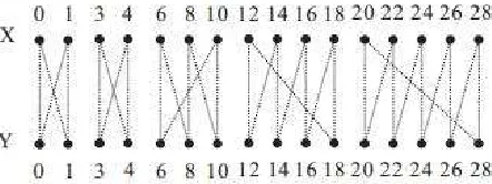
Figure 4: The radiocoloring on a 14-regular bipartite graph on 32 vertices with order 16 and span 28, where K_{n n,} − =G C₁∪C₂∪C₃∪C₄∪C₅ and |C1| |=C2| 4,|= C3| 6,|= C4| 6,|= C5| 10= .

Finally, we consider the minimum order span of incidence graph of a projective plane. We say a graph Gis an incidence graph of a projective plane Π( )n of order n, if

( , , )

G X Y E is a bipartite graph such that

(1) 2

|X| |=Y|=n + +n 1,

(2) each x∈X corresponds to a point p_x in Π( )n and each y∈Y corresponds to a line

y

l in Π( )n , and

(3) E={{ , },x y x∈X y, ∈Y such that px∈ly in Π( )}n .

By the definition of Π( )n , we know that such Gis (n+1)-regular, for every

,

x y∈X , d x y( , )=2, and for every x y, ∈Y, d x y( , )=2. Also, if x∈X y, ∈Ysuch that x is not adjacent to y, then d x y( , )=3.

Theorem 3.4. Let Gbe the incidence graph of a projective plane of order n.

Then 2

( )

span

X′ G =n +n.

Proof：：：：It is shown by Liu and Yeh [17] that 2

( ) ( ) 1

span order

X G = X G + =n +n. Since

2

|X|=n + +n 1 and for every x y, ∈X, d x y( , )=2, for any radiocoloring f of G with span 2

n +n, the order of f is always 2

1

n + +n . Hence 2

( )

span

205

By the definition, we know that the diameter of the incidence graph of a projective plane of order n is 3. However, Xspan′ ( )G =Xspan( )G . This implies the diameter of G is at

most two is sufficient but not necessary for X_span′ ( )G =X_span( )G .

Acknowledgements. This work is supported by the National Natural Science Foundation of China (No. 11601265) and High-level Talent Innovation and Entrepreneurship Project of Quanzhou City, China (No. 2017Z033). The author is also thankful to the reviewers for their valuable suggestion.

REFERENCES

1. S.Amanathulla and M.Pal, L(3,2,1)- and L(4,3,2,1)-labeling problems on interval gra phs, AKCE International Journal of Graphs and Combinatorics, 14 (3) (2017) 205-2 15.

2. S.Amanathulla and M.Pal, Surjective L(2,1)-labeling of cycles and circular-arc grap hs, Journal of Intelligent & Fuzzy Systems, (2018) 1-10.

3. R.Battiti, A.A.Bertossi and M.A.Bonuccelli, Assigning codes in wireless networks: bounds and scaling properties, Wireless Netw, 5 (1999) 195-209.

4. T.Calamoneri, The L(h,k)-labelling problem: an updated survey and annotated bibliography, Comput. J., 54 (2011) 1344-1371.

5. T.Calamoneri and R.Petreschi, L(h,1)-labeling subclasses of planar graphs, J. Parallel Distrib. Comput., 64 (2004) 414-426.

6. G.J.Chang and D.Kuo, The L(2,1)-labeling problem on graphs, SIAM J. Discrete Math., 9 (1996) 309-316.

7. W.Crompton, S.Hurley and N.M.Stephen, A parallel genetic algorithm for frequency assignment problems, in proceedings of IMACS/IEEE International Symposium on Signal Processing, Robotics and Neural Networks (SPRANN’94), Lille, France, April, (1994), 81-84.

8. K.Das, Some algorithm on cactus graphs, Annals of Pure and Applied Mathematics, 2(2) (2012) 114-128.

9. D.A.Fotakis, S.E.Nikoletseas, V.G.Papadopoulou and P.G.Spirakis, Radiocoloring in planar graphs: Complexity and approximations, Theo. Comput. Sci., 340 (2005) 514-538.

10. D.A.Fotakis, S.E.Nikoletseas, V.G.Papadopoulou and P.G.Spirakis, NP-completeness results and efficient approximations for radiocoloring in planar graphs, In: Proceedings of the 25th International Symposium on Mathematical Foundations of Computer Science, Lecture Notes of Computer Science, vol. 1893, pp. 363-372. Springer (2000).

11. J.R.Griggs and R.K.Yeh, Labelling graphs with a condition at distance 2, SIAM J. Discrete Math., 5 (1992) 586-595.

12. J.Griggs and D.Liu, Minimum span channel assignments, Recent advances in radio channel assignments, invited mini-symposium, Discrete Math. (1998).

13. W.K.Hale, Frequency assignment: Theory and applications, Proc. IEEE, 68 (1980) 1497-1514.

206

15. K.W.Lih and W.F.Wang, Coloring the square of an outerplanar graph, Taiwanese J. Math., 10(4) (2006) 1015-1023.

16. Y.L.Lin and S.Skiena, Algorithms for square roots of graphs, SIAM J. Discrete Math., 8 (1995) 99-118.

17. D.D.F.Liu and R.K.Yeh, On distance two labellings of graphs, Ars Combin., 47 (1997) 13-22.

18. S.Paul, M.Pal and A.Pal, L(2,1)-labeling of permutation and bipartite permutation gr aphs, Mathematics in Computer Science, 9 (1) (2015) 113-123.

19. S.Paul, M.Pal and A.Pal, L(2,1)-labeling of interval graphs, Journal of Applied Math ematics and Computing, 49 (1-2) (2015) 419-432.

20. S.Paul, M.Pal and A.Pal, L(0,1)-labelling of Permutation Graphs, Journal of Mathem atical Modelling and Algorithms in Operations Research, (2015) 14-24.

21. P.Pradhan and K.Kumar, The L(2,1)-labeling on propuct of graphs, Annals of Pure and Applied Mathematics, 10(1) (2015) 29-39.

22. S.K.Vaidya and N.B.Vyas, Antimagic labelings of some path and cycle related graphs, Annals of Pure and Applied Mathematics, 3(2) (2013) 119-128.

23. W.F.Wang, The L(2,1)-labelling of trees, Discrete Appl. Math., 154 (2007) 598-603. 24. C.A.Wood and J.Jacob, A complete L(2,1) span characterization for small trees,

AKCE International Journal of Graphs and Combinatorics, 12 (2015) 26-31.

25. R.K.Yeh, A survey on labeling graphs with a condition at distance two, Discrete Math., 306 (2006) 1217-1231.