Crack simulation and probability analysis using irregular truss
structure modeling equivalent to a continuum structure
Won Choi
1,
Seongsoo Yoon
2,
JeongJae Lee
3*(1. Dept. of Rural Systems Engineering, College of Agriculture and Life Sciences, Seoul National University, Seoul 151-921, South Korea; 2. Dept. of Agricultural and Rural Engineering, College of Agriculture, Life and Environments Sciences, Chungbuk National University,
Chungbuk 362-763, South Korea; 3. Dept. of Rural Systems Engineering, Research Institute of Agriculture and Life Sciences, College of Agriculture and Life Sciences, Seoul National University, Seoul 151-921, South Korea)
Abstract: The problems related to agricultural structure engineering for crack simulation and reliability analysis are complicated because its variables contain wide ranges of mean and standard deviation. This paper describes an integrated model to perform crack simulation and reliability analysis of a continuum structure. The structure is assumed to be under a two-dimensional plane stress and the deformation is infinitesimal. A truss structure model that has the same behaviour as a continuum structure was developed using irregular triangle truss components where each element consists of two hinges with an axial degree of freedom at both of their ends. A Monte-Carlo simulation (MCS) was adopted for the reliability analysis. If the length of one side of the irregular triangle mesh is shorter than the thickness of the structure, the slenderness associated with compressive failure needs to be examined only for the short column. For that reason, the failure criterion suitable for the equivalent truss structure model was established by checking only axial stresses acting on truss members. Since nodes of the equivalent truss structure model for the structural analysis in this study consist of hinges, development of plastic hinges that occurred during crack propagation were not considered in this model. To simulate the development of crack, truss members over allowable stresses of tension or compression among truss members with the largest amount of stress at each completed structural analysis time step were sequentially removed. Since irregular triangle meshes have an uncertainty in themselves to compare with regular meshes, the equivalent truss structure model could describe crack propagation more realistically. The failure probabilities of structures under various loads and boundary conditions had good agreement with the analytical solutions directly solved from the limit state equations expressed in the form of moments.
Keywords: crack simulation, probability analysis, irregular truss structure model, failure criteria, Monte Carlo simulation
DOI: 10.3965/j.ijabe.20171001.2024
Citation: Choi W, Yoon S, Lee J. Crack simulation and probability analysis using irregular truss structure modeling equivalent to a continuum structure. Int J Agric & Biol Eng, 2017; 10(1): 234–247.
1 Introduction
Various materials used for constructions of structures
Received date: 2015-06-18 Accepted date: 2016-12-25
Biographies: Won Choi, PhD, Assistant professor, research interests: agricultural engineering applications using multiphysics models and especially agricultural structure engineering, Email: [email protected]; Seongsoo Yoon, PhD, Professor, research interests: agricultural architecture, structural design and automation system, Email: [email protected].
*Corresponding author: JeongJae Lee, PhD, Emeritus professor, research interests: structural and systems engineering. Mailing address: Dept. of Rural Systems Engineering, Research Institute of Agriculture and Life Sciences, College of Agriculture and Life Sciences, Seoul National Univ., 1 Gwanak-ro, Gwanak-gu, Seoul 151-921, South Korea. Tel: +82-2-880-4592, Email: [email protected].
have different probability distributions with regard to
mean and variance of random variables. Particularly,
concrete (mixture of aggregate, sand and cement) has a
relatively wider range of variance than steel[1,2].
Because structure has its own inherent uncertainty,
probabilistic approaches such as structural system
reliability analysis and stochastic structural analysis were
introduced to evaluate structural safety under a variety of
circumstances. Depending on how variables are related
to loads and resistances are handled, current methods can
be classified into the first-order second-moment (FOSM)
method, second-order second moment (SOSM) method,
probabilistic finite element method (PFEM) and
The mean-value first-order second-moment (MVFOSM)
method is based on a first-order Taylor series expansion
of the performance function linearized at the mean values
of the random variables. The failure probability can be
estimated from the reliability index based on the means
(first-order) and variances (second-moment) of the
random variables. However, all variables should follow
a normal distribution and the approach is not invariant
because the failure probability may change depending on
the definition of the limit state equation[4]. The
reliability index geometrically means the shortest distance
from the origin to the failure region[5]. The contact point
on the failure surface is called the most probable failure
point (MPFP)[6,7]. To obtain the MPFP from the
nonlinear limit state equation, the advanced FOSM
(AFOSM) which linearizes the equation around the
MPFP was suggested by introducing iterative methods for
optimization[4]. Because most engineering problems are
related to non-normal distributions, it is necessary to
transform them into normal distributions. If probability
density functions (PDFs) are given, the Rackwitz-Fiessler
equivalent normal transformation can be used[8,9]. The
Rosenblatt transformation is used when joint probability
density functions (JPDF) for random variables can be
transformed into standard normal distributions for
variables[10,11].
Because the FOSM method does not reflect the
curvature characteristics of each limit state equation, the
SOSM method based on a second-order Taylor series
expansion of the performance function linearized at the
mean values of the random variables was introduced[12].
In the most cases, limit state equations could be
approximated by the curvature fitting of second-order
reliability method (SORM)[13-16]. However, the method
could sometimes leave noises on the curvature. In this
case, the point fitted SORM is an alternative[17].
The FOSM and SOSM methods are limited in their
applications because there is no way to know how an
external force applied at a point of a structure affects the
whole system when the structure consists of many
elements. To overcome this weakness, a finite element
method (FEM) was combined with probabilistic
approaches. However, because there is a weakness in
which failure modes associated with limit state equations
are subject to the opinions of designers, the analysis could
produce different results of failure probability.
Therefore, the analysis was mainly applied to simple
structures rather than complex structures[18-20] or static
frame structures in which the materials have less variance
than the components of bulky structures[4,21].
On the other hand, efforts to find dominant failure
modes that affect the entire collapse of a structure have
been ongoing. Ang et al.[22] suggested the basic concept
of failure modes and Ishizawa[23] provided a more rational
basis for determining appropriate safety margins.
Stevenson et al.[24] executed system reliability analysis of
frame structures using the principle of virtual work and
plastic collapse mechanism. Gorman[25] suggested
algorithms to automatically calculate the collapse modes
of perfectly elasto-plastic structures. However, the
applications of these ideas were limited because the
number of failure modes increased exponentially
depending on the degree of structural complexity. Ma
and Ang[26] researched the failure modes of frame
structures and truss structures using nonlinear
programming (NLP), and Moses et al.[27,28] introduced the
incremental loading method (ILM) which would
determine failure modes and limit state equations by
gradually increasing loads. The branch and bound
method to detect the upper bound of failure modes under
a failure event tree was suggested. However, the
method could not handle simultaneous failure modes
because it assumed only gradual failures[29,30]. A β
unzipping method to find failure modes while gradually
removing elements with high failure probability was
developed[30]. This method identified the important
failure modes very quickly but there was always the
possibility of missing out on some important failure
modes. Other researchers developed an optimization
technique using lower bound theory, and the differences
between the upper and lower bound methods were
compared[31]. Simulation based methods[32-35], linear
programming (LP) for detecting failure modes of frame
structures[36], and matrix-based system reliability (MSR)
to find important failure modes by using genetic
Monte-Carlo simulation (MCS) was introduced as an
alternative to PFEM approaches which are limited to only
simple frame structures. The MCS method, which was
developed for nuclear weapon researches in the USA in the 1940’s, creates pseudo-random numbers, simulates
real situations and finds exact solutions. It is a useful
method for those situations where the limit state
equations could not be defined in the PFEM or multiple
integration methods are required due to an excessive
number of probabilistic variables. Most various MCS
approaches are carried out to reduce the number of
iterative calculations. The important sampling method
(ISM) to move the locations of sampling to the boundary
regions between safety and failure was suggested by
Shinozuka[7] and Melchers[38].
Although large-scale complex structures have been
constructed, PFEM as a representative method cannot
give an accurate evaluation of structural safety.
Therefore, additional safety margins are left to the
structures. The equivalent truss structure model
combined with MCS was developed to directly calculate
the failure modes and probabilities, and to significantly
reduce computational time.
2 Mathematical model
The equivalent truss structure model was developed
to substitute solid structure components based on a
continuum mechanism that could not explain failure
phenomena effectively. The basic unit of this model is a
triangular element consisting of three truss elements with
a rotational hinge at both ends of the element. It was
assumed that the mesh density and quality are high
enough to produce a uniform stress distribution within the
triangular domain and to create an equilateral triangle,
respectively.
2.1 Stress and strain relationship of triangular plane element
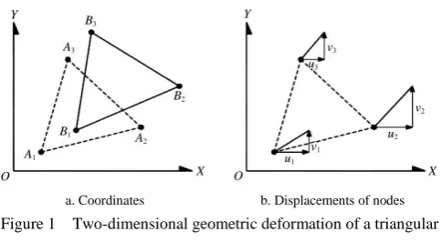
Figure 1a shows the relative locations of the nodes of
a triangular plane element under plane stress before and
after deformation. If the size of the element is
infinitesimal, it can be assumed that the stress distribution
within the domain is uniform. If all sides of the element
maintain a straight line after the element is deformed, all
displacements within the domain will exhibit a linear
relationship between them. Figure 1b shows the
displacements of nodes before and after deformation.
Based upon the linear assumptions, the displacements u
and v can be expressed as:
1 2 3
u a a xa y (1)
4 5 6
va a xa y (2)
where, a1, a2, a3, a4, a5, and a6 are the coefficients; x and
y are the horizontal and vertical directions of the
coordinate system, respectively; u and v are the
displacements of the x- and y-axes, respectively.
a. Coordinates b. Displacements of nodes Figure 1 Two-dimensional geometric deformation of a triangular
solid element exposed to plane stress
Second order approximation as an expression for the
displacements can be used to obtain high quality solutions;
however, first order approximations, the results of which
are accurate enough for the analysis of the in-plane
deformation dealt with in this research, were adopted.
By obtaining the coefficients a2, a3, a5, and a6 as a
form of the coordinates and displacements of nodes 1, 2,
and 3 from Equation (1) and (2), the strain-displacement
relationships can be rewritten as:
1 2 2 3 2 3 1 2
1 2 2 3 2 3 1 2
( )( ) ( )( )
( )( ) ( )( )
x
u u y y u u y y
x x y y x x y y
(3)
1 2 2 3 2 3 1 2
1 2 2 3 2 3 1 2
( )( ) ( )( )
( )( ) ( )( )
y
v v x x v v x x
y y x x y y x x
(4)
1 2 2 3 2 3 1 2
1 2 2 3 2 3 1 2
1 2 2 3 2 3 1 2
1 2 2 3 2 3 1 2
( )( ) ( )( )
( )( ) ( )( )
( )( ) ( )( )
( )( ) ( )( )
xy
u u x x u u x x
y y x x y y x x
v v y y v v y y
x x y y x x y y
(5)
where, x1, y1, x2, y2, x3, y3 and u1, v1, u2, v2, u3, v3 are the x
and y coordinates and displacements of nodes 1, 2, and 3,
respectively.
2.2 Internal energy of a triangular plane element
Assuming that the thickness of the solid structure in
is A, the total internal energy of the element can be
derived as:
2 2 2
2( 2 )
2 1
P x y x y xy
At E
U ε ε νε ε Gγ
ν
(6)
where, UP is the internal energy of the plane element; E is
the Young’s modulus; v is the Poisson’s ratio; G is the shear modulus.
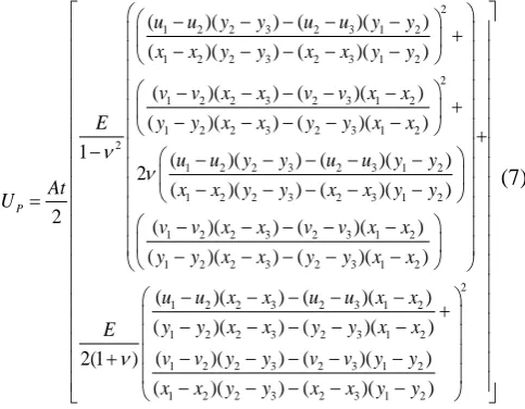
By substituting Equation (6) with Equations (3)-(5),
expressed as the coordinates and displacements of each
corresponding vertex of a triangular plane element, the
total internal energy of the element against the external
forces can be represented as:
2
1 2 2 3 2 3 1 2
1 2 2 3 2 3 1 2
2
1 2 2 3 2 3 1 2
1 2 2 3 2 3 1 2
2
1 2 2 3 2 3 1 2
1 2 2 3 2 3 1
( )( ) ( )( )
( )( ) ( )( )
( )( ) ( )( )
( )( ) ( )( )
1 ( )( ) ( )( )
2
( )( ) ( )(
2
P
u u y y u u y y
x x y y x x y y
v v x x v v x x
y y x x y y x x
E
u u y y u u y y
At x x y y x x y
U 2
1 2 2 3 2 3 1 2
1 2 2 3 2 3 1 2
1 2 2 3 2 3 1 2
1 2 2 3 2 3 1 2
1 2 2 3 2 3 1 2
1 ) ( )( ) ( )( ) ( )( ) ( )( ) ( )( ) ( )( ) ( )( ) ( )( ) ( )( ) ( )( ) 2(1 ) ( y
v v x x v v x x
y y x x y y x x
u u x x u u x x
y y x x y y x x
E
v v y y v v y y
x 2
2)( 2 3) ( 2 3)( 1 2)
x y y x x y y
(7)
2.3 Internal energy of triangular truss element
There exists a triangular truss element that has the
same behaviour as the triangular plane element, as shown
in Figure 2.
When the cross-sectional areas of members of a
triangular truss element are assumed to be A1, A2, and A3,
the internal energy of the element in the state of a
two-dimensional plane stress can be obtained with
following equation:
2 2 2
1 1 1 2 2 2 3 3 3
1 1 1
2 2 2
T
U Eε A Eε A Eε A (8)
where, UT is the internal energy of the triangular truss
element; ε1, ε2, ε3, and A1, A2, A3, and 1, 2, 3
are the deformed strains, and cross-sectional areas, and
lengths of the triangular truss members 1, 2, and 3,
respectively.
Figure 2 Triangular truss element
To determine the relationship between the
cross-sectional area of each member and the weighted
area associated with each member, and to find the
conditions where the discretized truss element has the
same behaviour as the continuum solid element, weighted areas (with regard to their center of gravity ‘G’) are introduced, and the weighted areas (A′1, A′2, and A′3) are
identical to each other. Therefore, the following
relationship can be induced as:
1 2 3
A A A nA (9)
where, n is any multiple.
Figure 3 Weighted areas of triangular truss element
Finally, the internal energy of the triangular truss
element can be obtained by substituting Equation (8) with
the deformed strains of each truss member induced
geometrically from Figure 2.
2
2 2 2 2
2 2 3 3 2 2 3 3 2 3 2 3
1
2 2
2 3 2 3
2
2 2 2 2
1 1 3 3 1 1 3 3 1 3 1 3
2
2 2
1 3 1 3
2
1 1 2 2
( ) ( ) ( ) ( ) ( ) ( )
1
2 ( ) ( )
( ) ( ) ( ) ( ) ( ) ( )
1
2 ( ) ( )
( ) ( ) (
1 2 T
x u x u y v y v x x y y
U E nA
x x y y
x u x u y v y v x x y y
E nA
x x y y
x u x u
E
2 2 2 21 1 2 2 1 2 1 2
3
2 2
1 2 1 2
) ( ) ( ) ( )
( ) ( )
y v y v x x y y
nA
x x y y
2.4 Relationship between continuum and discretized structures
The internal energies of triangular plane (solid
structure) and triangular truss (discretized structure)
elements can be calculated using Equations (7) and (10),
respectively. If the geometries of both structural
elements resisting external forces are deformed in the
elastic range, and both the internal energies have the same
value, it is possible to substitute the solid element with
the discretized element. To apply the equivalence
principle for the internal energies of the solid and
discretized elements, it is necessary to rearrange the
equations in terms of arbitrary variables: displacements u
and v. However, since the displacements of the
triangular truss element in the internal energy equation
are represented as square roots, it is required to continue
to square both sides of the energy equivalence equation
until the square roots disappear.
Because this repeated process to eliminate the square
roots is complicated, the Runge-Kutta method, which is
generally used to find approximate solutions, was adopted
instead. This analysis method found the volume ratio n
that makes the two internal energy equations equal for
any variables u and v under a fixed Poisson’s ratio v. When Poisson’s ratio is 3-1
for ideal materials of isotropic
and homogeneous nature, and 0.2 for materials with a
brittle nature (such as concrete), the volumetric ratios n
were determined to be 2.79036 and 2.79168, respectively.
Because the equivalent truss structure model used in
this study originates from the Laplace equation 2 0,
and the variables belonging to it are governed by a linear
relationship, the regression equation between Poisson’s
ratio (v) and the volumetric ratio (n) should follow a
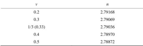
linear relationship. In the regression analysis, the
volumetric ratio and Poisson's ratio showed an exact
linear-relationship, as shown in Table 1.
Table 1 Poisson’s ratio (v) vs. volumetric ratio (n) of the triangular truss element to the triangular solid element
v n
0.2 2.79168
0.3 2.79069
1/3 (0.33) 2.79036
0.4 2.78970
0.5 2.78872
Note: n =–0.00987v+2.79365.
3 Criteria
The model needs to determine special failure criteria
and numerical procedures to apply to crack propagation
and reliability analysis. Detailed explanations of the
model are included in the following sections.
3.1 Loads
Only static loads such as weights loaded on the
surfaces of a rigid body or very slowly moving loads
acting on a sample laid on a universal testing machine
(UTM) for a long time were assumed.
3.2 Tension
Because structural elements generally have material
uncertainties, a safety factor for taking uncertainties of
material into account should be considered. The
allowable stress of an element is given by the following
equation.
allow
c
P
σ n σ n
A
(11)
where, σallow is the allowable stress; n is the safety factor
(safety margin); σ is the internal stress; P is the external
load; Ac is the internal cross section area of the material.
A safety factor was not included in this study because it
made the structural analysis method too complex. It is
also assumed that the characteristics of variables are
given as a type of distribution with average and standard
deviation. When a static tension load is applied to ideal
materials such as steel, for which Poisson’s ratio is 0.3, a
typical stress-strain curve is shown in Figure 4. Each
node of the equivalent truss structure element for
structural analysis in this study already consists of a hinge;
therefore, it is supposed that the structural materials to
resist the tension yield when the internal stresses of the
elements reach a proportional stress limit.
3.3 Compression
If the element loaded axially in compression is a
relatively slender structure, the structural component may
buckle due to bending or lateral deflection before the
internal stress reaches its allowable compressive stress.
To check the slenderness (λ) which refers to the eccentric
ratio between the effective length (l) of a column and the
least radius of gyration (r) of its cross section, it is
necessary to classify the structural members into long and
short columns before applying the criteria for
compression. The slenderness can be expressed by
Equation (12).
k A
λ
r I
(12)
where, k is the effective length factor; A is the cross
sectional area; I is the moment of inertia of the area.
The effective length factor k is 1 because each node of
the equivalent truss structure model consists of a hinge.
If the qualities of irregular triangle meshes consisting of a
whole domain are high enough for three sides of the
triangle meshes to have the same length, the areas of the
triangle meshes can be calculated by Heron’s formula as
follows (Figure 5).
2
3
( )( )( )
4
A s sa sb sc a (13)
where, A' is the area of irregular triangle mesh; s is
( )
2
a b c
and a is the length of one side of the
triangular mesh.
Figure 5 Irregular triangle mesh with side lengths of a, b and c
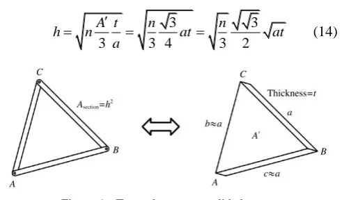
The volume ratio (n) is based on the assumption that
the ratio is the volume of each truss element consisting of
the triangular mesh to the volume of each triangular solid
element divided by the gravity center of the whole solid
element (Figure 6).
If the thickness of the solid element is t and the length
of one side of the sectional area of each truss element is h,
the h can be expressed as follows.
3 3
3 3 4 3 2
A t n n
h n at at
a
(14)
Figure 6 Truss element vs. solid element
Using Equation (14), the slenderness of the equation
(12) can be obtained as follows.
2
3
3 4 3 2
12
3
1 3
12 3 4
n at
A a
λ a
I n n t
at
(15)
The compatibility condition of the equivalent truss
structure model implies that the volume ratio (n) is over 2
(Table 1). If the length (a) of one side of the triangular
mesh is shorter than the thickness (t) of the solid element,
the range of slenderness is given below.
6 45
λ . (16)
3.4 Examination of short and long columns
According to the design criteria of the American
Concrete Institute (ACI), the critical slenderness ratio of a
column not braced against a side sway can be expressed
as follows.
22 u
kl
r (17)
where, lu is the length of the column not braced against
the side sway.
According to the design criteria of the American
Institute of Steel Construction (AISC), the critical
slenderness ratio of a column not braced against a side
sway can be defined as the ratio corresponding to 50% of the yield stress in Euler’s curve when residual stress is considered as shown below.
2
2
c y
k E
r
(18)
where, E is the elastic modulus, MPa and σy is the yield
stress, MPa.
material such as steel with an elastic modulus of 200 GPa
and yield stress of 1000 MPa can be calculated as follows:
35 c
k r
(19)
Therefore, if the structure consists of practical
construction materials such as concrete and steel, the
equivalent truss structure model always satisfies the
conditions of the short column.
3.5 Structural stability
If the global stiffness matrix, which is established by
assembling the local stiffness matrices, has an inverse
matrix while the structural topology is transformed from
stable state to unstable state, the structure is either a
statically indeterminate or determinate structure and there
should be a unique solution to satisfy the relationship
between the global stiffness matrix and the displacements
of nodes. Therefore, the determinant of the structure
can be used as a failure criterion to determine if the
structure will collapse or not.
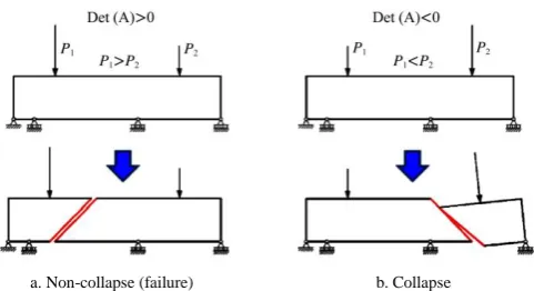
3.6 System collapse
It takes numerous computations to verify the stability
of the collapsing structure by calculating the determinant
of the global stiffness matrix whenever some cracks
propagate during each time step. If the original structure
has various boundary conditions, each structure separated
from the collapsing structure could be an independent
structure depending on some cases such as the situations
shown in Figure 7.
a. Non-collapse (failure) b. Collapse Figure 7 Non-collapse and collapse of statically indeterminate
structure according to load conditions
The designer decides that those independent
structures are statically indeterminate or determinate
structures because the determinants of the structures are
still positive. If there are no induced loads on the
separated structures, the displacements of the structures
will be zero and then the structure will be regarded as
stable.
Therefore, newly defined criteria to determine the
systematic collapse were made on the assumption that the
displacements at some nodes of the original structure are
suddenly larger than the displacements that occurred in
the previous step or become zero.
4 Probability analysis
4.1 Sampling
If the virtual experiments are repeated often enough to
replace the probability variables with a normal
distribution and the structural stability is determined by
checking the limit state equations which define the
collapse conditions of structure, the collapse probability
can be calculated approximately. The Monte-Carlo
sampling technique is a representative method. It is
generally suggested that the total sampling number might
be over 10-100 of the reciprocal of the expected collapse
probability as shown in Equation (20) or should be large
enough to guarantee the accuracy of the expected collapse
probability.
10 to 100
f
N P
(20)
where, N is the total sampling number and Pf is the
collapse probability.
Because the minimum sampling numbers can vary
depending on the situation, such as the shape of the
structure, the condition of the loads and boundary
conditions, the relative errors between previous and
current values of collapse probability were also checked.
4.2 Random variables
It was assumed that the characteristics of variables
related to materials (resistances) and forces (loads)
followed a standard normal distribution. A computer
can produce random numbers from a long sequence that it
creates. These numbers are called pseudo-random
numbers. Because a set of this sequence relies on a
designated number called ‘seeds’ of which the time
corresponds to 1/1000 s, the computer can create different
random numbers as often as desired. To create random
numbers between 0 and 1, the random function embedded
USA) was called out recursively. Box-Muller functions
as shown in Equations (21) and (22) transformed the
random numbers created by the computer into a standard
normal distribution[39].
1/ 2
1 ( 2.0ln( 1)) cos(2 2)
U X X
if X30.5 (21) 1/ 2
2 ( 2.0ln( 1)) sin(2 2)
U X X
if X30.5 (22)
where, U1 and U2 are the non-associated standard normal
random numbers; X1, X2 and X3 are the random numbers
occurring between zero and one.
The targeted normal distribution can be obtained as
shown in Equation (23):
1 2
( or )
X X
X U U (23)
where, X is the targeted normal distribution; μ is the mean
and σ is the standard deviation.
4.3 Progressive elimination method
When external loads act on a structure, internal
stresses occur at components of the structure following
the stress paths produced by external loads. If the
internal stresses are over the yield stresses, the
components collapse and the extra stresses are
redistributed to neighboring components in order to
balance the structure. These processes will continue
until the structure is stable. It is also assumed that the
loads dealt with in this study are static loads which are
gradually increased or relatively constant during the
simulation. Therefore, the progressive elimination
method, which sequentially removes the structural
components with the largest stresses over the allowable
stresses at each time step of the structural analysis, was
adopted. However, if there were no redundant
components to withstand the external loads during the
processes, the structure was regarded as a collapsed
structure. The detailed procedure is shown in Figure 8.
Figure 8 Progressive elimination method
4.4 Expression of removed components
There are two methods of removing structural
components: actually removing the components or
virtually making material properties of the removed
components zero. Generally, the former method allows
control of the input and output files. This approach
occupies a considerable amount of computational time
compared with the computational time needed for
structural analysis. Therefore, the latter method was
chosen to improve computational speed.
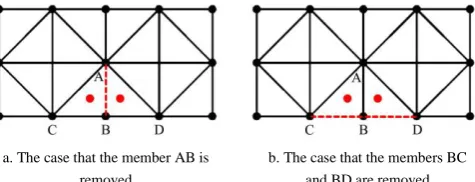
4.5 Removal of unnecessary members as structural components
When truss members with stresses larger than the
yield stress are sequentially removed, truss members
shown to be unnecessary as structural components are
eliminated during the progressive elimination processes.
In Figure 9a, the member AB is removed and the
members BC and BD share the node B; the triangle ACD
is unstable. In Figure 9b, the members BC and BD are
removed; the member AB becomes unnecessary as a
structural component. Therefore, structural analysis at
each time step was carried out after removing all
unnecessary members during the progressive elimination
processes. The rule to remove unnecessary members is
summarized below.
1) Remove any member exceeding the allowable
stresses.
2) Select triangles that share with the member
(triangles including the red dots as shown in Figure 9).
3) Check if there are triangles to share with any
remaining sides of the selected triangles or not. If there
are none, then remove other members connected with the
removed members.
4) Repeat the same elimination processes for all
removed members.
a. The case that the member AB is removed
b. The case that the members BC and BD are removed Figure 9 Unnecessary members as structural components
5 Results and discussion
Beams with various types of loads and boundary
model by executing crack propagation and calculating
failure probability.
5.1 Simply supported beam with a concentrated load
A crack propagation test was conducted, changing the
sizes and triangulation methods of the irregular triangle
mesh. A simply supported beam with a concentrated
load on the top middle point as shown in Figure 10 was
considered for the test.
a
b
c
Figure 10 Crack propagation patterns of the structure using the coarse (a) vs. dense meshes using Delaunay-triangulation-based (b)
and advancing front techniques (c), respectively
The beams had the following characteristics: width of
0.9 m, depth of 1.8 m, span length of 9.0 m, elastic
modulus of 20.0 GPa, concentrated load of 25 kN with
standard deviation of 2 kN, and resisting moment of 60
kN·m with a standard deviation of 6 kN·m. The coarse
meshes consisted of 980 nodes and 2793 elements were
uniformly distributed over the whole domain as shown in
Figure 10a. However, since it is already known that the
crack propagation of the beam occurs at the mid area of
the span, it is possible to increase the mesh density using
dense meshes across the area to reduce the computational
time. For the other beams with different types of mesh
conditions in the area, the whole domain was divided into
9326 elements including 3181 nodes and 14080 elements
including 4782 nodes using Delaunay-triangulation-based
and advancing front techniques, respectively. In the
case of the coarse mesh, the crack developed in the wrong
direction. Even the dense mesh constructed by the
advancing front technique was suboptimal because the
meshes were not distributed consistently through the mid
domain. On the other hand, the case created by the
Delaunay-triangulation-based technique demonstrated
desirable crack propagation.
The failure probability of the structure based on the
Delaunay triangle mesh was calculated as shown in Table
2. An analytical solution for failure probability based on
the limit state equation expressed in the form of a
moment was 30.85% (Thoft-Christensen and Murotsu,
1986). It was understood that the approximate solution
of the failure probability was closer to the analytical
solution as the sampling number increased.
Table 2 Failure probability of simply supported beam under
a concentrated load
Sampling number Failure probability
800 0.2931
2400 0.2974
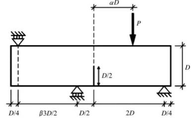
5.2 Crack propagation of a beam subjected to multiple boundary conditions
The experimental result of crack development in
concrete was compared with the regular and irregular
truss structure model equivalent to the continuum[40].
The dimensions and material properties of the structure
subjected to multiple boundary conditions are shown in
Figure 11 and Table 3. In the case of the irregular truss
structure, the region in which the crack occurred was
filled with dense mesh to reduce computational time,
whereas the whole domain of the regular truss structure
was divided into sizes which were equal to the sizes of
the dense meshes of the irregular truss structure. There
were 5611 nodes and 18140 elements, and 1994 nodes
and 5766 elements used for the regular and irregular truss
structures, respectively.
Table 3 Dimensions and material properties of beam
Variables Values Units Description
D 150.00 mm Depth of beam
t 50.00 mm Thickness of beam
L 675.00 mm Span length of beam
α 1.00 Constant
β 1.00 Constant
W 7.50 mm Width of notch
P 13.00 kN Point load
E 38.40 GPa Young’s modulus
v 0.33 Poisson’s ratio
7.50 mm Length of regular truss element
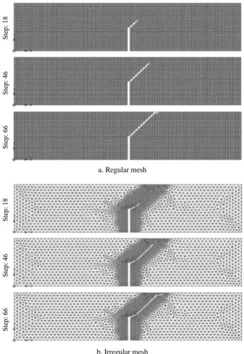
The simulation results of cracks propagated during 66
steps of testing are shown in Figure 12. It took 675 min
and 167 min to complete the crack simulations of the
regular and irregular truss structures, respectively.
a. Regular mesh
b. Irregular mesh
Figure 12 Crack propagations of regular (a) and irregular (b) truss structure models equivalent to continuum
The crack pattern of the regular truss structure was in
a straight line, whereas the crack shape of the irregular
truss structure followed a curvilinear form. The ability
to break away from the main route of the crack was
observed at both the beginning and end times. Research
on fracture mechanism was started by Griffith, and glass
was used for most experiments that included tensile
tests[41,42]. Tensile stress could be a main reason for the
fracture. Brittle materials are fractured in a
trans-crystalline direction, and some cracks changed their
forward direction instantly from the surface of a structure
to the inside. It was also shown in other research that a
fracture in brittle material occurs in the vertical direction
when tensile stresses exist[43]. These observations are in
good agreement with the simulation results of the
irregular truss structure model developed in this study.
5.3 Simply supported beam with two independent concentrated loads
A simply supported beam with two independent
concentrated loads was tested to evaluate the feasibility of
an irregular truss structure model for crack propagation
and probability analysis as shown in Figure 13.
a.
b.
c.
d.
Figure 13 Case that there is no overlapping area between each distribution of two concentrated independent loads; it represents the
locations of loads (a), the possible area of collapse (b), the probabilities of loads (c) and the pattern of crack propagation (d)
The beams had the following characteristics: width of
0.9 m, depth of 1.8 m, span length of 9.0 m, elastic
with standard deviation of 0.37 kN, concentrated load P2
of 21.99 kN with standard deviation of 0.65 kN, and
resisting moment of 60 kN·m with standard deviation of
6 kN·m. The only mid area consisted of a dense mesh
and the whole domain was divided into 6643 elements
including 2260 nodes.
Until the structure collapsed, the crack developed
only at the area subjected to the larger load. The structure’s failure probability was calculated as shown in Table 4. The analytical solution for failure probability
based on the limit state equation expressed in the form of
a moment was 30.85%. The approximate solution to
failure probability was closer to the analytical solution as
the sampling number increased. Therefore, it was
verified that an approach using an equivalent truss
structure model is sufficiently accurate to estimate the
failure probability of the continuum structure.
Table 4 Failure probability when there is no overlapped area between each distribution of two concentrated independent
loads
Sampling number Failure probability
800 0.2861
2400 0.2892
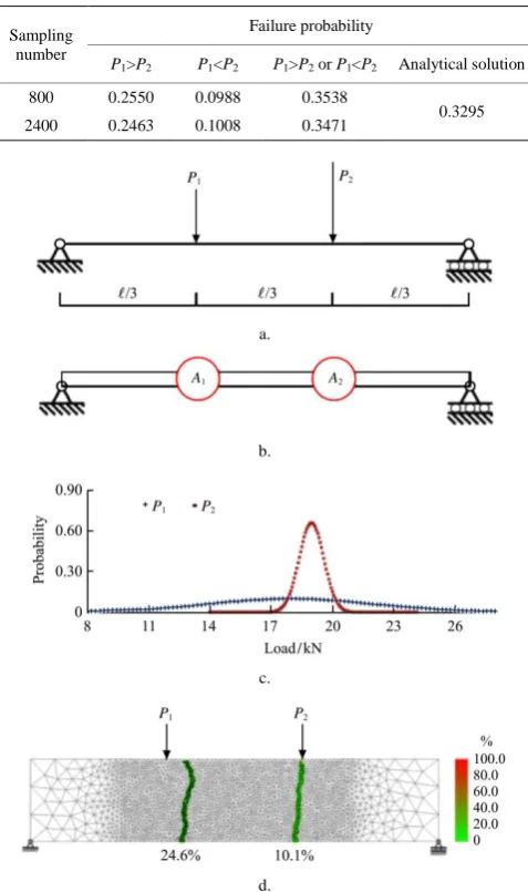
In this time, the special case that the distributions of
the loads P1 and P2 dealt with in the above example were
overlapped by changing the means and standard
deviations of the loads was considered. The loads
included the following details: the concentrated load P1 of
17.97 kN with a standard deviation of 4.00 kN and load
P2 of 18.97 kN with a standard deviation of 0.60 kN. To
obtain the analytical solution for failure probability, the
first conditional case in which load P1 is bigger than load
P2 was assumed (Figures 14 and 15a):
max 1 2
1 1
(2 )
9 9
M PP P (24)
where,
1 2
2
P P P
,
1 2
2 2 2 2
2
P P P
, and Mmax is
the maximum moment that occurs due to the combination
of loads.
The limit state equation could be expressed in the
form of a moment as follows:
max
1 9
R R
gM M M P (25)
where,
9 R
g M P
,
2
2 2 2
9 R
g M P
, and MR
is the resisting moment.
Figure 14 Venn diagram of loads P1 and P2
a.
b.
c.
Figure 15 Various failure modes according to the load conditions: collapses of node 1 (a), node 2 (b), and both nodes 1 and 2 (c) due
to load P1, load P2, and both loads P1 and P2, respectively
The failure probability Pf1 was calculated to be 0.31
from the reliability index β of the limit state equation.
The second conditional case in which the load P2 is
bigger than P1 was assumed (Figures 14 and 15b). The
failure probability Pf2 was calculated to be 0.29 as in the
previous case.
From the Venn diagram shown in the Figure 14, the
failure probability (Pf) of the structure can be set up
following the intersection rule of the Venn diagram.
( ) ( ) ( )
f
P P A P B P AB (26)
From the Figure 14, the probability for only node 1 to
collapse due to the load P1 can be defined as below:.
1 2
( ) f (1 f )
P A P P (27)
The probability for only node 2 to fail due to load P2
can be induced by applying the same method.
1 2
( ) (1 f ) f
P B P P (28)
The probability for nodes 1 and 2 to collapse
1 2
( ) f f
P A B P P (29)
From Equations (26) to (29), the failure probability of
the structure was calculated to be 32.95%. The
simulation results using the equivalent irregular truss
structure model showed that the probabilities were
40.42%, 24.63%, 10.08% and 34.71% in the cases where
the load P1 is greater than P2 without regard to structural
failure; only node 1 collapses due to load P1; only node 2
collapses due to load P2, and nodes 1 or 2 collapse due to
both loads P1 and P2, respectively (Table 5). Two kinds
of failure modes were also observed because the loads
systematically affected each other (Figure 16).
Table 5 Failure probability in the case that there is an overlapped area between each distribution of two concentrated
independent loads
Sampling number
Failure probability
P1>P2 P1<P2 P1>P2or P1<P2 Analytical solution 800 0.2550 0.0988 0.3538
0.3295 2400 0.2463 0.1008 0.3471
a.
b.
c.
d.
Figure 16 Case in which there is an overlapping area between each distribution of two concentrated independent loads; it represents the locations of loads (a), the possible areas of collapse
(b), the probabilities of loads (c) and the patterns of crack propagation (d)
6 Conclusions
A discretized model that shows the same behaviour
as a continuum structure, referred to as the equivalent
truss structure model, was developed based on irregular
triangle elements. With the assumptions that
displacements occurred in a two-dimensional plane, the
deformation maintained a linear relationship, and the
size of the element was infinitesimal enough to have all
stresses at any location inside the domain be identical,
the energy conservation theory was applied to obtain
the necessary conditions for the equivalent truss
structure model. The volumetric ratio of the truss
element to the solid element showed an exact linear
relationship because this model was based on the
Laplace equation. The detailed rules and processes for
the crack propagation and reliability analysis of an
irregular truss structure model were also developed.
Through various examples, it was proved that the
equivalent truss structure model is useful for simulation
of crack propagation and estimating the failure
probability of the continuum structure. The
uncertainty imbedded in the irregular triangle meshes
could describe the propagation of a crack more
realistically. The model could also be expanded for
three-dimensional structure analysis. This model can
be used for the simulations of crack propagation and
reliability analysis in the areas of agricultural
engineering related to structure, soil, food and so on.
However, the model in this study assumes that a crack
propagates statically. Therefore, if the amount of
deformation of a structure exceeds the elastic range
during the crack propagation processes, the crack
propagation model would be inaccurate. Therefore, in
the future, it will be necessary to further develop the
amended model to include the dissipation energy
associated with crack propagation.
Acknowledgment
The work was supported by research grants of
Seoul National University, and Chungbuk National
[References]
[1] Neville A M. Properties of concrete. New York, NY: John Wiley and Sons, 1996.
[2] Park R, Paulay T. Reinforced concrete structures. New York, NY: John Wiley and Sons, 1975.
[3] Corotis R B. Probability-based design codes. Concr. Int., 1985; 7(4): 42–49.
[4] Hasofer A M, Lind N C. Exact and invariant second-moment code format. J. Eng. Mech. Div., ASCE, 1974; 100(1): 111–121.
[5] Cornell C A. Bounds on the reliability of structural systems. J. Struct. Div., ASCE, 1967; 93(1): 171–00.
[6] Freudenthal A M. Safety and the probability of structural failure. T. ASCE, 1956; 121(1): 1337–1397.
[7] Shinozuka M. Basic analysis of structural safety. J. Struct. Div., ASCE, 1983; 109(3): 721–740.
[8] Rackwitz R, Fiessler B. Note on discrete safety checking when using non-normal stochastic models for basic variables. Loads Project Working Session. Cambridge, MA: MIT. 1976.
[9] Rackwitz R, Fiessler B. Structural reliability under combined random load sequences. Comput. Struct., 1978; 9(5): 489–494.
[10] Hohenbichler M, Rackwitz R. Non-normal dependent vectors in structural safety. J. Eng. Mech. Div., ASCE, 1981; 107(6): 1227–1238.
[11] Rosenblatt M. Remarks on a multivariate transformation. Ann. Math. Stat., 1952; 23(3): 470–472.
[12] Fiessler B, Rackwitz R, Neumann H J. Quadratic limit states in structural reliability. J. Eng. Mech. Div., ASCE, 1979; 105(4): 661–676.
[13] Breitung K. Asymptotic approximations for multinormal integrals. J. Eng. Mech. Div., ASCE, 1984; 110(3): 357–366.
[14] Madsen H O, Krenk S, Lind N C. Methods of structural safety. Englewood Cliffs, NJ: Prentice-Hall, Inc. 1986. [15] Tvedt L. Two second-order approximations to the failure
probability. Section on Structural Reliability. Hovik, Norway: A/S Vertas Research. 1984.
[16] Tvedt L. On the probability content of a parabolic failure set in a space of independent standard normally distributed random variables. Section on Structural Reliability. Hovik, Norway: A/S Vertas Research. 1985.
[17] Kiureghian A D, Lin H Z, Hwang S J. Second-order reliability approximations. J. Eng. Mech. Div., ASCE, 1986; 113(8): 1208–1225.
[18] Lee J. Reliability analysis modeling of frame structures based on discretized ideal plastic method. PhD dissertation. Seoul, South Korea: Seoul National University, 1991, 2.
[19] Park S. System reliability analysis of reinforced concrete frames. PhD dissertation. Seoul, South Korea: Seoul National University, 1992, 2.
[20] Yang Y, Kim J. Probabilistic finite element analysis of plane frame. J. Comput. Struct. Eng. Inst. Korea, 1989; 2(4): 89–98.
[21] Handa K, Anderson K. Application of finite element methods in stochastic analysis of structures. Proc. 3rd Intl. Conf. Structural Safety and Reliability. New York, NY: IASAR. 1981.
[22] Ang A H-S, Amin M. Studies of probabilistic safety analysis of structures and structural systems. Urbana, IL: University of Illinois. 1967.
[23] Ishizawa J. On the reliability of indeterminate structural systems. PhD dissertation. Urbana, IL: University of Illinois, 1968.
[24] Stevenson J, Moses F. Reliability analysis of frame structures. J. Struct. Div., ASCE, 1970; 96(11): 2409–2427. [25] Gorman M. Automatic generation of collapse mode
equation. J. Struct. Div., 1981; 107(7): 1350–1354. [26] Ma H-F, Ang A H-S. Reliability analysis of redundant
ductile structural systems. Urbana, IL: University of Illinois. 1981.
[27] Moses F. System reliability developments in structural engineering. Struct. Saf., 1982; 1(1): 3–13.
[28] Moses F, Stahl B. Reliability analysis format for offshore structures. Proc. the 10th Ann. Offshore Technology Conference. Houston, TX: OTC. 1978.
[29] Murotsu Y, Okada H, Taguchi K, Grimmelt M, Yonezawa M. Automatic generation of stochastically dominant failure modes of frame structures. Struct. Saf., 1984; 2(1): 17–25. [30] Thoft-Christensen P, Murotsu Y. Application of structural systems reliability theory. New York, NY: Springer-Verlag. 1986.
[31] Ditlevsen O, Bjerager P. Reliability of highly redundant plastic structures. J. Eng. Mech., ASCE, 1984; 110(5): 671–693.
[32] Grimmelt M, Schueller G I. Benchmark study on methods to determine collapse failure probabilities of redundant structures. Struct. Saf., 1982; 1(2): 93–106.
[33] Melchers R E. Structural system reliability assessment using directional simulation. Struct. Saf., 1994; 16(1-2): 23–37.
[34] Moses F, Fu G. Important sampling in structural system reliability. Proc. the 5th ASCE-EMD/GTD/STD Specialty Conf. Probabilistic Mechanics. Reston, VA: ASCE. 1988. [35] Rashedi M R. Studies on reliability of structural systems.
[36] Corotis R B, Nafday A M. Structural system reliability using linear programming and simulation. J. Struct. Eng., ASCE, 1989; 115(10): 2435–2447.
[37] Kim D. Matrix-based system reliability analysis using the dominant failure mode search method. PhD dissertation. Seoul, South Korea: Seoul National University, 2009, 2. [38] Melchers R E. Structural reliability, analysis and prediction.
West Suxess, England: Ellis Horwood, 1987.
[39] Box G E P, Muller M E. A note on the generation of random normal deviates. Ann. Math. Stat., 1958; 29(2): 610–611.
[40] Gálvez J C, Elices M, Guinea G V, Planas J. Mixed mode fracture of concrete under proportional and nonproportional loading. Int. J. Fracture, 1998; 94(3): 267–284.
[41] Griffith A A. The phenomena of rupture and flow in solids. Philos. T. R. Soc. Lond., 1920; 221: 163–198.
[42] Griffith A A. The Theory of rupture. Proc. 1th Intl. Congr. Applied Mechanics. New York, NY: John Wiley & Sons, Inc, 1924.