Analytical solution of system of differential equations by variational iteration method

(1)

BIBECHANA

A Multidisciplinary Journal of Science, Technology and Mathematics ISSN 2091-0762 (Print), 2382-5340 (0nline)

Journal homepage: http://nepjol.info/index.php/BIBECHANA

Publisher: Research Council of Science and Technology, Biratnagar, Nepal

Analytical solution of system of differential equations by variational

iteration method

Jamshad Ahmed1*, Faizan Hussain2, 3

1

Department of Mathematics, Faculty of Sciences, University of Gujrat, Pakistan

2

Department of Mathematics, University of Gujrat, (Sialkot Campus) Pakistan

3

Department of Mathematics, NCBA&E, Gujrat (Sub-Campus) Pakistan

*

Email:[email protected]

Article history: Received 11 March, 2015; Accepted 17 September, 2015 DOI:http://dx.doi.org/10.3126/bibechana.v13i0.13394

Abstract

In thispaper, Varitational Iteration Method using He’s Polynomials is used to construct the exact as well

as approximate solutions of differential equations. From the obtained numerical results, it has been

observed that this proposed technique is very efficient and reliable for the solution of the linear and

non-linear system of differential equations. Numerical results and graphical representation reflect the accuracy and effectiveness of the proposed modification.

Keywords: Variational interation method; He’s Polynomials; System of linear and non-linear differential equations.

1. Introduction

In recent years considerable interest in system of ordinary differential equations has been stimulated due

to their numerous applications in the fields of physics and engineering. A huge number of research and

investigations have been invested in these directions. In this paper we consider a very efficient and power

full technique He’s variational iteration method for finding approximate solutions of systems of

differential equations. This technique was first time introduce by the Chinese mathematician He [1]. The

variational interaion method is used to investigate autonomous ordinary differential systems [2],

Helmholtz equation [3], Burger’s and coupled Burger’s equation [4], Coupled Schrodinger-KdV equations and shallow water equations [4]. Also the application of the present technique to linear

fractional partial differential equations arising from fluid mechanics is presented in [5]. The variational

(2)

applied to find the solution of various classes of variational problem [11]. Some recent research works in

this field are [12-20].

2. Analysis of VIM for System of Differential Equations In case of m equations, we rewrite equations in the form

,

2 ,

1 ,

)

(

)

(

)

(

y

N

y

₁

y

₂

y

f

x

i

m

L

_i _i



_i







_m



_i





(1)

where

L

iis a linear with respect to

y

iand

N

iis the nonlinear part of ith equation. In this case the correct

functional are obtained as

 

,



 





~

 

,

~

 

,

~

 



 



,

0

, ,

2 , 1 ,

1

, 











x

n m n

n i i

i i

n i n

i

x

y

x

L

y

N

y

f

d

y









(2)

and the optimal values of



_i

,

i



1 ,

2 ,



,

m

,

are obtained by taking the variation from both sides of the functional and finding stationary condition using

. , , 2 , 1 , 0

1

, i m

y_i _n_    

Our goal in the paper is the use of the following system of sequences instead of the system which results

from the Variational iteration method:

 

,



 





 

,

 

,

 



 



,

0

, ,

2 ,

1 ,

1

, 











x

n m n

n i i

i i

n i n

i

x

y

x

L

y

N

y

f

d

y









(3)

For i2,,m. In fact the updated values y1,n1,y2,n2,,y_i1_{ },n1_,are used for finding yi,n1.This

technique accelerates the convergence of the system of sequences. Therefore, using just few terms of the

sequences, an accurate solution can be obtained for a large domain of the problem.

3.Analysis of VIM using He’s Polynomials

Variational Iteration Method using He’s polynomials [21] is a modified form of VIM. This modification

is obtained by coupling the correction functional of VIM with He's polynomials and is given by

 

_{ }

 

_{ }

m i

d f y N p y

L p x p

x y x y

p in in i

n n n

i i n

n x

i i

n

n i n

, , 2 , 1 , ~

, , ,

0 , 0

0 0

, 0

1

,   

  

 

 





_





 

 

  



By comparing the like powers of p, give solution of various order.

4. Numerical Applications

Example 4.1 Consider the system of first order differential equations,

,

cos

3

1

y

x

y







(4)

,

3 2

x

e

y

(3)

,

2 1

3

y







(6)

subjected to the initial conditions

 

0 1,

1 

y y2

 

0 0,

y

3

 

0 

2 .

Accor di n g t o V IM , cor r ect i on f unct i onal f or Eq. ( 4) , ( 5) & ( 6) can be wr i t t en as,

 

   

    

 

   

 

  



   

 

  



   

 

  





  

, ~

~ ,

) ( ) (

, ~

~ ,

) ( )

(

, ~ cos ~

,

, 2 , 1 , 3 0

3 ,

3 1

, 3

0

, 3 , 2 2

, 2 1

, 2

0

, 3 ,

1 1

, 1 1

, 1

 

 

 

 

  

 





d y y d

y d x x

y x y

d e y d

y d x x

y x y

d y

d y d x x

y x y

n n n x

n n

x

n n n

n

x

n n

( 7)

The Lagrange multiplieri

 

x, ,i1,2,3 can be identified via variational theory; i.e. the multiplier should be chosen in such a way that the correction functional equation is stationary i.e.

 

0 ,

₂_, ₁

 

0 &

₃_, ₁

 

0 .

1 ,

1 

x



y



x



y



x



y

_n



_n



_n



From Eq. (7)

 

,

1 ,

1









x



₂

 

x

,







1 ,

and



₃

 

x

,







1 ,

Thus Eq. (7) becomes

 

,

1 )

( ) (

1 )

( )

(

cos )

1 (

, 2 , 1 , 3 0

, 3 1

, 3

0

, 3 , 2 ,

2 1

, 2

0

, 3 ,

1 ,

1 1

, 1

   

    

 

   

 

  

 

   

 

  

 

   

 

  

 



  

 

  



d y y d

y d x

y x y

d e y d

y d x

y x y

d y

d y d x

y x y

n n n x

n n

x

n n n

n

x

n n

(8)

forn0,Eq. (8) gives,

 

    

  

 

, 2

, 1

, sin 1

0 , 3

0 , 2

0 , 1

x y

e x y

x x

y

x

(4)

 

   

    

 

   

 

  

 

   

 

  

 

   

 

  

 



, 1

) ( ) (

, 1

) ( )

(

, cos

) 1 (

0 , 2 0 , 1 0 , 3 0

0 , 3 1

, 3

0

0 , 3 0 , 2 0

, 2 1

, 2

0

0 , 3 0

, 1 0

, 1 1

, 1

 

  



d y y d

y d x

y x y

d e y d

y d x

y x y

d y

d y d x

y x y

x x x

(9)

 

     

 

 

, , sin

2 , 3

2 , 2

2 , 1

x x

e x Cos x y

x x

y

e x y

Therefore, we get the result as,

 

    

 

 

, , sin

3 2 1

x x

e x Cos x y

x x

y

e x y

This is the same result obtained by ADM in [22].

Example 4.2 Consider the non-linear system of differential equations,

,

2

₂2

1

_y

x

d

y

d

_

(10)

,

1 2

_e

_y

x

d

y

d



x

(11)

,

3 2 3

_y

x

d

y

d

_

_

(12)

subjected to the initial conditions

 

0

1 ,

1



y

2

 

0 

1 ,

y

3

 

0 

0 .

The exact solution is given,

y

₁



e

2x

,

y

₂



e

x

,

and y₃xex.

Accor di n g t o V IM , t he cor r ect i on f unct i onal f or t he Eq. ( 10) , ( 11) & ( 12) can be

(5)

 

                                      



    , ~ ~ , ) ( ) ( , ~ , ) ( ) ( , ~ 2 , , 3 , 2 , 3 0 3 , 3 1 , 3 0 , 1 , 2 2 , 2 1 , 2 0 2 , 2 , 1 1 , 1 1 , 1               d y y d y d x x y x y d y e d y d x x y x y d y d y d x x y x y n n n x n n x n n n n x n n n n (13)

The Lagrange multiplier i

 

x, ,i1,2,3can be identified via Variational Theory; i.e. the multiplier should be chosen in such a way that the correction functional equation is stationary i.e.

 

0 ,

₂_, ₁

 

0 &

₃_, ₁

 

0

1 ,

1 

x



y



x



y



x



y

_n



_n



_n



So from Eq. (13), we get

 

,

1 ,

1









x



₂

 

x

,







1 ,

and



₃

 

x

,







1 ,

 

   

 

                                         



    , 1 ) ( ) ( , 1 ) ( ) ( , 2 1 , 3 , 2 , 3 0 , 3 1 , 3 0 , 1 , 2 , 2 1 , 2 0 2 , 2 , 1 , 1 1 , 1         d y y d y d x y x y d y e d y d x y x y d y d y d x y x y n n n x n n x n n n n x n n n n (14)

Accor di n g t o V IM H P, Eq. ( 14) ca n be wr i t t en as

(6)

Now, comparing the co-efficient of like powers of p,  

 

,

0

1

1 :

0 , 3 0 , 2 0 , 1 0













x

y

x

y

x

y

p

 

   

 

   

 

,

)

1 (

1

2

1 :

0 0 , 3 0 , 2 0 , 3 1 , 3 0 0 , 1 0 , 2 1 , 2 0 2 0 , 2 0 , 1 1 , 1 1

































































d

y

d

y

d

x

y

d

y

e

d

y

d

x

y

d

y

d

y

d

x

y

p

x x x

 

,

1

2 :

1 , 3 1 , 2 1 , 1



















x

y

e

x

y

x

y

x  

 

,

2

1

2

4

4 :

2 2 , 3 2 2 , 2 2 , 1 2





























   

x

e

x

y

e

x

e

x

y

e

x

y

p

x x x x  

 

,

6

2

4

2

8

3

12

10

15 :

3 2 2 3 , 3 2 3 , 2 2 3 , 1 3





























       

x

e

x

e

x

y

e

x

e

x

y

e

x

e

x

y

p

x x x x x x x x

Therefore, approximations to the solutions with the five terms are as follows:

  







 













  















































        

3888

.

10 6666

.

4 0083333

.

0 111111

.

0

5 .

7

2

3

12 ,

5555

.

11

13

12 111111

.

0

5

2

8

7

8

4

888 .

134 6666

.

58 11111

.

3

15

6

4

31

26

4

2 5 3 2 3 3 2 2 3 2 2 1

x

e

x

e

x

y

e

x

e

x

e

x

y

x

e

x

e

x

y

x x x x x x x x x

(7)

Table1. Numerical values of these solution.

i

x

y

₁

 

x

_i

e

y

₁

 

x

_i

y

₂

 

x

_i

e

y

₂

 

x

_i

y

₃

 

x

_i

e

y

₃

 

x

_i

0 1.00008 0 1 0 0 0

0.1 1.22132 1.6535E-5 1.10516 2.9323E-6 0.110517 0

0.2 1.49186 5.3375E-5 1.22139 1.1211E-5 0.244275 0

0.3 1.82161 5.9740E-4 1.34974 1.1407E-4 0.404906 5.1165E-5

0.4 2.22249 3.1315E-3 1.49125 5.7298E-4 0.594560 2.7328E-4

0.5 2.70702 1.1341E-2 1.64676 1.9591E-3 0.823372 9.8853E-4

0.6 3.28813 3.2068E-2 1.81686 5.2497E-3 1.090460 2.8076E-3

0.7 3.97860 7.6660E-2 2.00184 1.1909E-2 1.402860 6.7609E-3

0.8 4.79050 6.6253E-1 2.20161 2.3929E-2 1.766030 1.1440E-2

0.9 5.73528 3.1445E-1 2.41576 4.3841E-2 2.185680 2.7962E-2

Graphical representation:

Fig. 1: Comparison of exact and approximate solution of

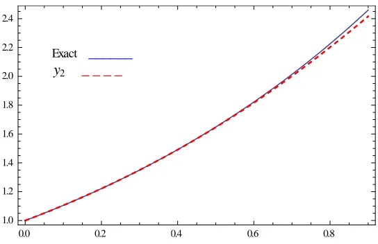
y1,

Fig. 2: Comparison of exact and approximate solution of

y₂_,

Exact ______

y1 _ _ _ _ _

0.0 0.2 0.4 0.6 0.8 1

2 3 4 5

Exact ______

y2 _ _ _ _

0.0 0.2 0.4 0.6 0.8

(8)

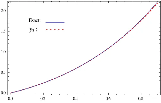
Fig. 3: Comparison of exact and approximate solution of y

3.

Example 4.3 Consider a non-linear ordinary differential equation

,

1

3 3

x

d

y

d

y

x

d

y

d





(16)

subject to the boundary conditions

 

0 0,

y y

 

0 1, y

 

0 2.

Considering y₁

   

x y x , y₂

 

x y

 

x , and

y

3

   

x



y



x

,

we convert Eq. (16) in the system of non-linear of three differential equation of order one, i.e.

 

2

 

,

1 x y x

y  (17)

   

₃

,

2

x

y

x

y





(18)

 

1 ₁

 

₃

 

,

3 y x y x x

x

y   (19)

Accor di n g t o V IM , t he cor r ect i on f unct i onal f or t he Eq. ( 17) , ( 18) & ( 19) can be

wr i t t en as,

 

   

    

 

   

 

 

 

   

 

 



   

 

 





  

, ~

~ 1 ,

) ( )

(

, ~

, )

( )

(

, ~

,

, 3 , 1 ,

3 0

, 3 1

, 3

0

, 3 , 2 ,

2 1

, 2

0

, 2 ,

1 ,

1 1

, 1

 

  

 

 

 



d y y d

y d x x

y x y

d y d

y d x x

y x y

d y d

y d x x

y x y

n n n

x

n n

x

n n n

n

x

n n

( 20) Exact: ______

y3:

-0.0 0.2 0.4 0.6 0.8

(9)

The Lagrange multiplieri

 

x, ,i1,2,3 can be identified via variational theory. i.e. the multiplier should be chosen in such a way that the correction functional equation is stationary i.e.

 

0 ,

₂_, ₁

 

0 &

₃_, ₁

 

0

1 ,

1 

x



y



x



y



x



y

_n



_n



_n



So from Eq. (20), we get

 

,

1 ,

1









x



₂

 

x

,







1 ,

and



3

 

x

,







1 ,

 

   

 

   

    

 

   

 

 

  

   

 

 

 

   

 

 

 



  

, ~

~ 1 1

) ( )

(

, ~

1 )

( )

(

, ~

1

, 3 , 1 ,

3 0

, 3 1

, 3

0

, 3 , 2 ,

2 1

, 2

0

, 2 ,

1 ,

1 1

, 1

 



 



d y y d

y d x

y x y

d y d

y d x

y x y

d y d

y d x

y x y

n n n

x

n n

x

n n n

n

x

n n

(21)

Therefore, we get,

 

    

  

, 2

, 1

, 0

0 , 3

0 , 2

0 , 1

x y

Let

y

r



y

₁_,₀



y

₁_,₁



y

₁_,₂







y

₁_,_r is a notation for an approximation to the solution with p+1 term.

Therefore, some computed approximations are as follows

, 3 1

2 3

   

 

 

x x x

y

, 12 2 1

3 2 4

   

 

  

x x x x

y

, 60 6 2 1

4 3 2 5

   



 _ _ _ _

x x x x x

y

.

,

360

180

7

6

2

1

5 4 3 2 6















_



x

y

The closed form solution is

 

x

e

x

.

y



₍₂₂₎

(10)

4. Conclusion

In this paper, Variational Iteration Method using He’s polynomials has been implemented successfully to

find exact and approximate solutions of linear and nonlinear system of ordinary differential equations.

Three numerical examples have been presented to show that this technique is promising. All the

calculations are performed easily. Therefore, this method can be applied to many other complicated

nonlinear systems of ODEs and PDEs.

References

[1] J. H. He, International Journal of Modern Physics B, 20 (10) (2006) 1141–1199. [2] J. H. He, Applied Mathematics and Computation, 114 (2000) 115–123.

[3] S. Momani, S. Abuasad, Chaos, Solitons and Fractals, 27 (2006) 1119–1123.

[4] M.A. Abdou, A.A. Soliman, Journal of Computational and Applied Mathematics, 181 (2005) 245–251. [5] S. Momani, Z. Odibat, Physics Letters A, 355 (2006) 271–279

[6] M. Dehghan, F. Shakeri, Communications in Numerical Methods in Engineering, (2008) (in press).

[7] A. Saadatmandi, M. Dehghan, Computers and Mathematics with Applications, 58 (11–12) (2009) 2190–

2196.

[8] O. Kıymaz, Int. J. Contemp.Math. Sciences, (5) (37) (2010) 1819–1826. [9] M. Dehghan, A. Saadatmandi, Chaos, Solitons and Fractals, (2008) (in press).

[10] S.A. Yousefi, A. Lotfi, M. Dehghan, Computers and Mathematics with Applications, 58 (11–12) (2009) 2172–2176.

[11] S.A. Yousefi, M. Dehghan, International Journal of Computer Mathematics, (2008) (in press).

[12] A.M. Wazwaz, Central European Journal of Engineering, 4(1) (2014) 64-71.

[13] A. Neamaty and R. Darzi, Boundary Value Problems 2010, 2010: 317369

DOI:10.1155/2010/317369

[14] H. Ozer, International Journal of Nonlinear Sciences and Numerical Simulation, 8 (2007) 513–518.

[15] J. Biazar, H. Ghazvini, International Journal of Nonlinear Sciences and Numerical Simulation, 8 (2007) 311–

314.

[16] Z.M. Odibat, S. Momani, International Journal of Nonlinear Sciences and Numerical Simulation, 7 (2007)

27–34.

[17] J. Ahmad, and S. T. Mohyud-Din, Bibechana, (12) (2015) 59-69,

[18] M. Dehghan, F. Shakeri, New Astronomy, 13 (2008) 53–59.

[19] G.Y Wang, J. H. He, L.F. Mo, LETTER, Lat. Am. J. Solids Struct., 11 (2) (2014).

[20] J. Ahmad, I. Ahmad and B. Ahmad, 21 ( 2013) 1-15.

[21] S. T. Mohyud-Din and M. A. Noor, J. Appl. Math. Comp., (2008)

DOI: 10.1007/s12190-008-0212-7