www.clim-past.net/10/1145/2014/ doi:10.5194/cp-10-1145-2014
© Author(s) 2014. CC Attribution 3.0 License.
Model–data comparison and data assimilation of mid-Holocene
Arctic sea ice concentration
F. Klein1, H. Goosse1, A. Mairesse1, and A. de Vernal2
1Université catholique de Louvain, Earth and Life Institute, Georges Lemaître Centre for Earth and Climate Research,
Place Louis Pasteur, 3, 1348 Louvain-la-Neuve, Belgium
2GEOTOP, Université du Québec à Montréal, P.O. Box 8888, succursale “centre ville”, Montréal, QC H3C 3P8, Canada
Correspondence to: F. Klein ([email protected])
Received: 15 November 2013 – Published in Clim. Past Discuss.: 10 December 2013 Revised: 3 April 2014 – Accepted: 15 April 2014 – Published: 16 June 2014
Abstract. The consistency between new quantitative recon-structions of Arctic sea ice concentration based on dinocyst assemblages and the results of climate models has been in-vestigated for the mid-Holocene. The response of the models mainly follows the increase in summer insolation, modulated to a limited extent by changes in atmospheric circulation. This leads to differences between regions in the models that are smaller than in the reconstruction. It is, however, impos-sible to precisely assess the models’ skills because the sea ice concentration changes at the mid-Holocene are small in both the reconstructions and the models and of the same order of magnitude as the reconstruction uncertainty. Performing sim-ulations with data assimilation using the model LOVECLIM amplifies the regional differences and improves the model– data agreement as expected. This is mainly achieved through a reduction of the southward winds in the Barents Sea and an increase in the westerly winds in the Canadian Basin, in-ducing an increase in the ice concentration in the Barents and Chukchi seas. This underlines the potential role of atmo-spheric circulation in explaining the reconstructed changes during the Holocene.
1 Introduction
Sea ice is a key element of the global climate system. First, it enhances climate response at high latitudes of the Northern Hemisphere as it is involved in various feedbacks, in partic-ular the classic ice albedo feedback (Holland and Bitz, 2003; Serreze et al., 2009; Screen and Simmonds, 2010; Stroeve et al., 2011). Second, sea ice plays a role in deep-water for-mation through brine rejection which is a crucial driver of
the global thermohaline circulation (Lohmann and Gerdes, 1998; Goosse and Fichefet, 1999). Third, it modifies the ex-changes of heat and gases between the atmosphere and polar oceans because of its insulation properties (Ebert and Curry, 1993). Consequently, changes in Arctic sea ice cover and thickness influence the atmospheric and hydrographic con-ditions at high latitudes, which may in turn have an impact on the European and the North American climate (e.g. Ser-reze et al., 2007; Francis and Vavrus, 2012).
Here we will focus on the mid-Holocene (6 ka, hereafter MH) as it is a classic period that is reasonably well docu-mented as much in terms of proxy data (see Sect. 3.1) as in terms of model results since it is a standard target for the Paleoclimate Model Intercomparison Project (PMIP; e.g. Braconnot et al., 2007). The MH coincides with the end of a warm period in the Arctic that started about 9 ka (Sundqvist et al., 2010) due to a high orbitally driven summer insolation. Insolation had its maximum at around 11 ka (Berger, 1978) but the warmest conditions have been asynchronous across the Arctic due to the effect of the lingering Laurentide Ice Sheet (Kaufman et al., 2004; Renssen et al., 2009). At 6 ka, some regions were thus already experiencing a cooling (for instance, Alaska) while others were still close to their max-imum temperature (like northeast Canada) (Kaufman et al., 2004).
Although most Arctic proxies support lower sea ice con-ditions during the MH as compared to the entire Holocene, the recorded changes are not homogeneous between the dif-ferent regions (see Sect. 3.1). In addition to modifications in the oceanic and atmospheric circulations or to the influence of the remnant Laurentide Ice Sheet that could have an im-pact on a large scale, complex local topography can be re-sponsible for a high heterogeneous response on small spatial scales. This is particularly the case in the Canadian Arctic Archipelago (CAA) with its complicated disposition of nar-row straits, where proxy records display contrasted signals for nearby locations (e.g. Vare et al., 2009; Atkinson, 2009). Furthermore, the uncertainties related to the interpretation of proxies or to their dating can also explain some of the dis-crepancies (Polyak et al., 2010; Sundqvist et al., 2010).
In qualitative agreement with data, models simulate less sea ice extent in summer during the MH as compared to the pre-industrial (hereafter PI) conditions, following the higher summer insolation (Berger et al., 2013; Goosse et al., 2013). However, no quantitative estimate of the agreement exists up to now, given the lack of a consistent quantitative sea ice re-construction covering the Arctic. In this context, this paper aims at comparing the MH sea ice concentration simulated by the model of intermediate complexity LOVECLIM and by general circulation models (GCMs) with new quantita-tive reconstructions of Arctic sea ice concentration based on dinocyst assemblages (de Vernal et al., 2013a). This model– data comparison is intended first to estimate whether climate models are able to reproduce the spatial pattern deduced from proxy records. In a second step, a simulation with data as-similation is performed with the climate model LOVECLIM. The data assimilation method is constructed in such a way that the impact of this additional constraint improves the con-sistency between the model results and the reconstruction. This allows us to investigate in more details the processes governing sea ice conditions at 6 ka and analysing the poten-tial origin of the biases seen in the simulations without data assimilation.
The models selected, the experimental design and the proxy reconstructions based on dinocyst assemblages are presented in Sect. 2. Section 3 starts with a short description of the observed sea ice changes. It is followed by an analysis of the results of the simulations without data assimilation and finally of the simulation with data assimilation. Conclusions are presented in Sect. 4.
2 Methodology 2.1 Model description
Experiments have been performed with the three-dimensional earth climate model of intermediate complexity LOVECLIM version 1.2 (Goosse et al., 2010). It includes a representation of the atmosphere, ocean, sea ice and land surface including vegetation. The atmospheric component is ECBilt2 (Opsteegh et al., 1998), a quasi-geostrophic spectral model with T21 horizontal resolution (correspond-ing to 5.6◦×5.6◦ latitude–longitude) and three vertical levels in addition to the surface. Ocean and sea ice are simulated by CLIO3 (Goosse and Fichefet, 1999), which is a general circulation model coupled to a comprehensive thermodynamic–dynamic sea ice model. Its horizontal resolution is 3◦×3◦ and the ocean is divided into 20 un-evenly spaced vertical levels. LOVECLIM also contains the vegetation model VECODE (Brovkin et al., 2002) that takes into account the distribution of three different land covers (deserts, grasses and forests) using the same resolution as ECBilt2. Due to its coarse resolution and to simplifications introduced in the representation of some atmospheric processes, LOVECLIM is much faster than the more sophisticated coupled climate models. It allows us to produce the large amount of simulations required for the data assimilation process (see Sect. 2.2). In this study, two different 6 ka LOVECLIM simulations are examined: LOVECLIM without assimilation (referred as LOVECLIM no assim) and LOVECLIM with sea ice data assimilation (LOVECLIM assim SIC).
In addition to LOVECLIM simulations, MH experiments performed with GCMs in the framework of the third phase of the PMIP3 (Otto-Bliesner et al., 2009), referred to as
mid-Holocene, are analysed. The simulations from which the PI
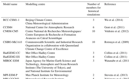
reference values have been obtained cover the period 1850– 2000 and are referred as historical in the fifth phase of the Coupled Model Intercomparison Project; (CMIP5, Taylor et al., 2012). The GCMs selected here (Table 1) are the ones for which the variables of interest for our diagnostics were available at the time of the analysis.
2.2 Data assimilation method
Table 1. CMIP5/PMIP3 GCMs characteristics and references.
Model name Modelling centre Number of Reference
members for historical simulations
BCC-CSM1-1 Beijing Climate Center, 3 Wu et al. (2014)
China Meteorological Administration
CCSM4 National Center for Atmospheric Research 6 Gent et al. (2011)
CNRM-CM5 Centre National de Recherches Meteorologiques/ 10 Voldoire et al. (2012)
Centre Europeen de Recherche et Formation Avancees en Calcul Scientifique
CSIRO-Mk3.6.0 Commonwealth Scientific and Industrial Research 10 Rotstayn et al. (2009)
Organization in collaboration with Queensland Climate Change Centre of Excellence
HadGEM2-CC Met Office Hadley Centre 3 Collins et al. (2011)
HadGEM2-ES Met Office Hadley Centre 4 Collins et al. (2011)
MIROC-ESM Japan Agency for Marine-Earth Science and 3 Watanabe et al. (2011)
Technology, Atmosphere and Ocean Research Institute (The University of Tokyo), and and National Institute for Environmental
MPI-ESM-P Max Planck Institute for Meteorology 2 Stevens et al. (2013)
MRI-CGCM3 Meteorological Research Institute 5 Yukimoto et al. (2012)
2009; Dubinkina et al., 2011), in a similar manner as in sev-eral recent studies (e.g. Goosse et al., 2012; Mathiot et al., 2013; Mairesse et al., 2013). First, an ensemble of 96 simu-lations (called particles) is initialized from a slightly different sea surface temperature for each particle, allowing different time developments. After one year of simulation, the like-lihood of each particle is computed from the difference be-tween the proxy-based reconstructed and the simulated sea ice concentration anomalies (6 ka minus PI results), taking into account the errors. Depending on their likelihood, i.e. their ability to reproduce the signal derived from the avail-able reconstructions, the particles are then either abandoned if their likelihood is low or kept as a basis for the next year’s simulation if their likelihood is high enough. In order to maintain a constant number of particles until the end of the simulated period, a resampling, depending on the particles likelihood, is conducted annually: the particles with a higher likelihood are copied more times than the others. Finally, the initial conditions of each particle are once more perturbed by adding a small noise to the sea surface temperature of the copies in order to obtain different time developments for the following year, and the whole procedure is repeated sequen-tially every year until the end of the simulation, here after 400 years.
2.3 Proxy-based sea ice reconstruction
The MH proxy-based sea ice reconstructions used to evalu-ate model performance and to constrain LOVECLIM sim-ulations is derived from cysts produced by dinoflagellates
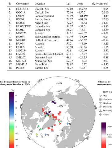
(dinocysts). The dinocyst distribution in Arctic and subarc-tic seas is indeed controlled by several environmental param-eters including productivity, salinity, temperature and, most importantly, sea ice (de Vernal and Rochon, 2011). The data set is based on the dinocyst content of 18 cores collected in the North Atlantic and Arctic oceans (Table 2 and Fig. 1). Sea ice is expressed in terms of annual mean concentration (in %) and is associated with a standard error of±11 % (de Vernal et al., 2013a). This value is used as the estimate of the recon-struction uncertainty for the evaluation of the likelihood in the experiment with data assimilation.
Table 2. Description of all the cores available at 6±0.5 ka (AD−4050±0.5 kyr) used to reconstruct sea ice cover (de Vernal et al., 2013a). The table shows the core ids used in this study, their name, location, latitude, longitude and the reconstructed sea ice concentration (sic ano) anomalies (reference period AD 1850–1900).
Id Core name Location Lat Long 6k sic ano (%)
1. HLY05JPC Chukchi Sea 72.69 −157.52 8.95
2. GGC19 Chukchi Sea 72.16 −155.51 22.60
3. LS009 Lancaster Sound 74.19 −81.195 −4.49
4. BS004 Barrow Strait 74.27 −91.09 12.60
5. HU008 Nares Strait 77.27 −74.32 −14.53
6. HU021TWC Labrador Sea 58.37 −57.51 −5.82
7. HU013 Labrador Sea 58.21 −48.31 −12.59
8. MD2227 Atlantic 58.21 −48.37 −5.08
9. HU044 East Canadian margin 44.49 −55.19 0.14
10. MD2033 Gulf of St Lawrence 44.66 −55.62 −0.52
11. HU094 Atlantic 50.2 −45.69 −8.25
12. HU085 Atlantic 53.98 −38.64 −1.85
13. MD2254 Atlantic 56.8 −30.66 3.53
14. HM025 Faroe–Shetland Channel 60.11 −6.07 1.61
15. JM1207 Denmark Strait 68.1 −29.35 0.88
16. M23323 Norwegian Sea 67.77 5.92 2.07
17. MSM712 Fram Strait 78.92 6.77 −5.45
18. PL112 Barents Sea 71.27 42.61 5.75
Figure 1. Reconstructions of sea ice conditions for the mid-Holocene. Diamonds markers with number next to them (refer to the left-hand coloured bar) correspond to MH sea ice concentration anomalies (in %) using the reference period AD 1850–1900 based on dinocyst assemblages (de Vernal et al., 2013a). The other markers with numbers inside are the MH sea ice signals derived from different sea ice proxies (see key on the right). Sea ice conditions are expressed in terms of more (blue) or less (red) sea ice in the MH as compared to a reference period which varies depending on the record but which generally covers most of the Holocene (see Table 3). The location of some proxies has been shifted slightly for an improved readability.
the accuracy is calculated from the residuals or difference between observed and estimated values and corresponds to the standard deviation of the residuals. In addition to the
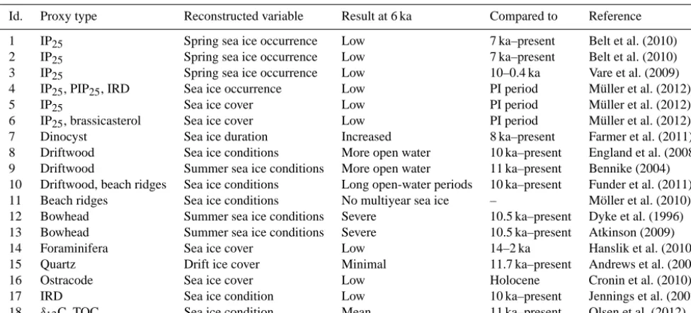
Table 3. Arctic sea ice reconstructions displayed in Fig. 1 and their signal in the MH as compared to the reconstruction means.
Id. Proxy type Reconstructed variable Result at 6 ka Compared to Reference
1 IP25 Spring sea ice occurrence Low 7 ka–present Belt et al. (2010)
2 IP25 Spring sea ice occurrence Low 7 ka–present Belt et al. (2010)
3 IP25 Spring sea ice occurrence Low 10–0.4 ka Vare et al. (2009)
4 IP25, PIP25, IRD Sea ice occurrence Low PI period Müller et al. (2012)
5 IP25 Sea ice cover Low PI period Müller et al. (2012)
6 IP25, brassicasterol Sea ice cover Low PI period Müller et al. (2012)
7 Dinocyst Sea ice duration Increased 8 ka–present Farmer et al. (2011)
8 Driftwood Sea ice conditions More open water 10 ka–present England et al. (2008)
9 Driftwood Summer sea ice conditions More open water 11 ka–present Bennike (2004)
10 Driftwood, beach ridges Sea ice conditions Long open-water periods 10 ka–present Funder et al. (2011)
11 Beach ridges Sea ice conditions No multiyear sea ice – Möller et al. (2010)
12 Bowhead Summer sea ice conditions Severe 10.5 ka–present Dyke et al. (1996)
13 Bowhead Summer sea ice conditions Severe 10.5 ka–present Atkinson (2009)
14 Foraminifera Sea ice cover Low 14–2 ka Hanslik et al. (2010)
15 Quartz Drift ice cover Minimal 11.7 ka–present Andrews et al. (2009)
16 Ostracode Sea ice cover Low Holocene Cronin et al. (2010)
17 IRD Sea ice condition Low 10 ka–present Jennings et al. (2002)
18 δ13C, TOC Sea ice condition Mean 11 ka–present Olsen et al. (2012)
indices of reliability have been proposed in order to assess the quality of reconstructions. In the present case, more than 95 % of reconstructions are labelled with high-quality indices (cf. de Vernal et al., 2013a, and data posted on the Geotop website).
The proxy records include variability on a (multi-)centennial timescale that could not be repro-duced in the time slice experiments performed following the PMIP protocol. Therefore, we consider the MH as a period of 1 kyr, i.e. 6±0.5 ka, which limits the contribution of internal variability and non-orbital forcings. The choice of such an interval length also allows us to neglect the potential biases related to dating uncertainties.
The model–data comparison and the data assimilation are performed using anomalies and considering the PI conditions (AD 1850–1900) as a reference period. We have preferred this option rather than using recent observed sea ice cover, since comparing sea ice conditions inferred from dinocyst content with satellite data would have led to additional un-certainties. Furthermore, the recent period is far from being adequate for calculating anomalies since it presents rapid changes characterized by a significant decrease in sea ice (e.g. Stroeve et al., 2011). Unfortunately, many of the avail-able reconstructed time series used here are not continuous up to AD 1900. We have thus decided to reconstruct the ref-erence data set by computing a linear interpolation of those time series up to the period AD 1850–1900. To avoid extrap-olating over too long periods, the proxy records ending be-fore 2 ka have been discarded from our analysis.
2.4 Experimental design
All the MH simulations represent equilibrium conditions cor-responding to 6 ka. They use the orbital forcing, following Berger (1978). The changes in greenhouse gas concentration are taken from Flückiger et al. (2002) for LOVECLIM simu-lations, which are slightly different from the ones used in the framework of the CMIP5/PMIP3 (http://pmip3.lsce.ipsl.fr/). As in Mathiot et al. (2013) and Mairesse et al. (2013), LOVE-CLIM simulations also consider slight changes in ice sheet topography and surface albedo, following the reconstruction of Peltier (2004), as well as in freshwater fluxes from Antarc-tic ice sheet melting according to the results of Pollard and DeConto (2009). This represents a small difference as com-pared to the CMIP5/PMIP3 protocol, as the latter prescribes present-day ice sheet topography and no change in freshwa-ter fluxes at 6 ka with respect to the present. However, this has virtually no effect on results.
For the reference period corresponding to the PI values, we have averaged all the results from available members for each GCM (Table 1) and from a set of experiments with LOVE-CLIM (Crespin et al., 2012) over the period AD 1850–1900 (over the period AD 1860–1900 in the cases of HadGEM2-CC and HadGEM2-ES).
3 Results and discussion
the quantitative proxy-based sea ice reconstructions based on dinocysts display heterogeneous and weak anomalies at 6 ka (Fig. 1). Lower annual mean sea ice concentration is recorded in the MH in the Fram Strait, northern Baffin Bay and Labrador Sea as compared to the PI period. By contrast, the MH is characterized by higher sea ice concentration in the Chukchi Sea, and to a lesser extent, in the Barents Sea and in the Barrow Strait (in the CAA; Fig. 1).
Overall, this data set appears consistent with other sea ice proxy-based reconstructions, even if the consistency can only be examined qualitatively since most of the available proxy-based sea ice reconstructions are qualitative or semi-quantitative. Furthermore, most of the mid-Holocene con-ditions depicted by those records are here compared to the whole (or most) of the Holocene and not to the PI period as displayed in our analysis, since data are often not valuable for the recent period. Information about these proxy records and their signal at 6 ka can be found in Table 3 and Fig. 1.
In the CAA, the MH sea ice record deduced from various proxies is very heterogeneous, which is consistent with the dinocyst-based records (id 3–5). On the one hand, the little amount of bowhead bones found indicates high sea ice cov-erage (Dyke et al., 1996; Atkinson, 2009), but, on the other hand, the analysis of IP25in several sediment cores suggests low spring sea ice occurrence in the MH compared to the whole Holocene period (Vare et al., 2009; Belt et al., 2010). This heterogeneity can, at least partly, be due to the numer-ous narrow straits being associated with different circulation patterns (e.g. Lietaer et al., 2008).
Further west, the higher sea ice concentration recorded over the Chukchi Sea in the MH (id 1 and 2) is in agreement with relatively low bottom-water temperature on the shelf as recorded from oxygen isotopes in benthic foraminifers (Farmer et al., 2011) as well as with the relatively low tem-perature shown by several proxies in Alaska (Kaufman et al., 2004).
The sea ice records show a relatively clear picture in the north of Greenland, Svalbard, the east of Greenland and in the Labrador Sea with globally less sea ice in the MH as compared to the Holocene period. Indeed, several sea ice condition reconstructions based on driftwood deposits and on beach ridges show rare or absent multiyear sea ice in the MH as far north as the northern coasts of Greenland (Bennike, 2004; Möller et al., 2010; Funder et al., 2011) and Ellesmere Island (England et al., 2008), while these coastlines are presently permanently surrounded by pack ice (Polyak et al., 2010). Note that according to (Olsen et al., 2012), northern Greenland displayed no strong signal in sea ice in the MH as compared to the whole Holocene, since this period was experiencing a shift in climate from warmer ditions associated with a reduced sea ice towards colder con-ditions and more prolonged winter ice cover. This MH shift is also recorded through the analysis of IP25in two sediment cores collected from the continental slope of West Spitsber-gen. They display lower sea ice cover in the MH as compared
to the end of the records covering the very late Holocene (Müller et al., 2012), consistent with the negative sea ice con-centration anomalies of core id 17.
Further south, along the East Greenland Shelf, the recon-struction of Müller et al. (2012) based on IP25and brassicast-erol and the reconstruction of Jennings et al. (2002) based on ice-rafted detritus are consistent and highlight relatively low sea ice cover in the MH as compared to the PI period and the whole Holocene period, respectively. The dinocyst-based re-construction from de Vernal et al. (2013a) adjacent from the previous reconstructions (id 15) shows no change at 6 ka as compared to the PI period.
Off northern Iceland, the extent of drift ice seemed to reach a minimum in the MH relative to the past 10 kyr, according to a reconstruction based on the presence of quartz (Andrews et al., 2009). Finally, since there is no other independent sea ice proxy-record, the positive sea ice concentration anoma-lies displayed in the Barents Sea (id 18) cannot be confirmed or rebutted.
The conclusions derived from the dinocyst-based recon-structions of de Vernal et al. (2013a) are thus generally qual-itatively confirmed by other proxy-based reconstructions, even if some discrepancies exist. However, out of the 18 proxy-based reconstructions, only four (id 2, 4, 5, and 7 on Fig. 1) have a larger signal than their error, i.e. does not have zero within the error bar. This has two implications for the following of this study to keep in mind. First, the potential of this data set to test the models’ performance is weak and, sec-ond, the constraint applied on the LOVECLIM results during the process of data assimilation will not be large.
3.2 Simulations without data assimilation
Here, the simulated sea ice signal in the MH on a large scale is first studied, before analysing the sea ice cover for the model grid points that contain the quantitative sea ice proxy record of de Vernal et al. (2013a) displayed in Fig. 1. We assume that the spatial representativeness of each core cor-responds to the matching grid cell of each model, while the latter have different spatial resolutions. We mainly focus on 8 of the 18 available cores (id 1–5, 15, 17 and 18) because the other ones are located south of the simulated sea ice edge for most of the GCMs and LOVECLIM for both the MH and the PI periods and thus display no change in sea ice concen-tration. Since the proxy records are calibrated to represent annual means, we primarily focus on the annual means of the models, although seasonal means are also considered in order to get a better understanding of the processes that drive the simulated sea ice cover.
Sea−ice concentration anomaly (%)
−60 −40 −20 0 20 40 60
(a)
Annual mean120
°
W
60
°
W
0°
60 ° E
120
° E
180
°
E
45° N 60° N
(b)
Winter (March)120
°
W
60
°
W
0°
60 ° E
120
° E
180
°
E
45° N 60° N
(c)
Summer (September)120
°
W
60
°
W
0°
60 ° E
120
° E
180
°
E
45° N 60° N
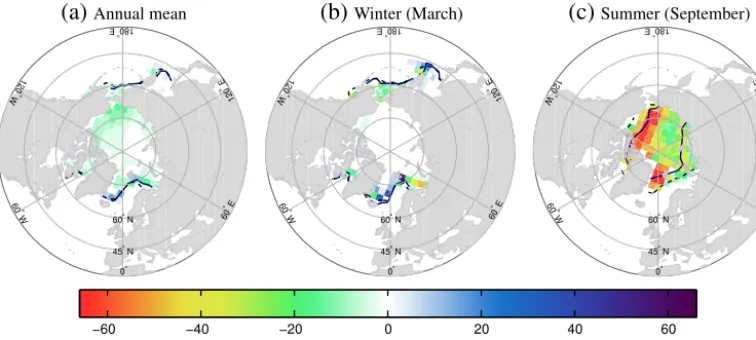
Figure 2. Mean annual, winter (March) and summer (September) MH sea ice concentration anomalies (in %, with respect to the PI reference period) and location of the ice edge for 6 ka (solid lines) and for the PI period (dashed lines), defined as 15 % concentration limits, as simulated by LOVECLIM without data assimilation.
hide larger differences in sea ice that occur in different sea-sons between the MH and the PI period. In winter, the sea ice tends to be more variable (Fig. 2b for LOVECLIM and Fig. A2), nearly all models simulating some regions with a higher ice extent and others with a sea ice retreat, but with different patterns. In summer, the agreement is better with a significantly decreased sea ice concentration in all the sectors (Fig. 2c for LOVECLIM and Fig. A3 for the other models).
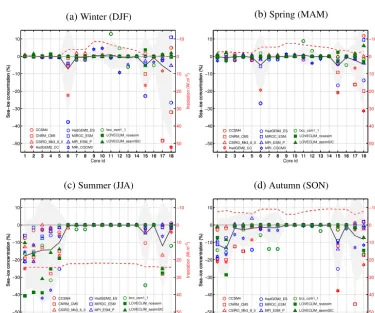
When looking at the locations of the sea ice reconstruc-tions, the simulated signal is homogeneous over the Chukchi Sea (id 1 and 2) and the CAA (id 3–5), where all models de-pict weak negative anomalies (Fig. 3). This annual decrease in sea ice cover is mainly due to a lower sea ice concentration in summer in response to the relatively strong increase in in-solation (on average 24 W m−2for these regions; Fig. 4c). To a lesser extent, fall also contributes to the decrease in annual sea ice cover especially in the Chukchi Sea, despite a dwin-dling insolation at 6 ka (on average −7 W m−2; Fig. 4d). This can be explained by the inertia of the system: higher summer insolation leads to a decrease in ice thickness and concentration in summer and thus larger oceanic heat fluxes during the following seasons (Manabe and Stouffer, 1980; Renssen et al., 2005; Boé et al., 2009; Crespin et al., 2012). No change in winter and spring sea ice cover is simulated over the Chukchi Sea and the CAA (Fig. 4a and b), these re-gions being then fully covered by sea ice and far from the ice edge (Fig. 2b for LOVECLIM and Fig. A2 for the other models).
In the Barents Sea (id 18), the annual mean sea ice concen-tration is also lower in the MH compared to the PI period for the majority of the models (Fig. 3). However, the spread is larger than in the Chukchi Sea and two GCMs (CCSM4 and MIROC-ESM) even display positive anomalies. These latter models show higher MH sea ice concentration all year long
with a maximum in spring which is consistent with the de-creased insolation during this season (−2.79 W m−2). As for the other models which show negative annual sea ice concen-tration anomalies, they have their maximum decrease in sea ice in fall (CSIRO-Mk3–6-0, MRI-CGCM3, BCC-CSM1– 1 and LOVECLIM; Fig. 4d) or in winter (CNRM-CM5, HadGEM2-CC, HadGEM2-ES and MPI-ESM-P; Fig. 4a). This contrasts with the previous situation since the maximum decrease in sea ice concentration appears delayed compared to the western Arctic and inconsistent with the insolation anomalies during the corresponding season (−7.92 W m−2 in fall and 0.04 W m−2in winter). However, this can easily be explained by the mean state of the models, i.e. the simu-lated sea ice concentration in absolute values for the PI pe-riod. In summer, the models cannot melt any sea ice in the MH compared to the PI since most of them depict almost ice-free conditions over the Barents Sea (Fig. 5). The models that have their maximum decrease in sea ice in fall are the ones that already display a reasonable ice cover during that season for the PI. The other models have a later beginning of the ice season (November–December) for the PI, and thus a maximum reduction at that time.
The annual mean simulated MH sea ice concentration is also lower in Fram Strait (id 17) and in the Greenland Sea (id 15) as compared to the PI values. As in the Barents Sea, the changes in insolation alone cannot explain the simulated sea ice cover fluctuations as they vary both in timing and in magnitude between the models. The simulated mean state likely plays a role there too but the interpretation seems more complex.
1 2 3 4 5 6 7 8 9 10 11 12 13 14 15 16 17 18 −30 −20 −10 0 10 20 Sea −
ice concentration (%)
Reconstructions CCSM4 CNRM−CM5 CSIRO−Mk3−6−0 HadGEM2−CC HadGEM2−ES MIROC−ESM MPI−ESM−P MRI−CGCM3 bcc−csm1−1 LOVECLIM−noassim
1 2 3 4 5 6 7 8 9 10 11 12 13 14 15 16 17 18
30 20 10 0 −10 −20 Insolation (W.m − 2)
1 2 3 4 5 6 7 8 9 10 11 12 13 14 15 16 17 18
−30 −20 −10 0 10 20 Core id Sea −
ice concentration (%)
Ch ukc hi S ea Ch ukc hi S ea sssdd dddd d
CAA Ch
ukc
hi Sea
sssdd
dddd
d
Fram
StraitChukchi S
ea
sssdd
dddd
d
Denmark StraitCh
ukc hi S ea sssdd dddd d Ba ren
ts SeaChukchi S
ea
sssdd
dddd
d LOVECLIM-assim-SIC
Figure 3. Mid-Holocene annual mean sea ice concentration anomalies (in %) for the proxy-based reconstructions of de Vernal et al. (2013a) (black diamonds with error bars) and the corresponding climate models results. The thick black line is the model mean. The grey shaded
areas are the model mean±2 standard deviations. The dashed red line represents the annual mean insolation at each location studied (in
W m−2) and corresponds to the reversed right axis. The reference period is AD 1850–1900.
(a)Winter (DJF)
Sea
−
ice concentration (%)
Core id
1 2 3 4 5 6 7 8 9 10 11 12 13 14 15 16 17 18
−50 −40 −30 −20 −10 0 10
1 2 3 4 5 6 7 8 9 10 11 12 13 14 15 16 17 18
50 40 30 20 10 0 −10 Insolation (W.m − 2) Sea −
ice concentration (%)
Core id
1 2 3 4 5 6 7 8 9 10 11 12 13 14 15 16 17 18
−50 −40 −30 −20 −10 0 10 CNRM_CM5 CSIRO_Mk3_6_0 HadGEM2_CC HadGEM2_ES MIROC_ESM MPI_ESM_P MRI_CGCM3 bcc_csm1_1 LOVECLIM_noassim LOVECLIM_assimSIC CCSM4
(b)Spring (MAM)
Core id
Sea
−
ice concentration (%)
1 2 3 4 5 6 7 8 9 10 11 12 13 14 15 16 17 18
−50 −40 −30 −20 −10 0 10 CCSM4 CNRM_CM5 CSIRO_Mk3_6_0 HadGEM2_CC HadGEM2_ES MIROC_ESM MPI_ESM_P MRI_CGCM3 bcc_csm1_1 LOVECLIM_noassim LOVECLIM_assimSIC
1 2 3 4 5 6 7 8 9 10 11 12 13 14 15 16 17 18
50 40 30 20 10 0 −10 Insolation (W.m − 2) Core id Sea −
ice concentration (%)
1 2 3 4 5 6 7 8 9 10 11 12 13 14 15 16 17 18
−50 −40 −30 −20 −10 0 10
(c)Summer (JJA)
Sea
−
ice concentration (%)
Core id
1 2 3 4 5 6 7 8 9 10 11 12 13 14 15 16 17 18
−50 −40 −30 −20 −10 0 10
1 2 3 4 5 6 7 8 9 10 11 12 13 14 15 16 17 18
50 40 30 20 10 0 −10 Insolation (W.m − 2) Sea −
ice concentration (%)
Core id
1 2 3 4 5 6 7 8 9 10 11 12 13 14 15 16 17 18
−50 −40 −30 −20 −10 0 10 CNRM_CM5 CSIRO_Mk3_6_0 HadGEM2_CC HadGEM2_ES MIROC_ESM MPI_ESM_P MRI_CGCM3 bcc_csm1_1 LOVECLIM_noassim LOVECLIM_assimSIC CCSM4
(d)Autumn (SON)
Sea
−
ice concentration (%)
Core id
1 2 3 4 5 6 7 8 9 10 11 12 13 14 15 16 17 18
−50 −40 −30 −20 −10 0 10
1 2 3 4 5 6 7 8 9 10 11 12 13 14 15 16 17 18
50 40 30 20 10 0 −10 Insolation (W.m − 2) Sea −
ice concentration (%)
Core id
1 2 3 4 5 6 7 8 9 10 11 12 13 14 15 16 17 18
−50 −40 −30 −20 −10 0 10 CCSM4 CNRM_CM5 CSIRO_Mk3_6_0 HadGEM2_CC HadGEM2_ES MIROC_ESM MPI_ESM_P MRI_CGCM3 bcc_csm1_1 LOVECLIM_noassim LOVECLIM_assimSIC
Figure 4. Mid-Holocene seasonal mean sea ice concentration anomalies (in %) for the climate model results corresponding to the core
locations. The thick black line corresponds to the model mean. The grey shaded areas are the model mean±2 standard deviations. The
dashed red line represents the seasonal mean insolation at each studied location (in W m−2) and corresponds to the reversed right axis. The
(a)Mid-Holocene
J F M A M J J A S O N D 0
10 20 30 40 50 60 70 80 90 100
Time of the year
Sea
−
ice concentration (%)
CCSM4 CNRM_CM5 CSIRO_Mk3_6_0 HadGEM2_CC HadGEM2_ES MIROC_ESM MPI_ESM_P MRI_CGCM3 bcc_csm1_1 LOVECLIM_noassim LOVECLIM_assimSIC
(b)Pre-industrial
J F M A M J J A S O N D 0
10 20 30 40 50 60 70 80 90 100
Sea
−
ice concentration (%)
Time of the year
Figure 5. Mid-Holocene (6 ka) and pre-industrial (AD 1850–1900) mean seasonal cycles of sea ice concentration (in %) in the Barents Sea (at the location of the proxy-based reconstruction id 18).
proxy data; red lines on Fig. 6) and spatially more homo-geneous (the average of standard deviations equals 4.5 % compared to 8.8 %). The most noticeable discrepancy be-tween models and data occurs in the Chukchi Sea, where all models simulate a lower sea ice concentration while the two proxy-based reconstructions show the opposite (Fig. 3). This could be partly due to the misrepresentation of the exchanges between the Arctic and the Pacific through the Bering Strait by the models. The very heterogeneous sea ice cover recorded over the CAA is also not reproduced by the models, but this was expected given that the com-plex circulation pattern has local effects on sea ice (e.g. Lietaer et al., 2008). In the Fram Strait, the sea ice record agrees with the model mean signal. This is not the case in the Denmark Strait and in the Barents Sea where the mean simulated sea ice anomalies are negative while the proxy-based reconstructions show positive anomalies (Fig. 3), even if some models are able to reproduce the sign and magnitude of the reconstructed signal.
A more quantitative way to study the (dis)agreement be-tween models and data is to compute the root mean square error (RMSE) between the results of each climate model and the proxy-based sea ice reconstructions (Fig. 6). The val-ues range from 9 to 14 %. The models are in better agree-ment amongst themselves than with the proxy-based recon-structions since the difference in RMSE between any of the models is smaller (largest difference is equal 5 %) than any RMSE using the reconstruction. Furthermore, assuming no change in sea ice concentration between the MH and the PI period provides an even lower RMSE than any of the mod-els (this is equivalent to computing the RMSE using a con-stant field of anomalies being equal to zero; see the purple bar on Fig. 6). However, those RMSE should be analysed with caution. First, the calculation is performed based on the difference between each proxy-based reconstruction and the simulated sea ice in the corresponding grid cell. This means
0 1 2 3 4 5 6 7 8 9 10 11 12 13 14 15
Models
RMSE (%)
CNRM
−CM5
HadGEM2 −CC
LC−
noassim
HadGEM2 −ES
bcc−
csm1 −1
MRI
−CGCM3
MPI
−ESM
−P
LC−
assim SIC
CSIRO
−Mk3
−6 −0
MIROC
−ESMCCSM4
Anomalies=0 LOVECLIM without data assimilation LOVECLIM with data assimilation No change between MH and PI
Sea-ice con
centratio
n (%)
Figure 6. Ranked RMSE between the MH sea ice anomalies (ref-erence period AD 1850–1900) simulated by each model and the proxy-based reconstructions. The error bars correspond to the range of the RMSE when changing the reference period to AD 1850–1875 and AD 1875–1900. The purple bar is the RMSE computed assum-ing no change between the MH and the PI and is thus a measure of the mean signal of the data. The dashed red line is the estimate of the mean data error (to be read with the right axis). The red lines are the mean signals of the models and the data (purple bar), both esti-mated as the mean of the absolute value of the difference between the MH and the PI period (to be read with the right axis).
to the non-climatic noise present in the proxies and in the uncertainties in the reconstruction method, or to the biases of models results. This prevents estimating explicitly the mod-els’ skills as done, for instance, in Hargreaves et al. (2013) and in Mairesse et al. (2013) for temperature data. The main robust conclusion is that models and reconstructions agree that the changes between the MH and the PI period annual mean sea ice concentration are relatively weak.
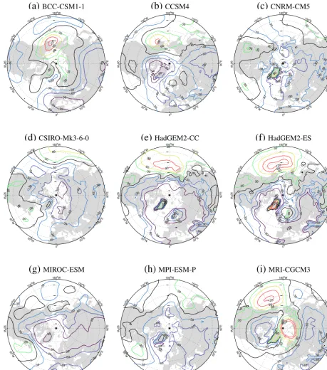
On a larger scale, the atmospheric circulation changes may explain the spatial structure of the simulated sea ice anoma-lies in various models. Here, the atmospheric circulation is inferred from the surface pressure of the GCMs because the geopotential heights were not available for all of them at the time of the analysis. For the LOVECLIM simulations, we preferred using the geopotential heights at the pressure level 800 hPa because it is a direct dynamical variable that gives more reliable results than the surface pressure. We have checked the models for which both the geopotential heights and the surface pressure were available and, qualitatively, these two variables give the same atmospheric patterns.
The simulated atmospheric circulation changes between the MH and the PI are relatively weak, and appear to have a relatively complex spatial structure (Figs. 7 and 8). Over-all, the models disagree on many aspects of the changes, although some common atmospheric patterns can be found in spring (a trend similar to a more negative Arctic Os-cillation regime), summer and autumn (higher geopotential height over the northern Pacific and globally lower over the Eurasian continent) (not shown). Depending on the model selected, the atmospheric circulation can initially exacerbate or mitigate the decreased sea ice cover due to the higher summer insolation over the Chukchi Sea. Indeed, some mod-els display atmospheric circulation patterns that tend to in-duce some sea ice convergence towards that region (e.g. CCSM4, MRI-CGCM3, MIROC-ESM) or to push it away (e.g. LOVECLIM no assim, BCC-CSM1-1). Nevertheless, the link between atmospheric circulation and sea ice concen-tration is hard to estimate because of the likely dominant role of the thermodynamical response to insolation changes.
The role of the atmospheric circulation does not appear to be clearer in the Barents Sea, where the positive annual anomalies displayed by CCSM4 and MIROC-ESM cannot be explained by the respectively southerly and easterly wind anomalies simulated there, although the northerly winds sim-ulated by CNRM-CM5 could explain the large negative sea ice anomalies simulated by this model. The different re-sponses of the models appear thus to imply too many pro-cesses to be analysed in the present framework using avail-able diagnostics. The potential role of atmospheric circula-tion will be more deeply analysed in the next seccircula-tion, involv-ing data assimilation. In that particular case, model physics is the same and the only differences are the ones induced by the data constraint, which manifests itself in our experiments mainly through atmospheric circulation changes.
3.3 Simulations with data assimilation
Without assimilation, the sea ice concentration simulated by LOVECLIM shows some clear differences with the best esti-mates given by the reconstructions of de Vernal et al. (2013a) (Fig. 6), especially in the Chukchi Sea where the model dis-plays the most negative anomalies among all models while the proxy-based reconstructions show positive ones (Fig. 3). As expected, data assimilation leads to better agreement with the majority of the proxy-based reconstructions (compare the green triangles in Fig. 3 with the green squares). In particular over the Chukchi Sea (id 1 and 2), LOVECLIM with data as-similation has an annual mean ice concentration higher than LOVECLIM without data assimilation, respectively 9.7 and 12.1 % where cores 1 and 2 are located. This strong increase is, however, not sufficient to get positive anomalies, since over that region, the increase of the simulated sea ice can only occur in summer and autumn, the rest of the year be-ing already fully covered by sea ice in the MH. However, the significantly higher insolation in summer and its lingering effect in autumn prevents any massive increase in sea ice. Furthermore, the proxy-based reconstruction uncertainty is larger than the signal depicted by the first core, which leads to a constraint too weak to get positive anomalies.
Over the CAA (id 3–5), the signal of the proxy-based re-constructions is too heterogeneous to be simulated by LOVE-CLIM. Compared to the simulation without data assimila-tion, the simulation with data assimilation provides a slightly increased annual mean sea ice concentration because of a less reduced summer sea ice. Yet the annual anomalies are still negative, which is consistent with two out of the three cores located there (id 3 and 5). In the Denmark Strait (id 15), the consistency between LOVECLIM and the proxy-based reconstruction is lower after data assimilation, due to a de-creased winter and spring sea ice concentration (Fig. 4a and b). However, the simulated sea ice stays within the range of the proxy-based reconstruction error.
(a)
BCC-CSM1-1 150 oW 120 oW 90 o W 60 o W 30o W 0o 30 oE 60 oE 90 oE 120 o E 150o E 180o W 30 30 30 30 60 90 120 −90 −90 −90 −90 −60 −60 −60 −30 −30 −30 −30 −30 0 0 0 0(b)
CCSM4 150 oW 120 oW 90 o W 60 o W 30o W 0o 30 oE 60 oE 90 oE 120 o E 150o E 180o W 30 30 60 90 −90 −90 −60 −60 −60 −60 −60 −60 −60 −30 −30 −30 −30 −30 −30 −30 0 0 0 0 0 0 0 0(c)
CNRM-CM5 150 oW 120 oW 90 o W 60 o W 30o W 0o 30 oE 60 oE 90 oE 120 o E 150o E 180o W 30 30 30 30 30 30 60 −90 −60 −60 −60 −60 −60 −60 −30 −30 −30 −30 −30 −30 −30 −30 −30 −30 −30 −30 −30 −30 −30 −30 −30 −30 0 0 0 0 0 0 0 0(d)
CSIRO-Mk3-6-0 150 oW 120 oW 90 o W 60 o W 30o W 0o 30 oE 60 oE 90 oE 120 o E 150 o E 180o W 30 30 30 30 60 −90 −90 −60 −60 −60 −60 −60 −30 −30 −30 −30 −30 −30 −30 −30 −30 −30 −30 0 0 0 0 0(e)
HadGEM2-CC 150 oW 120 oW 90 o W 60 o W 30o W 0o 30 oE 60 oE 90 oE 120 o E 150 o E 180o W 30 30 30 30 60 90 90 −90 −90 −90 −90 −90 −60 −60 −60 −60 −60 −60 −30 −30 −30 −30 −30 −30 −30 −30 −30 −30 0 0 0 0 0 0 0 0 0(f)
HadGEM2-ES 150 oW 120 oW 90 o W 60 o W 30o W 0o 30 oE 60 oE 90 oE 120 o E 150 o E 180o W 30 30 30 30 30 30 30 60 60 90 90 120 120 −90 −90 −90 −90 −90 −90 −60 −60 −60 −60 −60 −60 −30 −30 −30 −30 −30 −30 −30 −30 −30 0 0 0 0 0 0 0 0 0 0 0(g)
MIROC-ESM 150 oW 120 oW 90 o W 60 o W 30o W 0o 30 oE 60 oE 90 oE 120 o E 150 o E 180o W 30 −90 −90 −90 −90 −60 −60 −60 −60 −60 −30 −30 −30 −30 −30 −30 0 0 0 0 0(h)
MPI-ESM-P 150 oW 120 oW 90 o W 60 o W 30o W 0o 30 oE 60 oE 90 oE 120 o E 150 o E 180o W 30 30 −90 −90 −60 −60 −60 −60 −60 −60 −60 −30 −30 −30 −30 −30 −30 0 0 0 0 0(i)
MRI-CGCM3 150 oW 120 oW 90 o W 60 o W 30o W 0o 30 oE 60 oE 90 oE 120 o E 150 o E 180o W 30 30 30 30 60 60 60 90 90 120 120 −60 −60 −60 −60 −30 −30 −30 −30 −30 −30 −30 −30 −30 −30 −30 −30 0 0 0 0 0 0 0 0Figure 7. Annual mean surface pressure anomalies (in Pa) simulated by the GCMs for the MH (reference period AD 1850–1900).
in the RMSE of the model (not shown). This core is thus not critical to the assimilation process on a large scale, LOVE-CLIM being able to fit the new core values locally without significantly altering the sea ice results somewhere else.
Overall, the data assimilation leads to a modest decrease of the RMSE (9.6 % compared to 12.8 %; Fig. 6), but the agreement between LOVECLIM with data assimilation and
(a)Without data assimilation
150 oW
120
oW
90
o
W
60o W
30oW
0o
30oE 60oE
90
oE 120
o E 150oE 180oW
−10 −8
−8
−8
−6 −6
−6
−4
−4 −4
−4
−2 −2
−2
−2
0 0
0
2
2
4 6 8 8
10
0 0
0
(b)With data assimilation
150 oW
120
oW
90
o
W
60o W
30oW
0o
30oE 60oE
90
oE 120
o E 150oE 180oW
−8 −8
−6 −6
−4 −4
−4 −4
−2 −2
−2
0 0
2
2 4
4 4 6
6
8
0 0
0
Figure 8. MH annual geopotential height anomalies (in m) at 800 hPa simulated by (a) LOVECLIM without assimilation and (b) LOVECLIM with assimilation of sea ice proxy data. The reference period is AD 1850–1900.
150
oW
120
oW
90
o
W
60 o W
30oW
0o
30oE
60
oE
90
oE 120
o E 150o
E 180oW
−−54−3
−3
−2
−2
−1
−1
−1 0
0
0 0
1
1 1
2 2
2
2
3 3 4 5
0
0
0 0
Figure 9. Difference between the geopotential height anomalies (in m) at 800 hPa of LOVECLIM with sea ice data assimilation and LOVECLIM without data assimilation. The black arrows show the flow responsible for the change in sea ice at the Barents Sea and the Chukchi Sea.
data. Consequently, the potential to significantly modify the way LOVECLIM simulates the sea ice for the MH is limited. Furthermore, the spatial resolution is rather coarse in LOVE-CLIM and, therefore, it cannot take into account small spatial scale processes potentially dominant over regional processes for some records.
The improved consistency between the simulation with sea ice data assimilation and the sea ice proxy-based reconstruc-tions is associated mainly with higher sea ice concentration in the Chukchi Sea and in the Barents Sea. This is achieved through changes in the atmospheric circulation. Indeed, the
higher pressure anomaly centred on the Aleutians in the sim-ulation with data assimilation compared to the simsim-ulation without data assimilation leads to a cooling in the Chukchi Sea and to a convergence of sea ice in that region (Fig. 9). On the other side of the Arctic, the lower pressure anomaly centred on Russia is responsible for a cooling over the Bar-ents Sea and thus leads to the increased simulated sea ice where core 18 is located.
4 Conclusions
We have compared new quantitative reconstructions of mean annual sea ice concentration in the MH with models output. Overall, the sea ice changes between the MH and the PI pe-riod are relatively weak both in the simulations and the re-constructions but they are weaker and spatially more homo-geneous in models. The simulated ice changes are higher for individual seasons, with a relatively strong sea ice retreat in summer and a more variable sea ice during winter. This un-derlines the need for quantitative seasonal reconstructions for a more comprehensive model–data comparison in the future. A general agreement between models and proxy-based re-constructions is found in the Labrador Sea while a large dis-crepancy occurs in the Chukchi Sea, where models are not able to reproduce the relatively high sea ice concentration reconstructed for the MH compared to the PI period. How-ever, the uncertainty of the reconstructions, which is of the same order as the changes, prevents a precise evaluation of the models’ skills on a regional scale.
Greenland and the Barents Sea, the simulated sea ice con-centration is more variable amongst models meaning that the agreement between models and data depends on the model considered. Over the whole Arctic, but particularly in these regions, the mean state of the models influences the timing of the simulated sea ice changes with a reduction of the MH sea ice concentration compared to PI values obviously only at the time when there is already sea ice in the PI. In addition to the role of insolation and to the link between the mean state and the model response, it is difficult in the present framework to precisely identify the mechanisms that control the simulated sea ice concentration for all models.
Appendix A
Sea−ice concentration anomaly (%)
−60 −40 −20 0 20 40 60
(a)
BCC-CSM1-1120
°
W
60
°
W
0°
60 ° E
120
° E
180
°
E
45° N 60° N
(b)
CCSM4120
°
W
60
°
W
0°
60 ° E
120
° E
180
°
E
45° N 60° N
(c)
CNRM-CM5120
°
W
60
°
W
0°
60 ° E
120
° E
180
°
E
45° N 60° N
(d)
CSIRO-Mk3-6-0120
°
W
60
°
W
0°
60 ° E
120
° E
180
°
E
45° N 60° N
(e)
HadGEM2-CC120
°
W
60
°
W
0°
60 ° E
120
° E
180
°
E
45° N 60° N
(f)
HadGEM2-ES120
°
W
60
°
W
0°
60 ° E
120
° E
180
°
E
45° N 60° N
(g)
MIROC-ESM120
°
W
60
°
W
0°
60 ° E
120
° E
180
°
E
45° N 60° N
(h)
MPI-ESM-P120
°
W
60
°
W
0°
60 ° E
120
° E
180
°
E
45° N 60° N
(i)
MRI-CGCM3120
°
W
60
°
W
0°
60 ° E
120
° E
180
°
E
45° N 60° N
Acknowledgements. We thank the editor and two anonymous reviewers for valuable suggestions during the review process which improved the final version of this paper. We acknowledge all those involved in producing the PMIP an CMIP multi-model ensemble and all the climate modelling groups for making available their model output. We acknowledge the World Climate Research Programme’s Working Group on Coupled Modelling, which is responsible for CMIP. For CMIP the US Department of Energy’s Program for Climate Model Diagnosis and Intercomparison provides coordinating support and led development of software infrastructure in partnership with the Global Organization for Earth System Science Portals. The research leading to these results has received funding from the European Union’s Seventh Framework programme (FP7/2007–2013) under grant agreement no. 243908, “Past4Future: Climate change – Learning from the past climate”. Computational resources have been provided by the supercomputing facilities of the Université catholique de Louvain (CISM/UCL) and the Consortium des Equipements de Calcul Intensif en Fédération Wallonie Bruxelles (CECI) funded by FRS-FNRS. Hugues Goosse is senior research associate with the FRS/FNRS, Belgium. This is Past4Future contribution 66.
Edited by: V. Rath
References
Andrews, J. T., Darby, D., Eberle, D., Jennings, A. E., Moros, M., and Ogilvie, A.: A robust, multisite Holocene history of drift ice off northern Iceland: implications for North Atlantic climate, The Holocene, 19, 71–77, doi:10.1177/0959683608098953, 2009. Atkinson, N.: A 10 400-Year-Old Bowhead Whale (Balaena
mys-ticetus) Skull from Ellef Ringnes Island, Nunavut: Implications for Sea-Ice Conditions in High Arctic Canada at the End of the Last Glaciation, Arctic, 62, 38–44, 2009.
Belt, S. T., Vare, L. L., Massé, G., Manners, H. R., Price, J. C., MacLachlan, S. E., Andrews, J. T., and Schmidt, S.: Strik-ing similarities in temporal changes to sprStrik-ing sea ice occur-rence across the central Canadian Arctic Archipelago over the last 7000 years, Quaternary Sci. Rev., 29, 3489–3504, doi:10.1016/j.quascirev.2010.06.041, 2010.
Bennike, O.: Holocene sea-ice variations in
Green-land: onshore evidence, The Holocene, 14, 607–613,
doi:10.1191/0959683604hl722rr, 2004.
Berger, A.: Long-term variations of daily insolation and Quaternary climatic changes, J. Atmos. Sci., 35, 2363–2367, 1978. Berger, M., Brandefelt, J., and Nilsson, J.: The sensitivity of
the Arctic sea ice to orbitally induced insolation changes: a study of the mid-Holocene Paleoclimate Modelling Intercom-parison Project 2 and 3 simulations, Clim. Past, 9, 969–982, doi:10.5194/cp-9-969-2013, 2013.
Boé, J., Hall, A., and Qu, X.: Current GCMs’ Unrealistic Neg-ative Feedback in the Arctic, J. Climate, 22, 4682–4695, doi:10.1175/2009JCLI2885.1, 2009.
Braconnot, P., Otto-Bliesner, B., Harrison, S., Joussaume, S., Pe-terchmitt, J.-Y., Abe-Ouchi, A., Crucifix, M., Driesschaert, E., Fichefet, Th., Hewitt, C. D., Kageyama, M., Kitoh, A., Laîné, A., Loutre, M.-F., Marti, O., Merkel, U., Ramstein, G., Valdes, P., Weber, S. L., Yu, Y., and Zhao, Y.: Results of PMIP2 coupled simulations of the Mid-Holocene and Last Glacial Maximum –
Part 1: experiments and large-scale features, Clim. Past, 3, 261– 277, doi:10.5194/cp-3-261-2007, 2007.
Braconnot, P., Harrison, S. P., Kageyama, M., Bartlein,
P. J., Masson-Delmotte, V., Abe-Ouchi, A., Otto-Bliesner, B., and Zhao, Y.: Evaluation of climate models using palaeoclimatic data, Nature Climate Change, 2, 417–424, doi:10.1038/nclimate1456, 2012.
Brovkin, V., Bendtsen, J., Claussen, M., Ganopolski, A., Kubatzki, C., Petoukhov, V., and An-dreev, A.: Carbon cycle, vegeta-tion, and climate dynamics in the Holocene: Experiments with the CLIMBER-2 model, Global Biogeochem. Cy., 16, 1139, doi:10.1029/2001GB001662.1., 2002.
Collins, W. J., Bellouin, N., Doutriaux-Boucher, M., Gedney, N., Halloran, P., Hinton, T., Hughes, J., Jones, C. D., Joshi, M., Lid-dicoat, S., Martin, G., O’Connor, F., Rae, J., Senior, C., Sitch, S., Totterdell, I., Wiltshire, A., and Woodward, S.: Develop-ment and evaluation of an Earth-System model – HadGEM2, Geosci. Model Dev., 4, 1051–1075, doi:10.5194/gmd-4-1051-2011, 2011.
Crespin, E., Goosse, H., Fichefet, T., Mairesse, A., and Sallaz-Damaz, Y.: Arctic climate over the past millennium: Annual and seasonal responses to external forcings, The Holocene, 23, 321– 329, doi:10.1177/0959683612463095, 2012.
Cronin, T., Gemery, L., Briggs, W., Jakobsson, M., Polyak, L., and Brouwers, E.: Quaternary Sea-ice history in the Arctic Ocean based on a new Ostracode sea-ice proxy, Quaternary Sci. Rev., 29, 3415–3429, doi:10.1016/j.quascirev.2010.05.024, 2010. de Vernal, A. and Rochon, A.: Dinocysts as tracers of sea-surface
conditions and sea-ice cover in polar and subpolar environments, IOP Conference Series: Earth and Environmental Science, 14, 012007, doi:10.1088/1755-1315/14/1/012007, 2011.
de Vernal, A., Hillaire-Marcel, C., Rochon, A., Fréchette, B., Henry, M., Solignac, S., and Bonnet, S.: Dinocyst-based recon-structions of sea ice cover concentration during the Holocene in the Arctic Ocean, the northern North Atlantic Ocean and its adjacent seas, Quaternary Sci. Rev., 79, 111–121, doi:10.1016/j.quascirev.2013.07.006, 2013a.
de Vernal, A., Rochon, A., Fréchette, B., Henry, M., Radi, T., and Solignac, S.: Reconstructing past sea ice cover of the Northern Hemisphere from dinocyst assemblages: sta-tus of the approach, Quaternary Sci. Rev., 79, 122–134, doi:10.1016/j.quascirev.2013.06.022, 2013b.
Dubinkina, S., Goosse, H., Sallaz-Damaz, Y., Crespin, E., and Cru-cifix, M.: Testing a particle filter to reconstruct climate changes over past centuries, Int. J. Bifurcat. Chaos, 21, 3611–3618, doi:10.1142/S0218127411030763, 2011.
Dyke, A. S., Hooper, J., and Savelle, J. M.: A History of Sea Ice in the Canadian Arctic Archipelago Based on Postglacial Remains of the Bowhead Whale (Balaena mysticetus), Arctic, 49, 235– 255, 1996.
Ebert, E. E. and Curry, J. A.: An intermediate one-dimensional
thermodynamic sea ice model for investigating
ice-atmosphere interactions, J. Geophys. Res., 98, 10085–10109, doi:10.1029/93JC00656, 1993.
Farmer, J. R., Cronin, T. M., de Vernal, A., Dwyer, G. S., Keig-win, L. D., and Thunell, R. C.: Western Arctic Ocean tempera-ture variability during the last 8000 years, Geophys. Res. Lett., 38, L24602, doi:10.1029/2011GL049714, 2011.
Flückiger, J., Monnin, E., Stauffer, B., Schwander, J., and Stocker,
T. F.: High-resolution Holocene N2O ice core record and its
re-lationship with CH4and CO2, Global Biogeochem. Cy., 16,
10-1–10-8, 2002.
Francis, J. and Vavrus, S. J.: Evidence linking Arctic amplifica-tion to extreme weather in mid-latitudes, Geophys. Res. Lett., 39, L06801, doi:10.1029/2012GL051000, 2012.
Funder, S., Goosse, H., Jepsen, H., Kaas, E., Kjæ r, K. H., Ko-rsgaard, N. J., Larsen, N. K., Linderson, H., Lyså, A., Möller, P., Olsen, J., and Willerslev, E.: A 10,000-year record of Arc-tic Ocean sea-ice variability-view from the beach, Science, 333, 747–50, doi:10.1126/science.1202760, 2011.
Gent, P. R., Danabasoglu, G., Donner, L. J., Holland, M. M., Hunke, E. C., Jayne, S. R., Lawrence, D. M., Neale, R. B., Rasch, P. J., Vertenstein, M., Worley, P. H., Yang, Z.-L., and Zhang, M.: The Community Climate System Model Version 4, J. Climate, 24, 4973–4991, doi:10.1175/2011JCLI4083.1, 2011.
Goosse, H. and Fichefet, T.: Importance of ice-ocean interactions for the global ocean circulation: A model study, J. Geophys. Res., 104, 23337–23355, 1999.
Goosse, H., Brovkin, V., Fichefet, T., Haarsma, R., Huybrechts, P., Jongma, J., Mouchet, A., Selten, F., Barriat, P.-Y., Campin, J.-M., Deleersnijder, E., Driesschaert, E., Goelzer, H., Janssens, I., Loutre, M.-F., Morales Maqueda, M. A., Opsteegh, T., Mathieu, P.-P., Munhoven, G., Pettersson, E. J., Renssen, H., Roche, D. M., Schaeffer, M., Tartinville, B., Timmermann, A., and Weber, S. L.: Description of the Earth system model of intermediate complex-ity LOVECLIM version 1.2, Geosci. Model Dev., 3, 603–633, doi:10.5194/gmd-3-603-2010, 2010.
Goosse, H., Crespin, E., Dubinkina, S., Loutre, M.-F., Mann, M. E., Renssen, H., Sallaz-Damaz, Y., and Shindell, D.: The role of forcing and internal dynamics in explaining the ”Me-dieval Climate Anomaly”, Clim. Dynam., 39, 2847–2866, doi:10.1007/s00382-012-1297-0, 2012.
Goosse, H., Roche, D., Mairesse, A., and Berger, M.: Mod-elling past sea ice changes, Quaternary Sci. Rev., 79, 191–206, doi:10.1016/j.quascirev.2013.03.011, 2013.
Hanslik, D., Jakobsson, M., Backman, J., Björck, S., Sel-lén, E., O’Regan, M., Fornaciari, E., and Skog, G.: Quater-nary Arctic Ocean sea ice variations and radiocarbon reser-voir age corrections, Quaternary Sci. Rev., 29, 3430–3441, doi:10.1016/j.quascirev.2010.06.011, 2010.
Hargreaves, J. C., Annan, J. D., Ohgaito, R., Paul, A., and Abe-Ouchi, A.: Skill and reliability of climate model ensembles at the Last Glacial Maximum and mid-Holocene, Clim. Past, 9, 811– 823, doi:10.5194/cp-9-811-2013, 2013.
Holland, M. M. and Bitz, C. M.: Polar amplification of cli-mate change in coupled models, Clim. Dynam., 21, 221–232, doi:10.1007/s00382-003-0332-6, 2003.
Jennings, A. E., Knudsen, K. L., Hald, M., Hansen, C. V., and Andrews, J. T.: A mid-Holocene shift in Arctic sea-ice vari-ability on the East Greenland Shelf, The Holocene, 12, 49–58, doi:10.1191/0959683602hl519rp, 2002.
Kaufman, D., Ager, T., Anderson, N., Andersond, P., Andrews, J., Bartlein, P., Brubaker, L., Coats, L., Cwynar, L., Duvall, M.,
Dyke, A., Edwards, M., Eisner, W., Gajewski, K., Geirsdottir, A., Kaplan, M., Kerwin, M., Lozhkin, A., MacDonald, G., Miller, G., Mock, C., Oswald, W., Otto-Bliesner, B., Porinchu, D., Ruh-land, K., Smol, J., Steig, E., and Wolfe, B.: Holocene thermal
maximum in the western Arctic (0–180◦W), Quaternary Sci.
Rev., 23, 529–560, doi:10.1016/j.quascirev.2003.09.007, 2004. Lietaer, O., Fichefet, T., and Legat, V.: The effects of resolving the
Canadian Arctic Archipelago in a finite element sea ice model, Ocean Model., 24, 140–152, doi:10.1016/j.ocemod.2008.06.002, 2008.
Lohmann, G. and Gerdes, R.: Sea Ice Effects on the Sensitivity of the Thermohaline Circulation*, J. Climate, 11, 2789–2803, doi:10.1175/1520-0442(1998)011<2789:SIEOTS>2.0.CO;2, 1998.
Mairesse, A., Goosse, H., Mathiot, P., Wanner, H., and Dubink-ina, S.: Investigating the consistency between proxy-based re-constructions and climate models using data assimilation: a mid-Holocene case study, Clim. Past, 9, 2741–2757, doi:10.5194/cp-9-2741-2013, 2013.
Manabe, S. and Stouffer, R. J.: Sensitivity of a Global Climate Model to an Increase of CO2 Concentration in the Atmosphere, J. Geophys. Res., 85, 5529–5554, doi:10.1029/JC085iC10p05529, 1980.
Massonnet, F., Fichefet, T., Goosse, H., Bitz, C. M., Philippon-Berthier, G., Holland, M. M., and Barriat, P.-Y.: Constraining projections of summer Arctic sea ice, The Cryosphere, 6, 1383– 1394, doi:10.5194/tc-6-1383-2012, 2012.
Mathiot, P., Goosse, H., Crosta, X., Stenni, B., Braida, M., Renssen, H., Van Meerbeeck, C. J., Masson-Delmotte, V., Mairesse, A., and Dubinkina, S.: Using data assimilation to investigate the causes of Southern Hemisphere high latitude cooling from 10 to 8 ka BP, Clim. Past, 9, 887–901, doi:10.5194/cp-9-887-2013, 2013.
Möller, P., Larsen, N. K., Kjaer, K. H., Funder, S., Schomacker, A., Linge, H., and Fabel, D.: Early to middle Holocene valley glaciations on northernmost Greenland, Quaternary Sci. Rev., 29, 3379–3398, doi:10.1016/j.quascirev.2010.06.044, 2010. Müller, J., Werner, K., Stein, R., Fahl, K., Moros, M., and
Jansen, E.: Holocene cooling culminates in sea ice os-cillations in Fram Strait, Quaternary Sci. Rev., 47, 1–14, doi:10.1016/j.quascirev.2012.04.024, 2012.
Notz, D. and Marotzke, J.: Observations reveal external driver for Arctic sea-ice retreat, Geophys. Res. Lett., 39, 1–6, doi:10.1029/2012GL051094, 2012.
Olsen, J., Kjaer, K. H., Funder, S., Larsen, N. K., and Ludikova, A.: High-Arctic climate conditions for the last 7000 years inferred from multi-proxy analysis of the Bliss Lake record, North Green-land, J. Quaternary Sci., 27, 318–327, doi:10.1002/jqs.1548, 2012.
Opsteegh, B. J. D., Haarsma, R. J., Selten, F. M., Kattenberg, A., and Bilt, D.: ECBILT : a dynamic alternative to mixed boundary conditions in ocean models, Tellus A, 50, 348–367, 1998. Otto-Bliesner, B. L., Joussaume, S., Braconnot, P., Harrison, S. P.,
and Abe-Ouchi, A.: Modeling and Data Syntheses of Past Cli-mates: Paleoclimate Modelling Intercomparison Project Phase II Workshop, EOS T. Am. Geophys. Un., 90, 2009.
Peltier, W.: Global glacial isostasy and the surface of
GRACE, Annu. Rev. Earth and Pl. Sc., 32, 111–149, doi:10.1146/annurev.earth.32.082503.144359, 2004.
Pollard, D. and DeConto, R. M.: Modelling West Antarctic ice sheet growth and collapse through the past five million years, Nature, 458, 329–32, doi:10.1038/nature07809, 2009.
Polyak, L., Alley, R. B., Andrews, J. T., Brigham-Grette, J., Cronin, T. M., Darby, D. A., Dyke, A. S., Fitzpatrick, J. J., Funder, S., Holland, M., Jennings, A. E., Miller, G. H., O’Regan, M., Savelle, J., Serreze, M., St. John, K., White, J. W., and Wolff, E.: History of sea ice in the Arctic, Quaternary Sci. Rev., 29, 1757– 1778, doi:10.1016/j.quascirev.2010.02.010, 2010.
Renssen, H., Goosse, H., Fichefet, T., Brovkin, V., Driesschaert, E., and Wolk, F.: Simulating the Holocene climate evolu-tion at northern high latitudes using a coupled atmosphere-sea ice-ocean-vegetation model, Clim. Dynam., 24, 23–43, doi:10.1007/s00382-004-0485-y, 2005.
Renssen, H., Seppä, H., Heiri, O., Roche, D. M., Goosse, H., and Fichefet, T.: The spatial and temporal complexity of the Holocene thermal maximum, Nat. Geosci., 2, 411–414, doi:10.1038/ngeo513, 2009.
Rotstayn, L. D., Collier, M. A., Dix, M. R., Feng, Y., Gordon, H. B., O’Farrell, S. P., Smith, I. N., and Syktus, J.: Improved simulation of Australian climate and ENSO-related rainfall variability in a global climate model with an interactive aerosol treatment, Int. J. Climatol., 30, 1067–1088, doi:10.1002/joc.1952, 2009. Screen, J. A. and Simmonds, I.: The central role of diminishing
sea ice in recent Arctic temperature amplification, Nature, 464, 1334–7, doi:10.1038/nature09051, 2010.
Serreze, M. C., Holland, M. M., and Stroeve, J.: Perspectives on the Arctic’s shrinking sea-ice cover, Science, 315, 1533–1536, doi:10.1126/science.1139426, 2007.
Serreze, M. C., Barrett, A. P., Stroeve, J. C., Kindig, D. N., and Hol-land, M. M.: The emergence of surface-based Arctic amplifica-tion, The Cryosphere, 3, 11–19, doi:10.5194/tc-3-11-2009, 2009. Stevens, B., Giorgetta, M., Esch, M., Mauritsen, T., Crueger, T., Rast, S., Salzmann, M., Schmidt, H., Bader, J., Block, K., Brokopf, R., Fast, I., Kinne, S., Kornblueh, L., Lohmann, U., Pincus, R., Reichler, T., and Roeckner, E.: The atmospheric component of the MPI-M earth system model: ECHAM6, Journal of Advances in Modeling Earth Systems, 5, 1–27, doi:10.1002/jame.20015, 2013.
Stroeve, J. C., Serreze, M. C., Holland, M. M., Kay, J. E., Malanik, J., and Barrett, A. P.: The Arctic’s rapidly shrinking sea ice cover: a research synthesis, Climatic Change, 110, 1005–1027, doi:10.1007/s10584-011-0101-1, 2011.
Stroeve, J. C., Kattsov, V., Barrett, A., Serreze, M., Pavlova, T., Hol-land, M., and Meier, W. N.: Trends in Arctic sea ice extent from CMIP5, CMIP3 and observations, Geophys. Res. Lett., 39, 1–7, doi:10.1029/2012GL052676, 2012.
Sundqvist, H. S., Zhang, Q., Moberg, A., Holmgren, K., Körnich, H., Nilsson, J., and Brattström, G.: Climate change between the mid and late Holocene in northern high latitudes – Part 1: Survey of temperature and precipitation proxy data, Clim. Past, 6, 591– 608, doi:10.5194/cp-6-591-2010, 2010.
Taylor, K. E., Stouffer, R. J., and Meehl, G. A.: An Overview of CMIP5 and the Experiment Design, B. Am. Meteorol. Soc., 93, 485–498, doi:10.1175/BAMS-D-11-00094.1, 2012.
van Leeuwen, P. J.: Particle Filtering in Geophysical Systems, Mon. Weather Rev., 137, 4089–4114, doi:10.1175/2009MWR2835.1, 2009.
Vare, L. L., Massé, G., Gregory, T. R., Smart, C. W., and Belt, S. T.: Sea ice variations in the central Canadian Arctic Archipelago during the Holocene, Quaternary Sci. Rev., 28, 1354–1366, doi:10.1016/j.quascirev.2009.01.013, 2009.
Voldoire, A., Sanchez-Gomez, E., Salas y Mélia, D., Decharme, B., Cassou, C., Sénési, S., Valcke, S., Beau, I., Alias, A., Cheval-lier, M., Déqué, M., Deshayes, J., Douville, H., Fernandez, E., Madec, G., Maisonnave, E., Moine, M.-P., Planton, S., Saint-Martin, D., Szopa, S., Tyteca, S., Alkama, R., Belamari, S., Braun, A., Coquart, L., and Chauvin, F.: The CNRM-CM5.1 global climate model: description and basic evaluation, Clim. Dynam., 40, 2091–2121, doi:10.1007/s00382-011-1259-y, 2012. Wanner, H., Beer, J., Bütikofer, J., Crowley, T. J., Cubasch, U., Flückiger, J., Goosse, H., Grosjean, M., Joos, F., Kaplan, J. O., Küttel, M., Müller, S. A., Prentice, I. C., Solomina, O., Stocker, T. F., Tarasov, P., Wagner, M., and Widmann, M.: Mid- to Late Holocene climate change: an overview, Quaternary Sci. Rev., 27, 1791–1828, doi:10.1016/j.quascirev.2008.06.013, 2008. Watanabe, S., Hajima, T., Sudo, K., Nagashima, T., Takemura, T.,
Okajima, H., Nozawa, T., Kawase, H., Abe, M., Yokohata, T., Ise, T., Sato, H., Kato, E., Takata, K., Emori, S., and Kawamiya, M.: MIROC-ESM 2010: model description and basic results of CMIP5-20c3m experiments, Geosci. Model Dev., 4, 845–872, doi:10.5194/gmd-4-845-2011, 2011.
Wu, T., Song, L., Li, W., Wang, Z., Zhang, H., Xin, X., Zhang, Y., Zhang, L., Li, J., Wu, F., Liu, Y., Zhang, F., Shi, X., Chu, M., Zhang, J., Fang, Y., Wang, F., Lu, Y., Liu, X., Wei, M., Liu, Q., Zhou, W., Dong, M., Zhao, Q., Ji, J., Li, L., and Zhou, M.: An overview of BCC climate system model development and ap-plication for climate change studies, Journal of Meteorological Research, 28, 34–56, doi:10.1007/s13351-014-3041-7, 2014. Yukimoto, S., Adachi, Y., Hosaka, M., Sakami, T., Yoshimura, H.,
Hirabara, M., Tanaka, T. Y., Shindo, E., Tsujino, H., Deushi, M., Mizuta, R., Yabu, S., Obata, A., Nakano, H., Koshiro, T., Ose, T., and Kitoh, A.: A New Global Climate Model of the Meteo-rological Research Institute: MRI-CGCM3 – Model Description and Basic Performance –, J. Meteorol. Soc. Jpn., 90A, 23–64, doi:10.2151/jmsj.2012-A02, 2012.