Comparison between HDL simulation and MATLAB For Image Compression



COMPARISON

BETWEEN

HDL

SIMULATION

AND

MATLAB

FOR

IMAGE

COMPRESSION

Shailenndra Chouhan, Shweta Karnik

Department of Electronics and Communication

Shiv Kumar Singh Institute of Technology and Science, Indore, (M.P.)

ABSTRACT- THE DISCRETE WAVELET TRANSFORM (DWT) TECHNIQUE COMMONLY USED FOR DATA AND IMAGE

COMPRESSION. THIS PAPER SHOWN AN APPROACH FOR THE

COMPARISON BETWEEN HDL SIMULATION AND MATLAB TOOL

WHICH ARE USED IN THE IMAGE COMPRESSION FIELD. DWT

ALGORITHM IS DESIGNED IN HDL SIMULATION WHICH IS

VERILOG HDL LANGUAGE USING THE FILTER METHOD FOR THE

IMAGE COMPRESSION.DAUBECHIES (DB2)TAP FILTER IS USED IN

THIS DESIGN AND THE COEFFICIENTS OF DAUBECHIES FILTERS

FOR THE DWT TECHNIQUE ARE FIXED. RESULTS OF HDL

SIMULATION AND MATLAB TOOL ARE COMPARED AND IT IS

FOUND THAT THE INTENSITY OF THE COMPRESSED IMAGE USING

MATLAB TOOL IS HIGHER THAN THAT OF HDL SIMULATION. Index Terms- Wavelet Transform, Fourier Transform, Dwt (Discrete Wavelet Transform), Daubechies (Db2) Wavelet Filter

I. INTRODUCTION

Data compression is the technique to reduce the redundancies in data representation in order to decrease data storage requirements and hence communication costs. Reducing the storage requirement is equivalent to increasing the capacity of the storage medium and hence communication bandwidth. Thus the development of efficient compression techniques will continue to be a design challenge for future communication systems and advanced multimedia applications.

Data is represented as a combination of information and redundancy. Information is the portion of data that must be preserved permanently in its original form in order to correctly interpret the meaning or purpose of the data. Redundancy is that portion of data that can be removed when it is not needed or can be reinserted to interpret the data when needed. Most often, the redundancy is reinserted in order to generate the original data in its original form. A technique to reduce the redundancy of data is defined as Data compression. The redundancy in data representation is reduced such a way that it can be subsequently reinserted to recover the original data, which is called decompression of the data.

Applications of data compression are primarily in transmission and storage of information. Image transmission applications are in broadcast television, remote sensing via

satellite, military communication via aircraft, radar and sonar, teleconferencing, and computer communications.

II. WAVELET TRANSFORM

The transform of a signal is just another form of representing the signal. It does not change the information content present in the signal. The Wavelet Transform provides a time-frequency representation of the signal. It was developed to overcome the short coming of the Short Time Fourier Transform (STFT), which can also be used to analyze non-stationary signals. While STFT gives a constant resolution at all frequencies, the Wavelet Transform uses multi-resolution technique by which different frequencies are analyzed with different resolutions.

The wavelet analysis is done similar to the STFT analysis. The signal to be analyzed is multiplied with a wavelet function just as it is multiplied with a window function in STFT, and then the transform is computed for each segment generated. However, unlike STFT, in Wavelet Transform, the width of the wavelet function changes with each spectral component. The Wavelet Transform, at high frequencies gives good time resolution and poor frequency resolution, while at low frequencies the Wavelet Transform gives good frequency resolution and poor time resolution.

III. DWT AND FILTER BANKS

The Wavelet Series is just a sampled version of CWT and its computation may consume significant amount of time and resources, depending on the resolution required. The Discrete Wavelet Transform (DWT), which is based on sub-band coding, is found to yield a fast computation of Wavelet Transform. It is easy to implement and reduces the computation time and resources required.

In CWT, the signals are analyzed using a set of basis functions which relate to each other by simple scaling and translation. In the case of DWT, a time-scale representation of the digital signal is obtained using digital filtering techniques. The signal to be analyzed is passed through filters with different cutoff frequencies at different scales.

determined by the filtering operations, and the scale is determined by up sampling and down sampling (sub sampling) operations.

The DWT is computed by successive low pass and high pass filtering of the discrete time-domain signal. This is called the Mallat algorithm or Mallat-tree decomposition. Its significance is in the manner it connects the continuous time mutiresolution to discrete-time filters. In the figure, the signal is denoted by the sequence x[n], where n is an integer. The low pass filter is denoted by g[n] while the high pass filter is denoted by h[n]. At each level, the high pass filter produces detail information, while the low pass filter associated with scaling function produces coarse approximations.

The reconstructions of the original signal from the wavelet coefficients. Basically, the reconstruction is the reverse process of decomposition. The approximation and detail coefficients at every level are up sampled by two, passed through the low pass and high pass synthesis filters and then added. This process is continued through the same number of levels as in the decomposition process to obtain the original signal.

A. One level of the transform

The DWT of a signal x is calculated by passing it through a series of filters. First the samples are passed through a low pass filter with impulse response g resulting in a convolution of the two:

The signal is also decomposed simultaneously using a high-pass filter h. The output giving the details of coefficients (from the high-pass filter) and approximation coefficients (from the low-pass). It is important that the two filters are related to each other and they are known as a quadrature mirror filter. However, since half the frequencies of the signal have now been removed, half the samples can be discarded according to Nyquist’s rule. The filter outputs are then sub sampled by 2 (Mallat's and the common notation is the opposite, g- high pass and h- low pass)

Fig.1. One level of transform

B. Multi-Resolution Analysis using Filter Banks

Filters are one of the most widely used signal processing functions. Wavelets can be realized by iteration of filters

determined by up sampling and down sampling (sub sampling) operations.

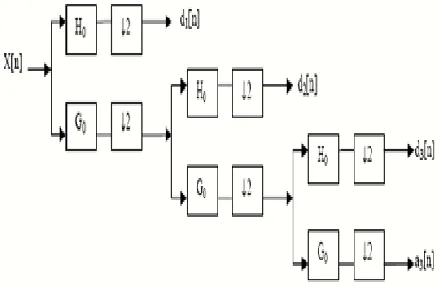
The DWT is computed by successive low pass and high pass filtering of the discrete time-domain signal as shown in figure 02. This is called the Mallat algorithm or Mallat-tree decomposition. Its significance is in the manner it connects the continuous time mutiresolution to discrete-time filters. In the figure, the signal is denoted by the sequence x[n], where n is an integer. The low pass filter is denoted by G0 while the high pass filter is denoted by H0. At each level, the high pass filter produces detail information; d[n], while the low pass filter associated with scaling function produces coarse approximations, a[n].

Fig.2. Three-level wavelet decomposition trees

IV. DISCRETE WAVELET TRANSFORM OPERATION

When a signal passes through these filters, it is split into two bands. The low pass filter, which corresponds to an averaging operation, extracts the coarse information of the signal. The high pass filter, which corresponds to a differencing operation, extracts the detail information of the signal. The output of the filtering operations is then decimated by two.

two-dimensional transform (see Figure 03) can be accomplished by performing two separate one-dimensional transforms. First, the image is filtered along the x dimension and decimated by two. Then, it is followed by filtering the sub-image along the y-dimension and decimated by two. Finally, we have split the image into four bands denoted by LL, HL, LH and HH after one-level decomposition.

of the energy in each of these three sub bands is concentrated in the vicinity of areas corresponding to edge activities in the original image. Since LL1 is a coarser approximation of the input, it has similar spatial and statistical characteristics to the original image. As a result, it can be further decomposed into four sub bands LL2, LH2, HL2 and HH2 as shown in figure 03 based on the principle of Multiresolution analysis. Accordingly the image is decomposed into any number of levels. The same computation can continue to further decompose LL2 into higher levels.

Fig. 3. Extension of DWT in two - dimensional signals

V. IMPLEMENTATION OF DWTALGORITHM

The DWT Algorithm is implemented using Verilog HDL on Altera’s Quartus II 9.0 Web Edition tool.

In DWT module it consists of low pass, high pass filter and a down sampler module. Low pass filter, high pass filter and down sample are coded in different module. After designing these modules a top level module is designed using low pass, high pass and down sample module to DWT. This top level module is the DWT module. The pixel value of the image is taken as a input of the DWT algorithm and this input is processed by low pass and high pass filter followed by a down sampler. The output of the high pass filter is wavelet coefficients and the output of the low pass filter is the scaling coefficients. Now in second stage the outputs of the low pass filter become the inputs for the second stage of DWT algorithm. In a similar way further DWT scaling and wavelet coefficients are computed.

VI. RTL OF DWTALGORITHM

clk clk_enable reset filter_in[63..0] filter_out[63..0] clk clk_enable reset filter_in[63..0] filter_out[63..0] clk clk_enable reset sample_gin[63..0] sample_fin[63..0] clk_2 sample_gout[63..0] clk clk_enable reset filter_in[63..0] filter_out[63..0] clk clk_enable reset filter_in[63..0] filter_out[63..0] clk clk_enable reset sample_gin[63..0] sample_fin[63..0] clk_2 sample_gout[63..0] clk clk_enable reset filter_in[63..0] filter_out[63..0] clk clk_enable reset filter_in[63..0] filter_out[63..0] clk clk_enable reset sample_gin[63..0] sample_fin[63..0] sample_gout[63..0] hp:hiD1 lp:loD1 downsample1:downs1 hp:hiD2 lp:loD2 downsample1:downs2 g[63..0] g_g[63..0] g_g_g[63..0] reset2 filter_in[63..0] reset clk_enable clk reset1 lp:loD downsample:downs hp:hiD

Fig. 4. RTL of DWT Algorithm

VII. RESULTS

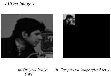
The grayscale cameraman image of 64x64 pixels is taken as an input (generated with the help of MATLAB Tool) for the DWT algorithm designed in HDL and is compressed at two levels. After two level compressions, the image is represented by 16x16 pixels. The compressed simulated data is in binary format thus to visualize these compressed data image plotting tool of MATLAB is used. Figure 04 and figure 05 shows the original image and compressed image using HDL simulation and MATLAB tool. The compressed image is basically the LL-2 part of the DWT algorithm. DWT algorithm for image compression can be used at any level of compression.

The DWT algorithm is designed and verified with the help of simulation. This algorithm is designed in verilog HDL so it can be implemented on the hardware. This DWT algorithm gives the compressed result of input image. This result is verified with the help of simulation tool.

A. Compression using HDL Simulation

1)

(a) Original Image (b) Compressed Image after 2 level

B. Compression using MATLAB Tool

1)

(a) Original Image (b) Compressed Image after 2 level

DWT

Fig. 5.Compression using HDL and MATLAB Tool

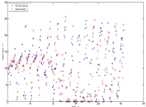
C. Comparison between HDL Simulation and Matlab Results

The Graph isplotted using MATLAB tool and results of HDL simulation and MATLAB tool can be analyzed with the help of graph.

Fig. 5.Graph between HDL and MATLAB simulation Result for Test Image 1

D. Compression using HDL Simulation

1)

(a) Original Image (b) Compressed Image after 2 level

E. Compression using MATLAB Tool

1)

(a) Original Image (b) Compressed Image after 2 level

DWT

Fig. 6.Compression using HDL and MATLAB Tool

F. Comparison between HDL Simulation and Matlab Results

The Graph isplotted using MATLAB tool and results of HDL simulation and MATLAB tool can be analyzed with the help of graph.

Fig. 7.Graph between HDL and MATLAB simulation Result for Test Image 1

VIII. CONCLUSION

using HDL. The number of DWT stages can be varied, resulting in different number of sub bands. Different filter banks with different characteristics can be used. Efficient fast algorithm (pyramidal computing scheme) for the computation of discrete wavelet coefficients makes a wavelet transform based encoder computationally efficient.

REFERENCES

[1] Abdullah AlMuhit, Md. Shabiul Islam and Masuri Othman, VLSI Implementation of Discrete Wavelet Transform (DWT) for Image

Compression, 2nd International Conference on Autonomous Robots

and Agents December 13-15, 2004 Palmerston North, New Zealand

on VLSI.

[2] Sonja Grgic, Kresimir Kers, Mislav Grgic, Image Compression using

Wavelets Bled Slovenia ISIE, 1999. Chen, Linear Networks and

Systems (Book style). Belmont, CA: Wadsworth, 1993,

[3] Martin Vetterli, Wavelets and Fiter Banks: Theory and Design, IEEE transaction on signal Processing, Vol. 40,No. 9, September 1992. [4] Ibrahim Oz Cemil Oz Nejat Yumusak, Image Compression using 2-D

Multi-Level Discrete Wavelet Transform (DWT).

[5] R.C. Gonzalez and R. E. Woods, Digital Image Processing, Reading. MA Addison Wesley, 2004.

[6] David Salomon, Data Compression, The Complete Reference, 2nd Edition Springer-Verlag 1998.

[7] http://en.wikipedia.org/wiki/Discrete_wavelet_transform on 15 May 2012.

[8] Chris Solomon and Toby Breckon, Fundamentals of Digital Image Processing A Practical Approach with Examples in Matlab.

[9] http://users.minet.uni-jena.de/~sack/SS04/download/IEEE-754.html on 12 April 2012.