A Practical Approach Deriving Optimal Unit Hydrograph from Noisy Runoff in absence of Rainfall Data

(1)

Article

1

A Practical Approach Deriving Optimal Unit

2

Hydrograph from Noisy Runoff in absence of

3

Rainfall Data

4

Kee-Won Seong 1,*

5

1_{Department of Civil Engineering, College of Engineering, Konkuk University, 120 Neungdong-ro,}

6

Gwangjin-gu, Seoul 05029, Korea; [email protected]

7

* Correspondence: [email protected]; Tel: +82-2-450-3450

8

Abstract: As a procedure deriving UH (unit hydrograph), the root selection method necessitates

9

only storm runoff data. However, this method must deal with the uncertainty related to the noise

10

fluctuation of runoff ordinates and derive one optimal UH from many storms. This study proposes

11

a procedure that applies the Savitzky-Golay filter to smooth the noise fluctuation of the runoff

12

ordinates and uses the linear combination of UHs from individual storms to derive an optimal UH.

13

The proposed method is applied to the storms of the Nenagh River basin in Ireland. The

14

applicability of the Savitzky-Golay filter for smoothing the noise fluctuation of storm runoffs is

15

examined by means of the Nash-Sutcliffe efficiency index. Furthermore, the root selection method

16

is extended to also estimate IUHs. The results show that the adoption of the Savitzky-Golay filter

17

improves the applicability of the root selection method and that the optimal UH predicts accurately

18

the time-to-peak and peak discharge.

19

Keywords: root selection method; unit hydrograph; Savitzky-Golay filter; Nash-Sutcliffe index

20

21

1. Introduction

22

The unit hydrograph (UH) concept is generally used for the analysis of rainfall-runoff

23

relationship since it is practically convenient to describe linearly the basin response to rainfall input.

24

Numerous methods have been proposed to find an UH from storm hydrographs with known

25

rainfall inputs. However, one still needs an efficient method estimating the UH in absence of rainfall

26

input. For unknown rainfall input in hydrograph analysis, several researches focused on separating

27

a UH from the runoff hydrograph. De Laine [1] suggested the root matching method using the roots

28

of the polynomial representing the Z-transform of a hydrograph of finite length. Turner et al. [2]

29

proposed an alternative approach that is less sensitive to data quality than that of De Laine [1]. This

30

approach called the root selection method used the Argand diagram to decide the shape of a

31

resulting UH. Based on Turner et al. [2], Ojha et al. [3] applied scaling parameters to adjust the

32

values of UH coordinates. To improve UH determination, Parmentier et al. [4] proposed a method

33

that avoids the subjective selection of rainfall roots by identifying and controlling the

34

time-dependent response components. Bruen et al. [5] extended the applicability of the root selection

35

method in separating urbanization effects in runoff data. Based on the theory of response separation

36

provided by the root selection method, Seong [6] suggested a novel method estimating the

37

parameters of the Clark’s IUH.

38

Though the root selection method has shown satisfactory results in determining a UH, the

39

uncertainties in UH ordinates and the derivation of a representative UH based on multiple storm

40

events remain still matters to be considered. De Laine [1] and Turner et al. [7] showed that the root

41

selection method produces remarkably sensitive roots for the polynomial representing a single

42

storm runoff hydrograph. This means that the uncertainties polluting the runoff hydrographs from

43

different storms will affect sensitively each UH polynomial for the corresponding storm. To reduce

44

such uncertainties, this study applies the five-point Savitzky-Golay filter to runoff data [8,9]. By

45

(2)

applying the filter, the variation of UH ordinates extracted from different storms can be diminished

46

within a narrow range so that the important UH parameters such as peak value and time-to-peak

47

exhibit more stable values.

48

Even though the smoothing filter is applied, a UH based on individual storm event usually

49

differs from one storm to another. Occasionally, the estimate of UH from a single event will yield

50

unreliable result showing unsatisfactory value of goodness-of-fit index. Thus, this research suggests

51

a method by which an optimum UH is derived from available multiple storm events. To do this, this

52

research combines the UH polynomials from multiple storm events based on the linear combination

53

theory. In addition, this research investigates the applicability of IUHs obtained from UHs resulting

54

from the root selection by comparing them with existing IUHs obtained from a conventional

55

method.

56

The validity of the proposed methodology is verified using the 22 storm records of the Nenagh

57

River at Claianna, Ireland, which are adopted in the referred researches concerning the root selection

58

method and investigating other general rainfall-runoff relationships [2,3,7,10,11].

59

2. Method

60

2.1 Smoothing of Runoff Data by the Savitzky-Golay Filter

61

Though runoff data can be collected by a proper way, there is still an uncertainty associated

62

with natural randomness that might affect the root selection procedure. The uncertainty of runoff

63

data appears frequently in the form of oscillations in the hydrograph. If rainfall data is available for

64

rainfall-runoff analysis, this uncertainty can be eliminated or reduced by minimizing error

65

techniques such as the least squares method or other regression methods. Moreover, the concurrent

66

use of multiple storms in the convolution procedure would lower the uncertainties when deriving

67

UH. However, in absence of rainfall data, the root selection method cannot consider the uncertainty

68

of runoff data and will result in relatively higher variation of the UH ordinates obtained from

69

different storms. In signal processing field, these oscillations from randomness are generally

70

eliminated by data smoothing. Among the various smoothing techniques, the Savitzky-Golay filter

71

is adopted in this research since it tends to preserve the peak heights of a given noisy signal. Such

72

characteristics of the Savitzky-Golay filter makes it particularly adapted for deriving UH, especially

73

when associated with the root selection method.

74

For a runoff data y=

{

q1, , qn

}

consisting of n discharge ordinates, the Savitzky-Golay filter

75

fits a polynomial of arbitrary order to the2m+1data points surrounding the center for data

76

smoothing. Chau [9] proposed the following expression involving a set of weights wj for this

77

polynomial:

78

* 1

2 1

m

i j i j

j m

q w q

m =− +

=

+



, (1)

where q*i denote the smoothed discharge ordinates and qi j+ are the original runoff ordinates, in

79

which i and j are the running indices. It is known that the Savitzky-Golay filter uses the least-squares

80

technique to find the weights wj. For example, the best quadratic polynomial smoothing data to the

81

surrounding five data values (m = 2 for 2m+1 = 5) is expressed in Equation (2):

82

(

)

*

2 1 1 2

1

3 12 17 12 3

35

i i i i i i

q = − q₋ + q₋ + q + q₊ − q₊ . (2)

This study adopts Equation (2) to smooth the runoff because it involves the lesser number of runoff

83

data points in the smoothing process. Equation (2) requires the first and last points to be treated.

84

Here, an artificial extension of data by adding zeros is employed.

85

2.2 The Root Selection Method

(3)

The linear discrete convolution relationship between a pulse response function being UH, an

87

input being effective rainfall and an output being runoff is usually expressed as Equation (3) [6]:

88

(

)

(

)

0

( ) n ( )

i

y nT h iT x n i T

=



− , (3)

where T is the time interval for sampling; the output y nT( ) is the runoff sampled at t nT= ; and,

89

the input x n

(

−1

)

T

)

is the effective rainfall between times t= −

(

n 1

)

T and nT . The pulse

90

response function h iT( ) represents the ordinate value of T-period UH at time t=iT i, =0n. As

91

for Equation (3), De Laine [1] proposed the root matching method to estimate the UH without using

92

rainfall data. The root matching method uses the Z-transformation method for rainfall-runoff

93

modelling in frequency domain. Thus, Equation (3) can be rewritten as:

94

1 1 1

( ) ( ) ( )

Y z− =H z− X z− , (4)

where Y z( −1) is a polynomial resulting from the Z-transform of direct runoff y; X z( −1) is a

95

polynomial representing the Z-transform of rainfall x; and, H z( −1) is a polynomial indicating the

96

Z-transform of UH. The root matching method uses the roots of the runoff polynomial Y z( −1) to

97

give H z( −1). According to De Laine [1], from the results of multiple runoff analysis, the common

98

roots in more than two runoff polynomials can be extracted because the common roots are

99

independent of the rainfall and thus, the UH can be constructed using these common roots.

100

However, Turner et al. [2] showed that the root matching method is sensitive to the errors in runoff

101

data and proposed a new method finding the UH polynomial by considering the roots on the

102

complex plot (or the Argand diagram) of the runoff polynomial. Based on the analysis using

103

synthetic data and real runoff data, they found a specific feature of the roots reflecting UH on the

104

Argand diagram. Furthermore, the authors showed that this feature was practically common to all

105

runoff events in a same basin. Finally, Turner et al. [2] suggested a procedure (the root selection

106

method) that could extract UH roots from the runoff roots on the Argand diagram and showed that

107

the method gave a smaller average error in UH than the root matching method.

108

2.3 Determination of an Optimal UH for Multiple Storm Events

109

The root selection method has been successful in identifying UH roots from a runoff

110

polynomial based on individual single runoff event. However, a practical procedure is still

111

necessary to determine the optimal UH obtained from multiple runoff events. Accordingly, this

112

study constructs an optimal runoff polynomial by selecting the optimal UH roots from a unique and

113

integrated Argand diagram in which all runoff roots appear. The suggested method involves the

114

following processes:

115

1 smoothening of fluctuation in ordinates of runoff hydrographs by the Savitzky-Golay filter

116

based on large number of runoff data;

117

2 selection of the UH roots for each storm runoff data by conventional root selection procedure,

118

and derivation of the individual single-event UH polynomial;

119

3 overlapping of the UH roots selected individually from different storm runoffs on the Argand

120

diagram from one storm to another;

121

4 removal of eventual abnormal roots based on thick circular pattern that might indicate the

122

uncertainty associated with natural randomness of runoff process;

123

5 reconstruction of the UH polynomial for each storm by considering the removed roots in step 4,

124

and normalization of each coefficient of the polynomial by dividing each coefficient by the sum

125

of all coefficients;

126

7 construction of an optimal UH polynomial by linear combination of the UH polynomials for

127

storms considered to be a response to one unit of the effective rainfall for a specified duration

128

(4)

The above-mentioned procedure can be formulated mathematically as follows. Consider k storm

130

runoffs y y=

[

1, ,ym, ,yk

]

 _ _

in which ym represents the direct runoff data for the mth storm

131

event. Each ordinate of ym becomes one coefficient of the runoff polynomial when applying the

132

Z-transform to runoff y_m. The same notation applies for the UHs h=

[

h₁, , h_m, , h_k

]

and for the

133

effective rainfall series x x=

[

1, ,xm, ,xk

]

 _ _

using the relationship given in Equation (3). Equation

134

(4) is also generalized by introducing a subscript denoting the event number. The resulting

135

convolution equation replacing Equation (4) is then:

136

1 1 1

( ) ( ) ( ), 1, ,

m m m

Y z− =H z− X z− m=  k. (5)

Since this work uses the smoothed runoff obtained by the Savitzky-Golay filter instead of the raw

137

runoff data Y zm( −1), Equation (5) is rewritten with the smoothed runoff Y zm*( −1) as shown in

138

Equation (6):

139

*₍ 1₎ ₍ 1₎ ₍ 1_), _{1, ,}

m m m

Y z− =H z− X z− m=  k, (6)

where Ym*(z−1)=Z y

( )

*m ; and, y*m represents the smoothed runoff data for the mth storm.

140

Considering UH polynomials for k storms H zm( −1) with m=1, , k, the coefficients of H zm( −1)

141

do not indicate the ordinates of UH for storm number k but represent simply the relative values

142

between the coefficients of H zm( −1). Therefore, the coefficients of H zm( −1) must be readjusted

143

with the scale factors cm such that the sum of the coefficients equals one unit of effective rainfall for

144

a specific duration. After this adjustment, a combined UH polynomial can be derived by the linear

145

combination of the H zm( −1), m=1, , k using the scale factors cmfor the corresponding storm m

146

as shown in Equation (7):

147

1 1 1

1 1

( ) ( ) k k( )

H z− =c H z− + +c H z− , (7)

where H z( −1) is tentatively an optimal UH polynomial. The resulting optimal UH polynomial can

148

be obtained by rescaling the coefficients to satisfy the definition of UH.

149

2.4 Parameters of Nash’s IUH with Root Selection Method

150

A vital aspect of using IUH (instantaneous UH) in a hydrologic modeling is that the IUH is free

151

from the difficulties related to the duration time of the effective rainfall. One widespread conceptual

152

IUH model is the Nash’s model [12]. The Nash’s IUH follows a gamma probability density function

153

as shown in Equation (8):

154

( )

1

( )

1exp

n

t t

h t

K n K K

−

   

= _{ } _− _

Γ    , (8)

where h

( )

 is the functional form of Nash’s IUH; n and K are the model parameters to be

155

estimated; and, Γ

( )

 is the gamma function. This work intends to find the IUH parameters from

156

the UH obtained by root selection. For this purpose, this research applies the method of moments

157

(MOM) to calculate the parameters of Nash’s model. The use of MOM was proposed by Nash [12] in

158

which the moments of the IUH are the moments of the input (effective rainfall series) and output

159

(direct runoff). In this research, the parameters (n, K) for 21 storms in Nenagh basin are determined

160

by MOM using input (one unit of the effective rainfall for a specified duration) and output functions

161

(UH resulting from the root selection method).

162

3. Application and Result Assessment

163

(5)

The site chosen to apply the proposed method estimating a multiple-event UH is Nenagh River

165

basin with an area of 295 km2_{, at Claianna, Ireland [10]. Twenty-two storm data with peak values}

166

varying from 18 to 51.6 m3_{/s on direct runoff s are considered. The corresponding rainfalls run}

167

between 2.91 and 11.61 mm. Both discharge and rainfall data were sampled at interval T = 3 hours.

168

The flow chart of the proposed method is shown in Figure 1.

169

170

Single-Event UHs

Savitky-Golay filter

THIS RESEARCH

Runoff Data

Smoothed Runoff Data

Runoff Polynomials

Z- transformation

Stacked Argand Diagram

Individial Argand Diagram

Finding roots

Root selection

Linear Combination

Optimal UH of Basin

Z- transformation

EXISTING METHOD

Runoff Data

Runoff Polynomials

Individual UHs

Root selection

Nash’s IUHs

Method of Moment

171

Figure 1. Flow chart of method proposed by this study in comparison with the conventional root

172

selection method.

173

This research considers 22 storms as single runoff sample y y=

[

1, ,y22

]

 _

, in which the last

174

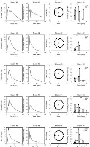
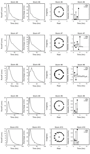
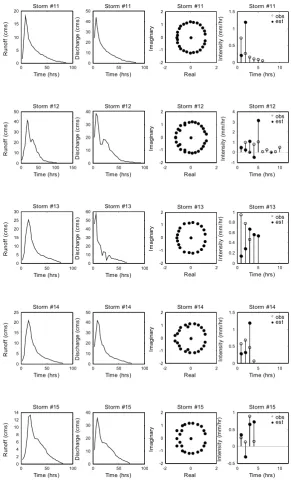
storm y22 is used to check the validity of the proposed method by showing runoff reproduction.

175

The runoff hydrographs y corresponding to the 22 different storms are shown in the leftmost panel

176

of each row in Figure 2.

177

(6)

0 50 100 0 5 10 15 20 Time (hrs) Ru no ff ( cm s) Storm #1

0 50 100

-10 0 10 20 30 40 Time (hrs) D is char ge ( cm s) Storm #1

-2 0 2

-2 -1 0 1 2 Real Im ag in ar y Storm #1

0 5 10

0 0.2 0.4 0.6 0.8 Time (hrs) In te ns ity ( m m /h r) Storm #1 ° obs • est

0 50 100

0 2 4 6 8 10 12 14 Time (hrs) R un off ( cms ) Storm #2

0 50 100

0 10 20 30 40 50 Time (hrs) D is c har ge ( cm s) Storm #2

-2 0 2

-2 -1 0 1 2 Real Ima g in a ry Storm #2

0 5 10

0 0.2 0.4 0.6 0.8 1 Time (hrs) In te n si ty ( mm/h r) Storm #2

° obs • est

0 50 100

0 5 10 15 20 Time (hrs) Ru n off ( cms ) Storm #3

0 50 100

0 10 20 30 40 Time (hrs) D is c har ge ( cm s) Storm #3

-2 0 2

0 5 10

0 0.2 0.4 0.6 0.8 1 Time (hrs) In te n si ty ( mm/ h r) Storm #3

° obs • est

0 50 100

0 5 10 15 20 25 30 Time (hrs) R uno ff (c m s) Storm #4

0 50 100

0 10 20 30 40 50 Time (hrs) D is ch ar ge ( c m s) Storm #4

-2 0 2

-2 -1 0 1 2 Real Im agi nar y Storm #4

0 5 10

0 0.2 0.4 0.6 0.8 1 1.2 1.4 Time (hrs) In tens it y (m m /hr ) Storm #4 ° obs • est

0 50 100

0 2 4 6 8 10 12 14 Time (hrs) R unof f (c m s) Storm #5

0 50 100

0 10 20 30 40 50 Time (hrs) D is ch ar ge ( c m s) Storm #5

-2 0 2

0 5 10

0 0.1 0.2 0.3 0.4 0.5 0.6 0.7 Time (hrs) In tens it y (m m /hr ) Storm #5 ° obs • est

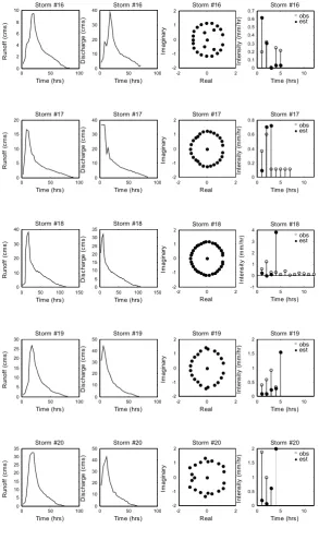
179

Figure 2. Observed runoff data (22 storms of Nenagh Basin) and the results of the root selection

180

method applying each runoff: the panels from left to right of each row plot successively the runoff

181

hydrograph, estimated unit hydrograph, Argand plot for selected roots, and hyetographs for both

182

measured and estimated rainfalls

183

(7)

0 50 100 0 5 10 15 20 Time (hrs) Ru n off ( cms ) Storm #6

0 50 100

-2 0 2

0 5 10

0 0.5 1 1.5 Storm #6 Time (hrs) In te n si ty ( mm/h

r) ° obs_•_est

0 50 100

0 5 10 15 Time (hrs) R uno ff ( cm s) Storm #7

0 50 100

0 5 10 15 20 25 30 35 Time (hrs) D is ch ar ge ( cm s) Storm #7

-2 0 2

0 5 10

-0.5 0 0.5 1

1.5 Storm #7

Time (hrs) In te ns ity ( mm/ h

r) °_{• est} obs

0 50 100 150 0 2 4 6 8 10 12 14 Time (hrs) R unof f (c m s) Storm #8

0 50 100

0 5 10 15 20 25 Time (hrs) D is ch ar ge ( cm s ) Storm #8

-2 0 2

0 5 10

-1 -0.5 0 0.5 1 1.5

2 Storm #8

Time (hrs) In tens it y (m m /hr

) _{° obs}

• est

0 50 100

0 5 10 15 20 Time (hrs) Ru n off ( cms ) Storm #9

0 50 100

-2 0 2

-2 -1 0 1 2 Real Im ag inar y Storm #9

0 5 10

0 0.2 0.4 0.6 0.8

1 Storm #9

Time (hrs) In te n si ty ( mm/ h

r) ° obs

• est

0 50 100

0 2 4 6 8 10 12 14 Time (hrs) R uno ff (c m s) Storm #10

0 50 100

0 10 20 30 40 Time (hrs) D is ch ar ge ( cm s) Storm #10

-2 0 2

0 5 10

0 0.2 0.4 0.6 0.8 Storm #10 Time (hrs) In tens ity ( m m /hr

) ° obs

• est

185

Figure 2. (Continued)

(8)

0 50 100 0 5 10 15 20 Time (hrs) R u no ff ( cms ) Storm #11

0 50 100

0 10 20 30 40 50 Time (hrs) D is char ge ( cm s ) Storm #11

-2 0 2

-2 -1 0 1 2 Real Im a gi n ar y Storm #11

0 5 10

0 0.5 1

1.5 Storm #11

Time (hrs) In te ns ity ( m m /h

r) ° obs

• est

0 50 100 150 0 10 20 30 40 50 Time (hrs) Ru n off ( cms ) Storm #12

0 50 100

0 10 20 30 40 Time (hrs) D is char ge ( cm s ) Storm #12

-2 0 2

-2 -1 0 1 2 Real Ima gi n ar y Storm #12

0 5 10

-1 0 1 2 3

4 Storm #12

Time (hrs) In te ns ity ( mm/h

r) °_{• est} obs

0 50 100

0 5 10 15 20 25 30 Time (hrs) Ru n off ( cms ) Storm #13

0 50 100

0 10 20 30 40 50 60 Time (hrs) D is c har ge ( cm s) Storm #13

-2 0 2

0 5 10

0 0.2 0.4 0.6 0.8

1 Storm #13

Time (hrs) In te n si ty ( mm/h

r) ° obs

• est

0 50 100

0 5 10 15 20 25 Time (hrs) R uno ff ( cm s) Storm #14

0 50 100

0 10 20 30 40 50 Time (hrs) D is ch ar ge ( cm s) Storm #14

-2 0 2

0 5 10

0 0.5 1 1.5 Storm #14 Time (hrs) In te ns it y ( mm/ h

r) ° obs_•_est

0 50 100

0 2 4 6 8 10 12 14 Time (hrs) R unof f (c m s) Storm #15

0 50 100

0 10 20 30 40 Time (hrs) D is ch ar ge ( c m s) Storm #15

-2 0 2

0 5 10

-0.5 0 0.5

1 Storm #15

Time (hrs) In tens it y (m m /hr

) ° obs

• est

187

(9)

0 50 100 0 2 4 6 8 10 Time (hrs) Ru n off ( cms ) Storm #16

0 50 100

0 10 20 30 40 Time (hrs) D is c har ge ( cm s) Storm #16

-2 0 2

0 5 10

0 0.1 0.2 0.3 0.4 0.5 0.6

0.7 Storm #16

Time (hrs) In tens ity ( m m /hr

) ° obs

• est

0 50 100

0 5 10 15 20 Time (hrs) R u nof f (c m s) Storm #17

0 50 100

0 10 20 30 40 Time (hrs) D is char g e (c m s) Storm #17

-2 0 2

-2 -1 0 1 2 Real Ima gi n ar y Storm #17

0 5 10

0 0.2 0.4 0.6

0.8 Storm #17

Time (hrs) In te n si ty ( mm/h

r) ° obs_{• est}

0 50 100 150 0 10 20 30 40 Time (hrs) R unof f ( cm s) Storm #18

0 50 100 150 0 5 10 15 20 25 30 35 Time (hrs) D isch a rg e ( cms) Storm #18

-2 0 2

0 5 10

-1 0 1 2 3

4 Storm #18

Time (hrs) In te ns it y ( m m /h

r) ° obs_•_est

0 50 100

0 5 10 15 20 25 30 Time (hrs) R uno ff ( cm s) Storm #19

0 50 100

0 10 20 30 40 50 Time (hrs) D is ch ar ge ( cm s ) Storm #19

-2 0 2

0 5 10

0 0.5 1 1.5

2 Storm #19

Time (hrs) In tens it y ( m m /hr

) ° obs

• est

0 50 100

0 5 10 15 20 25 30 35 Time (hrs) Ru n off ( cms ) Storm #20

0 50 100

-2 0 2

0 5 10

0 0.5 1 1.5 2 Storm #20 Time (hrs) In tens ity ( m m /hr

) ° obs

• est

189

(10)

0 50 100 0

10 20 30 40 50 60

Time (hrs)

R

uno

ff

(

cm

s)

Storm #21

0 50 100

0 10 20 30 40

Time (hrs)

D

is

ch

ar

ge (

cm

s)

Storm #21

-2 0 2

-2 -1 0 1 2

Real

Im

agi

nar

y

Storm #21

0 5 10

-2 0 2 4

6 Storm #21

Time (hrs)

In

te

ns

ity

(

m

/h

r) _° obs

• est

0 50 100

0 5 10 15 20 25

Time (hrs)

R

u

no

ff (

cms

)

Storm #22

0 50 100

0 10 20 30 40

Time (hrs)

D

is

char

ge (

cm

s)

Storm #22

-2 0 2

-2 -1 0 1 2

Real

Im

ag

in

ar

y

Storm #22

0 5 10

-1 0 1 2

3 Storm #22

Time (hrs)

In

te

ns

ity

(

m

/hr

) _°_obs

• est

191

192

The UHs h_m (m=1,, 22) were derived individually from the 22 different storm events by the

193

conventional root selection method. The resulting UHs and roots of H zm( −1) for corresponding

194

storm events are indicated in the second and third panels from left of each row in Figure 2. It appears

195

that the root patterns for many different storm events are fairly displaced from the regular pattern,

196

resulting in fluctuations of ordinates in many UHs. Therefore, it could be supposed that the

197

individual UHs are virtually subject to uncertainty related with the randomness. Each rightmost

198

panel in the rows of Figure 2 shows the rainfall difference between the values from measured

199

hyetograph and the roots from X zm( −1), m=1, , 22 . One sees the presence of inevitable and

200

remarkable discrepancy in estimated rainfall in many storms. This indicates clearly that the

201

uncertainty in runoff data affected the estimation of both rainfall and UHs.

202

To clarify the uncertainties in UHs, Figure 3(a) shows a plot in which the 22-individual storm

203

UHs are stacked altogether, and Figure 3(b) plots the Argand diagrams of the corresponding

204

( 1, , 22) m

Y m₌  . Figure 3(a) reveals the large variation between UHs, the significant oscillations of

205

the ordinates values, and the abnormal ordinate values as well. Thus, if a representative UH is

206

derived based on these UHs, this representative UH might be subjected to high variation related to

207

uncertainties. Even though not all individual Argand diagrams show perfect circular pattern of

208

runoff roots as shown in Figure 1, the stacked Argand diagrams in Figure 3(b) show explicit circular

209

pattern of the runoff roots. Thus, stacking the runoff data permits to identify more easily the

210

abnormal roots from the runoff roots.

211

0 50 100

-10 0 10 20 30 40 50 60

Time (hrs)

R

unof

f (

cm

s)

(a)

-2 -1 0 1 2

Real

Im

aginar

y

(b)

212

Figure 3. Applying root selection method in conventional way to 22 storms of Nenagh Basin: (a)

213

estimated unit hydrographs by root selection method; (b) Argand plot for runoff polynomials.

214

(11)

The Savitzky-Golay filtering was applied to the 22 runoffs. To produce single smoothed runoff y*,

216

the filter used adjacent five runoff ordinate values as introduced in Equation 2. Figure 4(a) shows the

217

UH stacking the 22 different storms after the Savitzky-Golay filtering and Figure 4(b) indicates the

218

Argand diagrams for corresponding Y_m* (m₌1,, 22).

219

220

0 50 100

-10 0 10 20 30 40 50 60

Time (hrs)

R

unof

f (

cm

s)

(a)

-2 -1 0 1 2

Real

Im

aginar

y

(b)

221

Figure 4. Effect of applying Savitzky-Golay filter to 22 storms of Nenagh Basin: (a) estimated unit

222

hydrographs by root selection method; (b) Argand plot for runoff polynomials.

223

In Figure 4(a), one can observe that the variations among the ordinates of each UH are fairly reduced

224

compared to Figure 3(a). Moreover, the overall pattern of UH root circles based on the filtered data

225

shown in Figure 4(b) appears to be improved in the sense that the roots in the circular pattern gets

226

closer together when using the Savitzky-Golay filter. The result shows that the Savitzky-Golay filter

227

stabilizes the UH by reducing the uncertainty brought by the random error from the runoff data.

228

Besides, compelling changes related with abnormal roots can be found. The abnormal points,

229

positioned outside the circle in Figure 3(b), are repositioned inside the circle after smoothing as in

230

Figure 4(b), while the abnormal points inside the circle virtually retain their position. However, this

231

change of root pattern did not contribute in producing a better rainfall estimate.

232

233

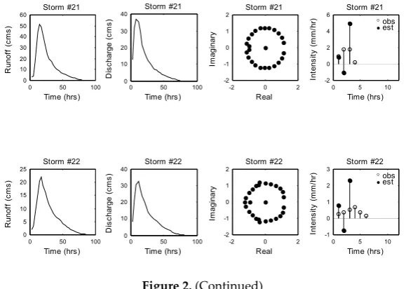
3.2 Evaluation Using the Performance Index

234

In order to investigate the effect of the Savitzky-Golay filter more precisely, this study

235

compared the performance of UHs with/without Savitzky-Golay filtering. Among the numerous

236

goodness-of-fit criteria, this study selected the Nash-Sutcliffe model efficiency coefficient [13] as

237

comparison index following the recommendation of ASCE [14]. The Nash-Sutcliffe index is defined

238

as:

239

(

)

(

)

2

1

2

1

ˆ 1

n

i i

i n

i i

y y

E

y y

=

 

−

 

= −_ _

 ₋ 

 

 



, (9)

in which yi is the observed runoff; yˆi is the modelled discharge; and, y is the average

240

discharge at time t. The closer the Nash-Sutcliffe index to 1, the better the performance of the model.

241

Specifically, a value of 0.9 for E indicates a very satisfactory model performance, a value between 0.8

242

and 0.9 indicates an acceptable model, and a value between 0.6 and 0.8 indicates unsatisfactory

243

fitting results [15]. The applicability of UHs were compared using the Nash-Sutcliffe index for UH

244

models with and without Savitzky-Golay filtering. Table 1 compares the Nash-Sutcliffe index

245

yielded for the 22 storms of Nenagh basin. The last row in the table represents the average value for

246

both UHs.

247

(12)

Table 1. Comparison of Nash-Sutcliffe model efficiency coefficient for UHs with/without

249

Savitzky-Golay filtering.

250

251

252

The table apparently indicates that for most of the events, the UH model with filtering performs

253

better than the UH without filtering. The overall index value clearly proves the applicability of

254

Savitzky-Golay filtering as indicated by the average Nash-Sutcliffe index of 0.83 (> 0.8). This result

255

shows that the UH model using Savitzky-Golay filtering can be recommended for the prediction of

256

rainfall-runoff of the Nenagh basin at least.

257

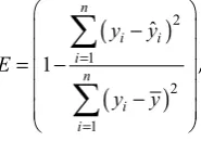
3.3 Deriving of Optimal UH (Multiple-Event Analysis)

258

The 22 storms presented chronologically in Figure 2 were used for deriving an optimal UH. For

259

this purpose, the first 21 storms were used to give an optimal UH estimate with careful selection of

260

the abnormal roots on the basis of Figure 4. The last 22nd storm was used for validation of the

261

prediction. Using each of the 21 single-event UHs H z_m( −1), m=1,, 21, a multiple-event UH

262

1

( )

H z− was derived by the linear combination method as shown in Equation (7). The optimal UH

263

1

( )

H z− is compared to a selection of H zm( −1), m=1, 2, 10, 16 in Figure 5. In the figure, the UHs

264

based on the selected storms vary from one storm event to another.

265

Event Nash-Sutcliffe model efficiency coefficient

Without filter With filter

1 .59 .84

2 .65 .97

3 .89 .88

4 .65 .77

5 .56 .76

6 -.01 .68

7 .58 .73

8 .85 .84

9 .88 .78

10 .96 .97

11 .89 .93

12 .88 .87

13 .09 .95

14 .93 .98

15 .88 .99

16 .73 .69

17 .85 .85

18 .48 .62

19 .27 .73

20 .09 .60

21 .91 .95

22 .93 .90

(13)

0 10 20 30 40 50 60 70 80 90

Time (hr)

0 5 10 15 20 25 30 35 40

peak ordinate of optimal UH

optimal UH UH storm 1 UH storm 2 UH storm 10 UH storm 16 UH (Bree, 1978)

266

Figure 5. Comparison of UH ordinates obtained by this research (optimal UH) with those of selected

267

events and Bree [10].

268

These selected storms were also used by Bree [10] to obtain a reliable UH when using the least

269

squares method. According to Bree [10], the estimation of the UH from a single-event analysis did

270

not result in a reliable UH. Besides, the combination of multiple storms produced more reliable UH

271

by reducing the oscillations of UH ordinates. Similar result could be observed in this research. In

272

Figure 5, one can find that the oscillations in the individual UHs H z_m( −1) were virtually removed

273

when the multiple-event analysis was applied. Thus, to calculate a design runoff in conjunction with

274

a design rainfall, using multiple-event UH H z( −1) is preferable for better prediction.

275

3.4 Estimating Parameters of Nash’s IUH

276

The parameters (n, K) for available storms in Nenagh basin were determined by MOM which

277

uses the single-event UH for each storm and corresponding unit rainfall provided with 1 cm depth

278

for 3-hours duration. For this calculation, a computer code serviced by Colorado State University

279

[16] was used. Incidentally, Mohan and Vijayalakshmi [11] have carefully determined the Nash’s

280

parameters based on a typical MOM procedure using rainfall data. Thus, the parameter values given

281

by Mohan and Vijayalakshmi [11] could provide proper reference values to be compared with those

282

resulting from this research. Table 2 lists the parameters (n, K) for 21 storms obtained from these two

283

different approaches.

284

285

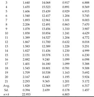
Table 2. Comparison of Nash IUH’s parameters of this research with those of Mohan and

286

Vijayalakshmi [11].

287

Event This research Mohan and

Vijayalakshmi (2008)

n k n k

1 1.955 14.293 0.996 7.926

(14)

3 1.640 14.068 0.917 6.888

4 1.655 15.523 0.891 8.569

5 1.606 15.439 0.929 6.915

6 1.540 12.417 1.204 5.745

7 1.893 12.961 1.101 8.003

8 2.206 12.491 0.863 7.670

9 1.078 13.456 1.310 3.907

10 1.858 10.854 1.241 4.629

11 1.389 14.527 1.204 4.772

12 1.867 11.700 0.632 8.018

13 1.583 12.389 1.228 5.251

14 1.827 11.436 1.230 4.999

15 2.151 10.578 1.151 6.230

16 2.882 9.240 1.099 6.098

17 1.401 16.180 1.099 5.388

18 1.545 18.801 0.781 9.308

19 1.709 10.538 1.163 5.692

20 2.167 8.443 1.195 5.924 21 2.293 9.365 1.201 5.172 Avg. 1.828 12.568 1.077 6.317 Sd. 0.394 2.659 0.178 1.457

n k× 22.953 6.803

288

Table 2 also indicates the statistical properties featuring the variation of the determined

289

parameters. It can be seen that the result obtained in this study exhibit fairly higher values in both

290

parameters than those of the reference values. However, the degree of variation of these values can

291

be regarded as being low in view of the small values of the standard variations. The product values

292

of n and K (n K× ) for all storms were considered to be constant with an average of 22.953, which is

293

significantly higher than the reference value of 6.803. Thus, the IUH with the parameter values of

294

this study would produce lower peak discharge and more delayed time-to-peak in comparison to

295

the IUH given by Mohan and Vijayalakshmi [11]. However, it is evident that the IUH obtained from

296

the root selection would be able to predict runoff more accurately by transferring a few number of

297

UH roots into rainfall roots. Therefore, future work should focus on the efficiency of the selection

298

procedure for UH roots.

299

3.5 Predicted Runoff Using the Optimal UH

300

Event 22 was used to verify the optimal UH H zˆ ( )−1 estimated from 21 storms. Figure 6

301

compares the observed and predicted runoffs using the optimal UH. The single-event UH H22(z−1)

302

derived by the root selection method is also plotted in Figure 6.

303

(15)

0 10 20 30 40 50 60 70 80 90 100 0

1

2

3

4

5

6

7

8

9

10

P

rec

ipit

at

io

n (

m

)

Time (hr)

storm # 22

0 10 20 30 40 50 60 70 80 90 100 0 5 10 15 20 25 30

D

is

char

ge (

cm

s)

rainfall depth predicted reproduced observed

305

Figure 6. Comparison between the runoff predicted for 22nd storm using the optimal unit

306

hydrograph obtained from 21 storms and the runoff reproduced using the single event unit

307

hydrograph for 22nd event, and the observed runoff for 22nd storm event.

308

In Figure 6, there is no remarkable difference in the overall shape between the observed and

309

predicted runoffs. The peak discharge of the predicted runoff agrees well with that of the observed

310

one. However, the optimal UH resulted in a slightly larger value of the time-to-peak in the predicted

311

runoff. This problem might be solved by selecting more abnormal roots from the runoff roots to

312

reform the optimal UH to another optimal UH having smaller number of ordinates. However, this

313

method involves more subjectivity in the root selection procedure.

314

Interestingly, the reproduced hydrograph using the single-event UH H22(z−1)shows larger

315

deviation from the observed runoff compared to the predicted hydrograph using the optimal UH.

316

This is mainly due to higher uncertainty associated with the determination of H22(z−1). This

317

strongly suggests that using multiple-event UH along with runoff filtering would be applicable

318

especially in absence of rainfall data.

319

320

4. Conclusion

321

The root selection method can be used for determining a UH when rainfall data are not

322

available. The root selection method has shown successful results, but the uncertainty related to

323

noise fluctuations in the resulting UH remains unclear yet. The determination of an optimal UH

324

(multiple-event UH) based on available UHs individually obtained from many storm events

325

(single-event UH) is an important problem for practical use. This study proposed an improved root

326

selection method based on the smoothing technique using the Savitzky-Golay filter to reduce

327

significantly the noise fluctuations in runoff data. The proposed method provided single-event UH

328

for each storm with better applicability. This paper also focused on deriving the optimal UH by

329

linear combination of the single-event UHs from different storms. In addition, determination of

330

(16)

proposed method was applied to twenty-two storm events for a basin of the Nenagh River at

332

Claianna, Ireland.

333

In most storm events, the values of Nash-Sutcliffe index using the UHs obtained from the

334

existing root selection method reached unacceptable level (less than 0.8). However, the values of

335

Nash-Sutcliffe index using the UHs based on filtered runoff data appeared to be satisfactory with

336

values higher than 0.8. This result proved that the application of the Savitzky-Golay filter in root

337

selection method enables more accurate prediction by reducing the uncertainty associated with

338

fluctuations of ordinates in runoff data.

339

The proposed method yielded a non-biased estimation of the optimal UH in the sense that the

340

storms with larger runoff and the storms with smaller runoff equally contributed to the

341

determination of the optimal UH. The fluctuations found in some single-event UHs were virtually

342

removed in the optimal UH, and a validation result indicated that there was no remarkable

343

difference between the optimal UH and the UH obtained by using rainfall data.

344

Using the root selection method along with the method of moments allowed the estimation of

345

the parameters of Nash’s IUH. However, it was shown that the IUH with these parameters would

346

result in slightly lower peak values. An objective method to reduce the number of ordinates in UH is

347

necessary.

348

To the knowledge of the author, the proposed root selection method in this research provided a

349

fairly enhanced result in estimating UH for practical use even though few important problems

350

remained to be solved. The proposed method can potentially be applied to other hydrological

351

analysis even when using rainfall data.

352

5. Patents

353

Acknowledgment: This research was fully funded by a Konkuk University Research Committee grant.

354

References

355

1. De Laine, R. J. Deriving the unitgraph without using rainfall data. J. Hydrol. 1970, 10, 379–390,

356

doi:10.1016/0022-1694(70)90224-6.

357

2. Turner, J. E.; Dooge, J. C. I.; Bree, T. Deriving the unit hydrograph by root selection. J. Hydrol.1989, 110,

358

137–152, doi:10.1016/0022-1694(89)90240-0.

359

3. Ojha, C. S. P.; Singh, K. K.; Verma, D. V. S. Single-Storm Runoff Analysis Using Z-Transform. J. Hydrol.

360

Eng.1999, 4, 80–82, doi:10.1061/(ASCE)1084-0699(1999)4:1(80).

361

4. Parmentier, B.; Dooge, J. C. I.; Bruen, M. Root selection methods in flood analysis. Hydrol. Earth Syst. Sci.

362

2003, 7, 151–161, doi:10.5194/hess-7-151-2003.

363

5. Bruen, M.; Dooge James; Parmentier, B. Root-selection methods for separating the urban and rural

364

components of flood hydrographs in urbanising catchments. In Water in the Celtic world: managing resources

365

for the 21th century; British Hydrological Society: Aberystwyth, 2000; pp. 173–180.

366

6. Seong, K. W.; Lee, Y. H. A practical estimation of Clark IUH parameters using root selection and linear

367

programming. Hydrol. Process.2011, 25, 3676–3687, doi:10.1002/hyp.8094.

368

7. Turner, J. E.; Dooge, J. C. .; Bree, T. Comment on “Single storm runoff analysis using Z-transform”;

369

J.Hydrol.Eng.2001, 6, 173–174.

370

8. Savitzky, A.; Golay, M. J. E. Smoothing and Differentiation of Data by Simplified Least Squares

371

Procedures. Anal. Chem.1964, 36, 1627–1639, doi:10.1021/ac60214a047.

372

9. Chau, F. Chemometrics : from basics to wavelet transform; Wiley-Interscience, 2004; ISBN 0471454737.

373

10. Bree, T. The stability of parameter estimation in the general linear model. J. Hydrol.1978, 37, 47–66,

374

doi:10.1016/0022-1694(78)90095-1.

(17)

11. Mohan, S.; Vijayalakshmi, D. P. Estimation of Nash’s IUH parameters using stochastic search algorithms.

376

Hydrol. Process.2008, 22, 3507–3522, doi:10.1002/hyp.6954.

377

12. Nash, J. E. The form of the instantaneous unit hydrograph. Int. Assoc. Sci. Hydrol.1957, 45, 114–121.

378

13. Nash, J. E.; Sutcliffe, J. V River flow forecasting through conceptual models part I — A discussion of

379

principles. J. Hydrol.1970, 10, 282–290, doi:10.1016/0022-1694(70)90255-6.

380

14. Yen, B. C.; ASCE Task Committee on Definition of Criteria for Evaluation of Watershed Models of the

381

Watershed Management Committee Irrigation and Drainage Division Discussion and Closure: Criteria

382

for Evaluation of Watershed Models. J. Irrig. Drain. Eng.1995, 121, 130–132.

383

15. Jagan Mohan Reddy, A.; Suresh Babu, C.; Mallikarjuna, P.; Reddy, J. M.; Suresh Babu, A.; Mallikarjuna, C.

384

Rainfall – Runoff Modeling: Comparison and Combination of Simple Time-Series, Linear Autoregressive

385

and Artificial Neural Network Models. WSEAS Trans. Fluid Mech.2008, 3, 126–136.

386

16. RAMÍREZ, J. A. Colorado State University Available online:

387

http://www.engr.colostate.edu/~ramirez/ce_old/classes/ (accessed on Oct 10, 2017).

Creative Commons CC BY