A Game Theoretic Resource Allocation Model
Based on Extended Second Price Sealed Auction
in Grid Computing
Weifeng Sun
School of Software, Dalian University of Technology, Dalian, China Email: [email protected]
Qiufen Xia, Zichuan Xu, Mingchu Li, Zhenquan Qin School of Software, Dalian University of Technology, Dalian, China
Email: {xiaqiufen, zichuanxu.mail}@gmail.com, [email protected], [email protected]
Abstract—In resource-limited environment, grid users compete for limited resources, and how to guarantee tasks’ victorious probabilities is one of the most primary issues that a resource scheduling model cares. In order to guarantee higher task’s victorious probabilities in grid resources scheduling situations, a novel model, namely ESPSA (Extended Second Price Sealed Auction), is proposed. The ESPSA model introduces an analyst entity, and designs analyst’s prediction algorithm based on Hidden Markov Model (HMM). In ESPSA model, grid resources are sold through second price sealed auction. Moreover, to achieve high victorious probabilities, the user brokers who are qualified to participate in the auctions will predict other players’ bids and then carry out the most beneficial bids. The ESPSA model is simulated based on GridSim toolkit. Simulation results show that the ESPSA model assures a higher victorious probability and superior to other traditional algorithms. Moreover, we analyze the existence of Nash equilibrium based on simulation results, thus, any participant who changes its strategy unilaterally could not make the results better.
Index Terms—grid resource scheduling, game theory, extended second price sealed auction
I. INTRODUCTION
The concept of grid technology originates from electricity grid. Idle resources in grids are connected through internet and grid users can access the resources no matter where they are. Grid system is heterogeneous, multi-zone managed, large-scale and distributed. Furthermore, grid system is concerned with a dynamic collection of diverse resources and services across multiple domains, and resources apply and demand is dynamic either. As resources join and exit dynamically, the loads of grid resources change continuously. All these characteristics show that grid system needs a dynamic and high-efficiency resources scheduling algorithm, which can manage dynamic resources flexibly.
The majority of grid systems fall in the category of resource-rich ones, where resources compete for limited tasks. However, sometimes, numerous tasks are submitted at the same time, leading to the undersupplying of resources, which makes tasks compete for limited resources. Whether tasks compete for resources or resources compete for tasks, the resources providers will benefit from assigning resources and the thing that users need to do is paying for the resources. Thus, it is reasonable to model the resource scheduling by economic models. However, current literature on economic grid models only limits to the basic auction models where the bidders bid according to a single factor. Some algorithms integrate simple prediction methods into the bidding algorithms without assuring the victorious probability. Thus, with the increase of the complexity of grid systems, how to improve those simple bidding strategies, prediction algorithms and victorious probability is becoming urgent.
This paper is an extension in terms of both theoretic and simulation results of our conference paper [1]. The major contributions of this paper are as follows.
y To solve the task’s low victorious probability problems using game theory in grid resource scheduling situations, an ESPSA (Extended Second Price Sealed Auction, ESPSA) model is proposed in this paper. An analyst entity is introduced in the model to fulfill the trend that roles in grids are increasing dramatically.
y The ESPSA model extends second price sealed auction mechanism. In the extended auction, the total price is sealed while keep the resource demand quantity unsealed.
y This paper introduces a prediction algorithm based on Hidden Markov Model, improves basic bidding algorithms and increases participants’ victorious probability.
y GridSim toolkit is utilized to simulate the algorithms and the existence of Nash equilibrium is analyzed, and then proved theoretically. The rest of paper is organized as follows: section II is the related work; section III describes the ESPSA model;
section IV elaborates the simulation and analyzes the simulation results and the computational load of the ESPSA, also the existence of Nash Equilibrium is proved theoretically in this part. Section V draws the conclusion and discusses about the future work.
II. RELATED WORK
At present, resources management and dynamic scheduling based on game theory is becoming a focus of researches in the settings of P2P, grid and cloud computing. A lot of work has been done by researchers, and it will be overviewed in this section from the perspective of grid and cloud computing.
Game theoretic methods have been adopted in settings of cloud and grid computing. In the first place, from the grid computing perspective, Lei Yao and Guanzhong Dai (2008) [2] focus on resource-rich environment. They propose a method, namely GVP, which could guarantee resources’ victorious probabilities. In their method, resources win the auction by predicting other resources’ bids based on the mean value of historical bids. However, the prediction algorithm is too simple to get accurate predictions. Maheswaran and Basar(2003) [3] discuss a divisible auction and adopts a decentralized strategy, but users only make decisions according to resources’ historical load information without consideration of the changing trend of resources’ loads. Kwok and Song (2005) [4] propose a hierarchical grid model, in which resources are selfish. The selfishness of resources makes them only consider their own needs when executing tasks. This kind of action delays tasks’ execution even though the tasks could accurately predict their opponents’ bids. This model couldn’t guarantee tasks’ victorious probabilities. Bredin and Kotz (2003) [5] propose a resources allocation algorithm based on mobile brokers’ competing for resources. In this model, user brokers make an inaccurate prediction for resources, and they neglect the prediction of other user brokers’ behavior. LI Zhijie and Cheng Chuntian (2006) [6] propose a resource allocation model that uses sequential game to predict resource load for time optimization. In this model, user brokers offer their bids in sequence, causing first-mover advantage, which makes the model less popular in practical applications. Abramson and Buyya (2002) [7] propose grid resource scheduling model which only considers the relationship between users and resources without considering the interactions between users. Thus, this model is too idealized to be used in practical circumstances.
Game theoretic solutions also attracted a lot researchers’ attention in the research area of cloud computing [ 8, 9, 10, 11, 12, 13, 14, 15]. Chonho, et al. (2010) [12] study an evolutionary game theoretic mechanism for adaptive and stable application deployment in cloud computing settings. Their algorithm, called Nuage, allows applications to adapt their locations and resource allocation to the environmental conditions in a cloud. Wei,G., et al. (2010) [13] consider a QoS constrained resource allocation problem, in which service demanders try to solve sophisticated parallel computing
problem. Their solution consists of two steps. First, each participant solves its optimal problem independently, without consideration of the multiplexing of resource assignments. Then, an evolutionary mechanism which takes both optimization and fairness into account is designed. Rajkumar Buyya and Manzur Murshed (2002) [14] present a game theoretic method to schedule dependent computational cloud computing services and an evolutionary mechanism is designed. Fei and Frederic (2010) [15] introduce a new Bayesian Nash Equilibrium Allocation algorithm to solve resource management problem in cloud computing. Through experiments, they show that cloud users can receive Nash equilibrium allocation solutions by gambling stage by stage and the resource will converge to the optimal price.
The impact of selfish behavior entities has been paid a lot of attention in self-organized Mobile Ad hoc Networks (MANNEs) and Peer-to-Peer (P2P) networks [16, 17, 18, 19, 20, 23, 24, 25]. In such networks, each node specified as player is under the authority of a self-interested user.
All the literatures [2-25] listed above have made remarkable contributions to economic resources scheduling and allocation algorithm in the settings of grid and cloud computing, but some of them have a low accuracy prediction method for agents to predict tasks’ bids. In response to these issues, a model, namely ESPSA, based on extended second price sealed auction and Hidden Markov Chain prediction method is proposed. In ESPSA model, a mass of tasks compete for limited resources, and tasks decide their best bidding price according to their resource demand quantities, their budgets and predictions of their opponents’ bids. In this way, the ESPSA model will guarantee the tasks a higher victory probability when competing for grid and cloud resources than other methods do in the above literatures.
III. ESPSARESOURCE ALLOCATION MODEL AND
ALGORITHM
The ESPSA model [1] is consisted of extended second price auction algorithm, resource broker’s algorithm, user broker’s algorithm with HMM. Specifically, the extended second price auction sealed the total price of each trade and unsealed the resource demand quantity. By invoking the extended auction, the users’ and resources’ brokers represent as bidders and auctioneers respectively.
As Figure 1 shows, when a user wants to execute some tasks, it sends the task list to a user brokerUBi. After
receiving the task list, in order to be qualified to take part in an auction, UBi sends an application message with its
expected victorious probability and amount of resource that it demands to resource broker RBi . If resource
broker RBi agrees UBi to take part in the auction, UBi
sends prediction request to an Analyst. On receiving the predictions, UBi calculates its bid according to the
prediction results. After that, it will send its bid to RBi.
Finally, RBi sends winners to UBi and resource demand
quantity of UBi to information service entity.
One of the improvements of our model is the analyst entity that we proposed. An analyst gets information from the information service entity, and provides prediction services to user brokers. The analyst entity’s prediction algorithm is based on HMM. Obviously, it satisfies the trend that roles in grids are increasing dramatically and makes the market model of grids computing much more practical.
Figure 1. ESPSA model
The detailed user broker algorithm, resource broker algorithm and ESPSA prediction algorithm are described in section A, B and C respectively.
A. Algorithm of Resource Broker
As described above, ESPSA considers a resource-limited grid model where resource brokers need to act as auctioneers who invoke auctions among user brokers. For a resource broker, if it makes a higher expected profit for resources, it will be favored by the resources. Thus, the resource broker should limit the number of the bidders in order to fulfill most of the bidders’ expected victorious probability in one round auction.
We propose a method which classifies the Sbidder into
two sets: u bidder
S and Sbidderv represent users with an
expected victory probability which is higher or lower than the basic victory probability set by the model respectively.
TABLE I.
RESOURCE BROKER’S ALGORITHM
Algorithm Name Resource Broker’s algorithm Input: A set of Bidders who expect to take
part in the auction (Sbidder), bidders’ expected victorious probability
{ }
Prwini and bidders’
bids.
Output: Messages that invoking a auction and winning messages. 1.Classify the bidders into u
bidder S and v
bidder
S according to the user’s task’s average tasks’
2.Invoke the first round auction where the bidders are in the set u
bidder
S .
3.Waiting until received the bidding information
(
)
{
bij,dij}
from user brokers.4.Calculate each user broker’s the unit price by ij ij ij
r =b d . Set the user broker with highest rij as the winner.
5.Send need vector Dj =
{
d1j,d2j,…dij,…,dnj}
toInformation Service Entity (shown in Figure.1). 6.If min(Pr )win Prwin
i > RB . Invoke a new auction where the bidders are in the set v
bidder
S .
7.Else, rank v bidder
S by the resource demand amount in increasing order. Add the top 1 Prwin
RB users to the new set
bidder
S′ . Invoke a new auction where the bidders are the new set Sbidder′ .
8.Waiting until received the bidding information
(
)
{
bij,dij}
from user brokers.9.Calculate each user broker’s the unit price by ij ij ij
r =b d . Set the user broker with highest rij as the winner.
10.If there were any request, then start another auction round. Else, exit.
The number of bidders in each round should be calculated by Eq.(1).
,in the 1st round auction and min(Pr ) Pr 1 Pr ,else cases in 1st round
,in the 2nd round auction
u win win
bidder i RB
win bidder RB
v bidder
S
n
S
⎧ >
⎪⎪ = ⎨ ⎪ ⎪⎩
(1)
where Prwin
i specifies the expected victorious probability
of user broker UBi , and Pr win
RB represents the basic
victorious probability that resource broker RB assures.
The specific algorithm of resource broker RBi is
described in Table I.
B. Algorithm of User Broker
predict other user brokers’ bids to get a high victorious probability by using the predicting services provided by an analyst.
Specifically, a user broker calculates its primitive bid by Eq.(2)[1].
i i
b L γ
′ = (2)
Where bi′is a user broker’s primitive bid, L is the load
status of the resource and γi is a weighting factor
(i=1, 2, , ,… …i n).
TABLE II.
USER BROKER’S ALGORITHM Algorithm: User Broker’s algorithm
Input: A task set T from user.
Output: Bid
i
b
1. Firstly, user broker should apply to join in the auction. Send the applying request along with its expected victorious probability and deadline.
2. If the user broker is divided into the urgent one, then join auction, go to step 3. Else, wait for the second auction, go to step 3.
3.Calculate the primitive bid by Eq.(2) 4.Send predicting request to an analyst.
5.Waiting until received the predicting information i pre
B− from the analyst.
6.Adjust the bid by Eq.(3).
Then, UBi sends a predicting request to the analyst
and gets a set of other user brokers’ bids i pre
B− . After that,
i
UB adjusts its bid according to Eq.(3).
{ }
(
)
(
{ }
)
max i , max i
i pre i i pre
i i
b B if b B
b
b else
ε α
− −
⎧ ′ ∪ + > ′ ∪
⎪ = ⎨ ′
⎪⎩ (3)
Where αiis a user broker’s budget in one round of the
auction. biis the calculated bid of a user broker.
The user agents’ algorithm is listed in Table II.
C. ESPSA Model’s Prediction Algorithm
In ESPSA model, the entity of analyst based on HMM prediction model is introduced. In our HMM prediction model, we use the Viterbi Algorithm[26].
In HMM prediction model, hidden states couldn’t be got directly, but they can be deduced by observation sequences. In general, λ=
(
A B, ,π)
can be used torepresent a HMM, where A represents a transition
probability between initial states, B represents
observation sequence, π represents initial states matrix. Given the definitions of A, Band π , the HMM can
generate a hidden sequence: O=O O O1, 2, 3, ,… On.
In ESPSA model, the resource demand quantities and bids that are submitted by user brokers correspond to observation sequence and hidden states respectively. When an auction launched, each resource broker
publishes its attributes, such as process elements’ computing capacity, load status and so on. Each user broker can get the attributes. And then, user brokers use observed resource demand quantities
{
1 , 2 , , ,}
j j j ij nj
D = d d …d … d to predict their rivals’ bids in
next round auction: bj =
{
b1j,b2j,…bij, ,… bnj}
. dijis thedemand quantity that user broker iof resource j, bij is
the bid price of user broker ifor resource j. We take
five bids for examples, written as level1_bidding, level2_bidding, level3_bidding, level4_bidding and level5_bidding respectively, which correspond to the zones of
(
0,b1]
,(
b b1, 2]
,(
b b2, 3]
,(
b b3, 4]
,(
b b4, 5]
, wherek
b is a bid, k=1, 2,3, 4,5.
At timet, for useri, its bid for resource j isbijt , and
its resource demand quantity for j is t ij
d . Suppose that
there were n resources in grid system, according to
HMM, the initial states at time tare:
(
1, 2, , , ,)
t t t t
i i ij in
states b b b b
π = = … … (4)
And at timet, the resource demand quantity matrix
that user broker iobserves other user brokers’ is:
(
1, 2, , , ,)
t t t t
i i ii in
B=observations= d d … d … d (5)
The transition matrix from hidden states at time t−1
to hidden states at time t is:
1
1 1
1
11 1
1 A = transition _ probability =
t t
i in
t i
t in
b b
b
b
t t
i i n
t t
in inn
p p
p p
−
−
⎛ ⎞
⎜ ⎟
⎜ ⎟
⎜ ⎟
⎜ ⎟
⎝ ⎠
…
(6)
The emission matrix between observation sequences and hidden states is:
11 1
1
_ 1 _
_ 1
ta_ _ probability=
t t
n
t t
n nn
obs obs n
sta
s n
p p
emission
p p
⎛ ⎞
⎜ ⎟
⎜ ⎟
⎜ ⎟
⎝ ⎠
…
(7)
where t ij
p represents the probability of obs_j when in
state sta_i at time t, i=1, 2, ,… n, j=1, 2, ,… n.
IV. SIMULATION AND RESULTS ANALYSIS
The GridSim toolkit [23] is utilized in the simulation of this paper. Resource entities, user entities, broker entities and information about resource demand are considered.
A. Expriment Setup
It is necessary to make some initial setting reasonable by training especially the parameters used in HMM. There exist 300 resources in the resource queue, which means the user brokers may take part in at most 300 auctions. Table III lists the properties of the four resources.
TABLE III.
CHARACTERISTICS OF GRID RESOURCES IN GRIDSIM Name Resource
characteristics
PE number
A PE MIPS rating
Transmitting Rate
0
R Sun Ultra, Solaris 2 320 2000MB/s 1
R Sun Ultra, Solaris 4 350 2000MB/s 2
R Intel Pentium
Linux
1 370 2500MB/s
3
R Intel Pentium
Linux
3 390 2500MB/s
Each gird user in this simulation has 2~ 4 tasks to execute on the gird and each task is with at least 2000MI (million instructions). In order to assure the variety of tasks, the size of each task is set to vary from -10%~+10% of 2000MI.
B. Simulation Methodology
The simulation process consists of two phases: parameter training, iterative rounds of auctions.
1) Parameter trainning. As the quality of the
predictions depend on the model's parameters, these parameters have to be carefully chosen in order to maximize the prediction performance. We adopt Vertibi Training [26] which is an iterative training procedure that derives new parameter values from the observed counts of emissions and transitions in the Viterbi paths of the training sequences for the HMM parameters. In each iteration, a new set of parameter values is derived from the transitions and emissions in the sampled state paths for all sequences in the training set.
When HMM is initialized, the Viterbi segmentation is replaced by a uniform observation sequence. That is, the segmentation is divided into N equal parts. Each iteration, the means and variances are estimated. The training is stopped after a fixed number of iterations or as soon as the change in the log-likelihood is sufficiently small.
2) Equilibrium and winning probability. The winning
probability is adopted to estimate the Nash equilibrium. Iterative auctions are simulated in repeated manner, and each round’s winning probability is recorded for future analysis. When the winning probabilities at Nash Equilibrium are available, the results are analyzed by payoff matrixes in subsection D.
C. Results
We compare the HMM prediction model with random bidding model and average prediction model. And numerous results in predicting of bids, actual bids and victorious probability are stated in this section.
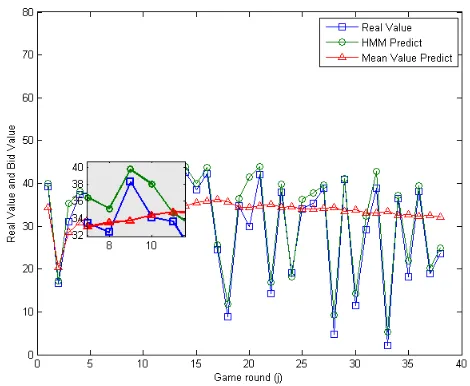
Figure 2. Comparison among real value, HMM prediction bids and Mean Value prediction bids
1) Comparison between prediction models: After the
training of data, the maximum bid value is limited to 20. And the amount of resources is set randomly in [0,100]. After 40 rounds of auctions, from Figure 2, we can envisage the comparison between the actual bids and prediction bids. It is obvious that the trend of HMM prediction bids approximates the actual bids most of the time. However, the mean value prediction [2] bids fluctuate without any connection with the actual bids. Thus, we can conclude from the results that the prediction model based on HMM can approximate the actual bids better than the prediction method adopted by [2].
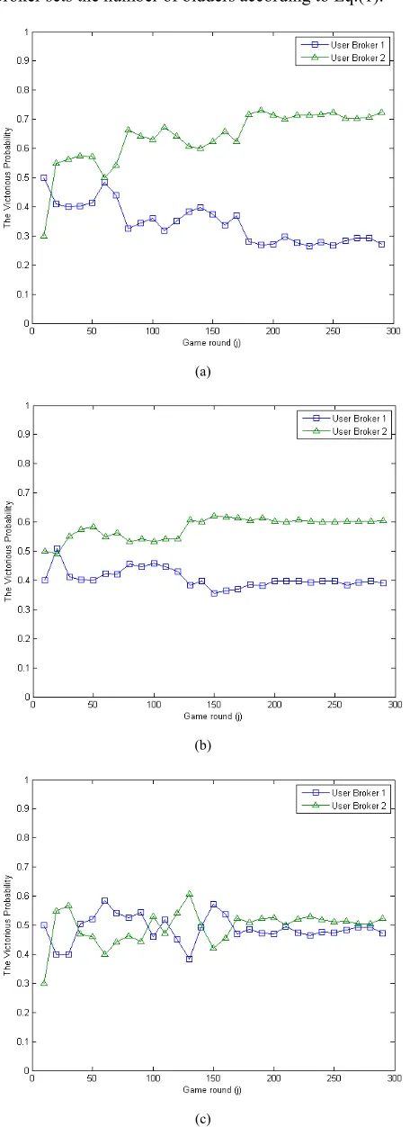
2) Victorious probability results of a two-player game.
Suppose that two user brokers (UB1 and UB2 ) are competing in the game. Specifically, if UB1 adopts no
prediction algorithm and UB2 utilizes the HMM prediction method, the results after 300 rounds of auctions are shown in Figure 3. It can be seen from Figure 3(a) that UB2 can achieve a higher victorious probability.
If UB1 adopts the mean value prediction method, and
2
UB still uses the HMM prediction method, the results is
depicted in Figure 3(b). It is apparent that UB2 ’s victorious probability still exceeds the UB1’s.
3) Victorious probability results of a multi-player game. On the analogy of the results of the two-player
Thus, to avoid this problem, our algorithm of resource broker sets the number of bidders according to Eq.(1).
(a)
(b)
(c)
Figure 3. Victorious probabilities comparisons.(a) Random bidding vs. ESPSA model (b) Mean value prediction model vs. ESPSA model (c)
ESPSA model vs. ESPSA model
Specifically, In ESPSA model, the method that we propose classifies the Sbidder into urgent set
u bidder
S and the
less urgent set v bidder
S . Then, according to each set, we
propose two different rounds of auctions. The number of bidders in each round should be calculated by Eq.(1). So the resource broker limits the number of user brokers in each auction by this way and guarantees the high victorious probability.
In order to prove the superiority of the ESPSA algorithms with user broker number restrictions, we made a comparison among actual victorious probability, expected victorious probability under user broker number restrictions and expected victorious probability without user broker number restrictions. The comparison results are depicted as Fig.4. For easy reference, we use ESPSA-NNres to represent the ESPSA algorithms without user broker number restrictions. It can be seen from Figure.4 that the difference between expected victorious probability and actual victorious probability is much smaller in the ESPSA algorithm. In the 10th round of the
auction, the average expected victorious probability is 0.4 and the result by ESPSA algorithm is 0.38. However, the ESPSA-NNres algorithm only gets a victorious probability of 0.34. Moreover, in the 30th round, user
brokers’ expected victorious probability is 0.58, the ESPSA’s and ESPSA-NNres’s victorious probabilities are 0.5 and 0.18 respectively.
Figure 4. Comparison between expected and actual victorious probability
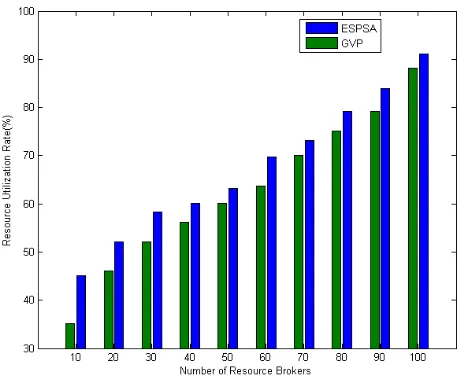
4) Resource utilization rate and execution time. By
Figure 5. Resource Utilization Rate of ESPSA and GVP
From Figure 6, the algorithm execution time comparison between GVP and ESPSA algorithm is illustrated. It is obvious that the ESPSA algorithm runs more quickly at the most of circumstances.
Figure 6. Algorithm execution time of ESPSA and GVP
Thus, according to the above analysis, we can see that the ESPSA model has higher superiority than GVP.
D. Equilibrium Analysis
Reference [2] utilized a mean value prediction method. Specifically, a player calculates his rival’s bid in the current round of auction by Eq.(8),
1
1 1
1
j
j i
i
b b
j −
=
=
−
∑
(8)Then, the player only needs to bid a litter higher than the prediction bid.
We adopt the Cobb-Douglas production function to calculate the actual value (As Eq.(9) shows).
(
, ,)
(
(
1)
ln ln)
v T Rα =η −α T+α R (9)
T represents the expected time that the user want to
hold the resource. R represents the amount of resources
that users want to have. α is a weighted factor which represents the preference of T and R. η is the profit
that brought by the unit payoff. In the experiment, we set
20
η= and α =0.95. Given one user broker’s historical resource demand quantities, through Eq.(9), the actual bid can be carried out.
By Eq.(8) and Eq.(9), the results are shown in Figure.2. The ESPSA algorithm performs better than the algorithm in [2] in approximating the actual value.
Figure.3 depicts the victorious probability results of random bidding, mean value prediction bidding and ESPSA prediction bidding strategies. Thus, the payoff matrixes can be given as follows.
Figure 7. Payoff matrix 1 of a two-user game
Figure 8. Payoff matrix 2 of a two-user game
From Figure 7 and Figure 8, it is obvious that the strict dominant strategy of user brokers is the ESPSA prediction strategy.
In a game, if a rational user agent has a strict dominant strategy, it will choose that strategy. In such way, the game reaches Nash equilibrium. For the reason that strict dominant strategy equilibrium must be Nash equilibrium [2], the two-player game above has Nash equilibrium:
(
)
* ESPSA Strategy , ESPSA Strategy S =
From the above analysis, we can conclude that the ESPSA predict strategy is superior to not only random bidding strategy but also mean value prediction strategy. Thus, all the rational players will choose the ESPSA strategy in the auction.
E. Computational Complexity of ESPSA
The Viterbi Algorithm provides a computationally efficient way of analyzing observation of HMMs to recapture the most likely underlying state sequence [26]. It exploits recursion to reduce computational complexity and takes advantage of the context of the whole sequence to make judgments. In conclusion, using the Viterbi algorithm to decode an observation sequence (the resource demand quantities), the computational load will only be linear in T [26].
Thus, we can get that any users who participate the game using the ESPSA model will acquire the grid or cloud resources with high victorious probability within a very short time.
F. Proof of Nash Equilibrium in ESPSA 1) Nash Equilibrium of a Two-user Game
In this paper’s setting, the users evaluate the value of an item according to the resource’s load information. If we assume that each resource’s load variation l is a
normal distribution, the payoff function of each user can be given by Eq.(10).
(
1)
11 , 1 , , , ; , 0, i i i m i
i i m i m
i
i
b if b wins
l
u b b b l b if b b
l m
if b loses
γ γ = ⎧ − ⎪ ⎪ ⎛ ⎞ ⎪ ⎛ ⎞ =⎨ ⎜ ⎜⎝ − ⎟⎠⎟ = = ⎝ ⎠ ⎪ ⎪ ⎪⎩
∑
(10) where γi is a constant, m is the total number ofparticipants in the game, bi is the bid price that user i
competes for a resource, and i=1, 2, ,… m. It is common
a same load may bring different benefit for different users, so the constant γi varies according to each user’s
profile. L is the load vector.
Without loss of generality, initially, a game, in which two users (that is m=2) compete for one resource, is
considered in the proof of Nash Equilibrium. Suppose that the strategies set of the users is
{
B B1, 2}
, and eachuser’s bidding function is strictly increasing. If given user 1’s bid, user 2’s payoff function is
(
)
2
2 2 1
2 2
2 1 2 2 1 2
1 2 1 , 1 , ; , 2 0, i
b if b b
l
u b b l l b if b b
if b b
γ
γ
=
⎧ − > ⎪ ⎪ ⎛ ⎞ ⎪ ⎛ ⎞ =⎨ ⎜ ⎜⎝ − ⎟⎠⎟ = ⎝ ⎠ ⎪ ⎪ < ⎪⎩
∑
(11)To prove the existence of Nash Equilibrium, firstly, user 2’s best response function need to be derived if given user 1’s bid.
Lemma 1. Given user 1’s bid strategy b1∈B1, user 2’s
best response is
( )
22 2
b l c
l γ
= .
Proof. Suppose that user 2’s probability density function is f
( )
γl (for the ease of proof, we suppose ii l
γ
η = ,
1, 2
i= ), user 2’s winning probability is
( )
(
( )
)
( )
(
)
( )
1
2 1 1
1
1 1
1 1
win
b
P b P b b
P b b
f d η η η η η − ≤ = ≤ = ≤ =
∫
(12)where 1 1
b− is the reverse function of user 1’s biding
function. In order to win, user 2 has to find a optimal strategy in strategy set B2 . So, this problem can be modeled by a non-linear programming problem represented by Eq.(13).
( )
(
( )
)
( ) ( ) ( )
2
1
2 2 2 2 2 2 2
1 1 2 2 1 1 2 2
max
. .
win b
b
f P b d
s t
b f f d d
η η η η η η η η η η α ≤ ≤
∫
∫ ∫
(13)where α2represents the budget of user broker 2 in a round of one auction.
It can be solved by a Lagrange multiplier. Then, we get Eq.(14).
( ) ( )
( ) ( ) ( )
(
)
( )
(
)
( )
( )
1 1 12 2 2 1 1 2
2 1 1 2 2 1 1 2 2
2 2 1 1 1 1 1 2 2 2
b
b
b
f f d d
b f f d d
b f d f d
η η η η η η η η λ η η η η η α η λ η η η η η ≤ ≤ ≤ − − ⎡ ⎤ = ⎢ − ⋅ ⎥⋅ ⎣ ⎦
∫ ∫
∫∫
∫ ∫
(14)It is obvious that, if the Eq.(14) gets maximum value, the objective of Eq.(13) gets its optimal value. Therefore, when η2−λ2⋅b1
( )
η1 =0 , the maximum value can beachieved. So, 2
2 opt
b =η λ . From 2
2 l
γ
η = , we get
2 2 opt b l γ λ
= . Suppose 2
2 1
c = λ , it is easy to get
( )
22 2
b l =c γ l . ■
Given user 2’s best response, the existence of Nash Equilibrium can be derived.
Theorem 1. In the ESPSA scheduling model with two
users, there exists Nash Equilibrium.
Proof: According to the Nash Existence Theorem [10, 11, 12], if each user’s strategy space is non-empty, closed and bounded convex set in Euler space and the payoff function is continuous, quasi concave function, there exists a pure Nash Equilibrium.
From the assumptions of ESPSA model, the strategy sets B1 and B2 are non-empty, closed and bounded. According to Eq.(10), the payoff function is continuous in its domain. From Lemma 1, it is obvious that the best
response,
( )
22
b l =c γ l , is convex under its domain.
Thus, payoff function is quasi concave [13]. ■ From the above prove, Nash Equilibrium exists in ESPSA model of two users.
2) Nash Equilibrium of N-winners Game
more realistic grid or cloud scheduling scenario setting is that multiple winners are allowed in one auction. It is because one resource always consists of several machines. Thus, in this section, we give a definition of the n-winner game and then propose a similar method of proving the Nash Equilibrium existence of a game.
Given user broker i’s bidding strategy bi∈Bi and the
strategy of user brokers except user broker UBi is
i i
b− ∈B− , i=1, 2, ,… m. User brokers aim to maximize
their own expected benefit, while satisfying their budgets. Thus, the payoff function of user broker i can be written as Eq.(15).
(
)
(
)
(
)
1 2
1 2
, max , , , , ;
0, max , , , i
i i n m
i i i
i n m
b b b b b
l
u b b l
b b b b
γ − ⎧ − ∈ ⎪ = ⎨ ⎪ ∉ ⎩ … … (15) where n is the number of winners, and we use
(
1 2)
maxn b b, , ,… bm , 0< ≤n m, to represent the top n
bids in
{
b b1, , ,2 … bm}
.Lemma 2. Given the payoff function of each user broker
and the bidding strategy of other user brokersb−i, in the
n-winners ESPSA game, the best bidding strategy of a user broker i is in the form of i
i
b c
l γ
= , where c is a
constant.
Proof: The strategies for user broker i can be represented
as the set of bidding functionsBi =
{
b b b1, ,2 3 bm}
. Inorder to prove the existence of Nash Equilibrium, the form of response correspondence of each user broker
( )
b ⋅ has to be derived.
Given all the other user brokers’ (except user broker i)
bid b−i, the expected payoff of user broker i is:
(
)
(
1 2)
Pr max , , ,
i
i i i n m
u b b b b b
l
γ
=⎡⎢ − ⎤⎥⋅ ∈
⎣ ⎦ … (16)
where Pr
(
bi∈maxn(
b b1, , ,2 … bm)
)
is the probability ofi
b in the set of top n bids. i i b l γ − ⎛ ⎞ ⎜ ⎟
⎝ ⎠ represents the net
payoff of UBi when it wins the game. Let ωn be the set
of winners, and i
n
ω
− be the n winners without the
participation of UBi. It is obvious that the bid of UBi
only needs to be greater than the least one in the set i
n
ω
− .
Thus, we use ( ) i
Least
b ω
− to represent that user broker. Thus,
to win the game, user broker i’s bid only need to be greater than ( )
i
Least
b ω
− . For the sake of simplicity, that user
broker is represented by UBL and its bid as bL. Thus,
i
UB ’s optimal bidding function can be represented by
(
)
{
2}
max Pr
. . Pr
i
i i L i
bi
L L i
u b b b
l
s t
b b b w
γ
⎡ ⎤
=⎢ − ⎥⋅ < ⎣ ⎦
⋅ < ≤
(17)
ESPSA is an extended version of second sealed price sealed auction. It allows multiple winners and the payment of a winner k is the least winner’s bid without
the participation of the user brokerk. Then, the payment
of user broker i is bL as the constraint term of Eq. (17)
shows.
By applying the similar method, we can derive the result. The analysis is omitted for briefness. ■
Theorem 2: A Nash Equilibrium exists in the ESPSA
game G=⎣⎡m S,
{ }
i ,{ }
ui( )
⋅ ⎤⎦ with{ }
Si and ui( )
⋅ defined above.Proof: The proof can follow the steps of Theorem 1 to show the existence of Nash equilibrium. For the sake of briefness, we omitted them here. ■
V. CONCLUSION AND FUTURE WORK
The ESPSA model is proposed in this paper and the model focuses on the resource allocation problem in grids and cloud computing. Firstly, we designed the interactions procedures between different entities in the ESPSA. Then, the algorithms of user and resource brokers are proposed. Specifically, in order to assure the victorious probability of each user broker, we introduce a bidder number restriction method in the resource broker’s algorithm. Moreover, the user broker gets prediction information from the analyst who adopts the HMM prediction model. Then, based on the prediction results, the user broker carries out its bid. Simulation results show that, the ESPSA algorithms bids performs better in the approximation to actual bids than random bidding and mean value predict strategy. What’s more, we analyzed the existence of Nash equilibrium based on the simulation results and the computational load of the ESPSA model. Lastly, we proved the existence of Nash equilibrium of the ESPSA model with two participants and multi- participant theoretically.
It is worthwhile to note that the ESPSA model is much more applicable than some basic auction models. However, the network delay, fraud user, reliability of resources problems are not considered in this paper. Thus, how to make the model realistic, fulfill the QoS requirements of users and improve the resource scheduling algorithms form the next step of our work.
ACKNOWLEDGMENT
This paper is partially supported by NSFC-JST under grant No.:51021140004; Nature Science Foundation of China under grant No.: 60673046, 90715037; University Doctor Subject Fund of Education ministry of China under grant No.: 200801410028; National 973 Plan of China under grant No.: 2007CB714205; Natural Science Foundation Project of Chongqing, CSTC under grant No.: 2007BA2024; Natural Science Foundation of China under Grant No. 60903153; the Fundamental Research Funds for the Central Universities; Nature Science Foundation of China under grant No.61070181.
[1] Qiufen Xia, Weifeng Sun, Zichuan Xu, Mingchu Li, “A Novel Grid Resource Scheduling Model Based on Extended Second Price Sealed Auction”, 3rd International Symposium on Parallel Architectures, Algorithms and Programming, Dalian, pp. 305-310, 2010.
[2] Lei Yao, Guanzhong Dai, Huixiang Zhang, Shuai Ren, and
Yun Niu, “A novel algorithm for task scheduling in grid computing based on game theory”, The 10th IEEE International Conference on High Performance Computing and Communications, pp. 282-287, 2008.
[3] Maheswaran, R.T., and Basar, T., “Nash equilibrium and
decentralized negotiation in auctioning divisible resources”, Group Decision and Negotiation, pp. 361–395, 2003.
[4] Kwok, Y.K., Song, S.S. and Hwang, K., “Selfish grid
computing: Game-theoretic modeling and NAS performance results”, In Proceedings of CCGrid, pp. 349– 356, 2005.
[5] Bredin J., Kotz D., Rus D., Maheswaran R.T., Imer C., and
Basar T., “Computational markets to regulate mobile-agent systems”, Autonomous Agents and Multi-Agent Systems, pp. 235–263, 2003.
[6] LI Zhijie, Cheng Chuntian, Huang Xuefei, and Li Xin, “A
sequential game-based resource allocation strategy in grid environment”, Journal of Software, pp. 2373-2383, 2006. (in Chinese with English abstract).
[7] Abramson D., Buyya R., and Giddy J., “A computational
economy for grid computing and its implementation in the nimrod-G resource broker”, Future Generation Computer Systems, pp. 1061−1074, 2002.
[8] Amazon Elastic Compute Cloud(EC2).
http://aws.amazon.com/ec2.
[9] Microsoft Azure Services Platform.
http://www.microsoft.com/azure/default. mspx.
[10] Rackspace Mosso. http://www.mosso.com/.
[11] Ristenpart, T., Tromer, E., Shacham, H., and Savage, S..
“Hey, you, get off of my cloud: exploring information leakage in third-party compute clouds”, In Proceedings of the 16th ACM Conference on Computer and Communications Security, New York, pp. 199-212, 2009.
[12] Chonho Lee, Junichi Suzuki, Athanasios Vasilakos, Yuji
Yamamoto, and Katsuya Oba., “An evolutionary game theoretic approach to adaptive and stable application deployment in clouds”, In Proceeding of the 2nd workshop on bio-inspired algorithms for distributed systems, ACM, New York, pp. 29-38, 2010.
[13] Guiyi Wei, Athanasios Vasilakos, Yao Zheng and Naixue
Xiong, “A game-theoretic method of fair resource allocation for cloud computing services”, The Journal of Supercomputing, vol. 54, p. 252-269,2010.
[14] Rajkumar Buyya and Manzur Murshed, “GridSim: a
toolkit for the modeling and simulation of distributed resource management and scheduling for Grid computing”, Concurrency and Computation: Practice and Experience, pp. 1175-1220, 2002.
[15] Fei Teng and Frédéric Magoulès, “A New Game
Theoretical Resource Allocation Algorithm for Cloud Computing”, Advances in Grid and Pervasive Computing, pp. 321-330, 2010.
[16] Korilis. Y.A., Varvarigou. T.A. and Ahuja. S.R.,
"Incentive-compatible pricing strategies in non-cooperative networks", Seventeenth Annual Joint Conference of the IEEE Computer and Communications Societies, vol. 2, pp. 439-446, 29 Mar-2 Apr 1998.
[17] Marbach, P., "Pricing differentiated services networks:
bursty traffic”, Twentieth Annual Joint Conference of the
IEEE Computer and Communications Societies, vol. 2, pp. 650-658, 2001.
[18] Ranganathan. K., Ripeanu. M., Sarin. A. and Foster. I.,
"Incentive mechanisms for large collaborative resource sharing", Cluster Computing and the Grid, pp. 1- 8, April 2004.
[19] D.E. Volper, J.C. Oh and M. Jung, “GameMosix:
Game-theoretic middleware for CPU sharing in untrusted P2P eEnvironment”, Parallel and Distributed Computing and Systems (SPDCS), 2004.
[20] Micah Adler, Rakesh Kumar, Keith Ross, Dan Rubenstein,
David Turner, and David D. Yao. “Optimal peer selection in a free-market peer-resource economy”, In Proceedings of the Second Workshop on Economics of Peer-to-Peer Systems, 2004.
[21] Luzi Anderegg and Stephan Eidenbenz, “Ad hoc-VCG: a
truthful and cost-efficient routing protocol for mobile ad hoc networks with selfish agents”, In Proceedings of the 9th annual international conference on Mobile computing and networking (MobiCom '03), New York, pp. 245-259, 2003.
[22] Milgrom and Paul, "Auctions and Bidding: A Primer",
Journal of Economic Perspectives, American Economic Association, pp. 3-22, 1989.
[23] Buyya R., Abramson D. and Giddy J., “A case for
economy grid architecture for service-oriented grid computing”, In: Proceedings of the 10th IEEE Int’l Heterogeneous Computing Workshop, IEEE Computer Society, Washington, pp. 776−790, 2001.
[24] Guiyi Wei, Vasilakos. A.V. and Naixue Xiong,
"Scheduling parallel cloud computing services: an evolutional game", 1st International Conference on Information Science and Engineering, pp. 376-379, December 2009.
[25] Durbin R, Eddy S, Krogh A and Mitchison G, “Biological
sequence analysis: Probabilistic models of proteins and nucleic acids”, Cambridge, in Cambridge University Press, 1998.
[26] http://www.comp.leeds.ac.uk/roger/HiddenMarkovModels/
html_dev/main.html
Weifeng Sun is an assistant professor in
software school at the Dalian University of Technology(DLUT). Most of his research centers around high quality wireless communictions on wireless multihop network(such as WMN,WSN,MIPv6 and so on) and scheduling and applications on distributed network(including Grid Computing and Cloud Computing). He got the PH.D degree and bachelor degree at University of Science and Technology of China(USTC).Additional information about Sven can be found on his webpages:home.ustc.edu.cn/~wfsun.
Qiufen Xia, born in 1987, received the M.A. from Dalian
University of Technology, Dalian in 2009. She is a master student of software school, Dalian University of Technology. Her study interests include grid resources scheduling, game theory, network security and cloud computing.
Zichuan Xu, born in 1986, male, received Master degree and
Technology, China. His research interests include approximation algorithms, temperature-aware scheduling, cyber-physical systems (CPS), game theory, green computing.
Mingchu Li received the B.S. degree in mathematics, Jiangxi
Normal University and the M.S. degree in applied science , University of Science and Technology in 1983 and 1989, respectively. He worked for University of Science and Technology in the capacity of associate professor from 1989 to 1994. He received his doctorate in Mathematics, University of Toronto in 1997. He was engaged in research and development on information security at Longview Solution Inc, Compuware Inc. from 1997 to 2002. From 2002, he worked for School of
Software of Tianjin University as a full professor, and from 2004 to now, he worked for School of Software of Dalian University of Technology as a full Professor, Ph.D. supervise, vice dean. His main research interests include theoretical computer science and cryptography.
Zhenquan Qin received the bachelor degree in security