COMPRESSIVE SENSING BASED IMAGE RECONSTRUCTION

Sherin et al. World Journal of Engineering Research and Technology

COMPRESSIVE SENSING BASED IMAGE RECONSTRUCTION

Sherin C. Abraham1* and Ketki Pathak2

1

Electronics and Communication department, Dr. S and S. S Ghandhy College of

Engineering and Technology, Majura Gate, Surat, India.

2

Electronics and Communication department, Sarvajanik College of Engineering and

Technology, Surat, India.

Article Received on 04/03/2017 Article Revised 25/03/2017 Article Accepted on 14/04/2017

ABSTRACT

Compressive sensing is a technique of image acquisition and

reconstruction from a relatively fewer measurements than what the

Nyquist theorem suggests; the sampling rate must be greater than twice

the highest frequency in the signal for fidelity of image reconstruction.

Compressive sensing is applicable when the signals under

consideration are sparse. Two-dimensional discrete wavelet transform

is applied for sparse representation of an image in this thesis. When

sparsity is more, the performance of compressive sensing image reconstruction algorithm will

be better. The sparse level of low frequency sub bands and high frequency sub bands are

different. Two different compressive sensing measurement matrixes and recovery algorithms

are used for the low-frequency sub bands and high-frequency sub bands for better results.

Medical field especially in MRI scanning, compressive sensing can be utilized for less

scanning time, thus benefits patients. The reconstructed image will be better in both PSNR

and visual quality.

KEYWORDS: Compressive Sensing, Wavelet Transform, Discrete Cosine Transform, Sparsity, MRI.

INTRODUCTION

We are in the midst of a digital revolution that is driving the development and deployment of *Corresponding Author

Sherin C. Abraham

Electronics and

Communication department,

Dr. S and S. S Ghandhy

College of Engineering and

Technology, Majura Gate,

Surat, India.

World Journal of Engineering Research and Technology

WJERT

videos, and other data can be exactly recovered from a set of uniformly spaced samples taken

at the so-called Nyquist rate. Unfortunately, in many important and emerging applications,

the resulting Nyquist rate is so high that will end up with far too many samples. Alternatively,

it may simply be too costly, or even physically impossible, to build devices capable of

acquiring samples.

A new technology is required in this world where we are using HD videos, video

conferencing, online games, etc. much more than ever. Now we have a solution, Compressive

Sensing. The signal having a sparse representation can be recovered exactly from a small set

of linear, non-adaptive measurements. It means it‟s possible to sense sparse signals by taking

far fewer measurements, lower sampling rate, hence the name compressed sensing.

CS differs from classical sampling in three important respects. First, CS is a mathematical

theory focused on measuring finite-dimensional vectors in RN. Second, CS systems typically

acquire measurements in the form of inner products between the signal and more general test

functions. Thirdly, the signal recovery is typically achieved using highly nonlinear methods.

In short, CS enables a potentially large reduction in the sampling and computation costs for

sensing signals that have a sparse or compressible representation.

Nomenclature

CS Compressive Sensing

WT Wavelet Transform

DCT Discrete Cosine Transform

OMP Orthogonal Matching Pursuit

DWT Discrete Wavelet Transform

HD High Definition

i.i.d identically and independent dependent

MRI Magnetic Resonance Imaging

MSE Mean Square Error

PSNR Pseudo SNR

In this paper we applied CS in the medical images and analyzed using different sparsity

domain, measurement matrix and reconstruction algorithm. WT and DCT are used as sparsity

domain. Hadamard matrix and Gaussian matrix are considered as measurement matrix. L1

minimization, Orthogonal Matching Pursuit and pseudo inverse multiplication method are

used as recovery algorithm.

Applications

where it has enabled speedups by a factor of seven in paediatric MRI while preserving

diagnostic quality.

Basic Concept of Medical Imaging

CS is being actively pursued for medical imaging, particularly in MRI. Most MR images, like

angiograms, have sparsity properties, in domains such as Fourier or wavelet basis. Generally,

MRI is a costly and time consuming process because of its data collection process which is

dependent upon physical and physiological constraints. In addition, high gradient amplitudes

and rapid switching can produce peripheral nerve stimulation. However, the introduction of

CS based techniques has improved the image quality through reduction in the number of

collected measurements and by taking advantage of their sparsity, thus benefits patients.

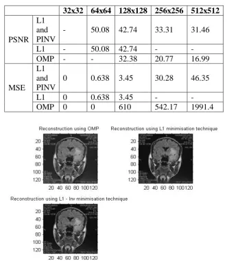
Figure 1: MRI image reconstructed using various techniques.[6] Compressive Sensing – Basic Introduction

Basic Block Diagram of CS based system

The recent theory of Compressive Sensing introduced by Candes, Romberg, and Tao and

Donoho demonstrates that a signal that is K-sparse in one basis (call it the sparsity basis) can

be recovered from cK non-adaptive linear projections onto a second basis (call it the

measurement basis) that is incoherent with the first, where c is a small over-measuring

constant. While the measurement process is linear, the reconstruction process is decidedly

nonlinear.

Let x is a real valued, finite length, one dimensional, discrete time signal which is an Nx1

Figure 2: Block diagram of compressive sensing.[1] Thus signal x can be written as

x = Ψ f

 f is Nx1 column vector of weighting coefficients f= = ΨT x

 f is the sparse representation of signal x in the orthonormal basis Ψ.

The signal x is K-sparse if it is a linear combination of only K nonzero basis vectors. When K

<< N, the signal x is compressible, means it has just a few large coefficients and many small

coefficients.

We measure the signal x by sampling it with respect to a measurement matrix Φ ∈ RMxN. The

measurement MxN matrix Ф must allow the reconstruction of the length-N signal x from M < N measurements. The measurement process is not adaptive, meaning that Ф is fixed and

independent of signal x. Thus measurements M×1 vector y can be represented:

y = ФΨf = Acsf = Фx

 Acs = ФΨ is the sensing matrix of M x N.

 Ф is the measurement matrix.

 Ψ and Ф should be incoherent.[1]

x

y

X

Figure 3: Sparsity and incoherence in wavelet transform enables the megapixel image to its approximation obtained by throwing away 97.5% of the coefficients with negligible perceptual loss. (a) Original Image (b) Wavelet transform coefficients (c) Reconstructed image.[10]

Reconstruction Algorithms Linear Optimisation

To recover the signal by L1-norm minimization; the reconstruction x* is given by x* = Ψf*,

where f* is the solution to the convex optimization program

(||f|| l1 := ) l1 subject to yk = , ∀ k ∈ M

That is, among all objects = Ψ consistent with the data, pick only whose coefficient

sequence has minimal L1 norm. The CS theory uses L1 norm characteristics which are linear

in nature and can be easily computed, thus offering a far simpler and faster way of estimating

sparse signals from very limited number of measurements.

Greedy algorithm uses an iterative approach of the coefficient signal to the signal

convergence is reached, or get an approximate increase of sparse signal in each of iteration by

calculating the measured data mismatch. OMP is one of greedy algorithms.[7]

Proposed Algorithm

The proposed algorithm is given in fig 4. The image is undergone two - dimensional wavelet

transform for more sparsity. In the image reconstruction based on the traditional compressive

sensing algorithm, the same measurement matrix is used to measure the whole wavelet

coefficients. However, since the high-frequency coefficients are sparse while the low

frequency coefficients are not sparse,[2] when putting the low frequency coefficients together

with the high-frequency coefficients to multiply with the measurement matrix, the coherences

performance of the reconstructed image.[3] The scaling coefficients of low-frequency

component contain most of the image energy.

Due to these DWT features, two random CS sensing matrices are separately used for

re-sampling the low-band and high-bands, which can be expressed as follows:

where YL and YH denote CS samples measured from low-bands and high-bands, while XL

and XH represent the scaling and wavelet coefficients, respectively. At the decoder side, two

different CS recovery algorithms are developed for the low-frequency subband and

high-frequency subbands, respectively.

The required number of CS measurements is much smaller than that of the DWT coefficients,

and therefore, CS sampling. The challenge is to get the reconstructed image in better quality

by adding more sparsity with maintaining incoherence. For this, we need to choose

measurement matrix and recovery algorithm wisely.

Implementation

Algorithm Steps For Implemenation The steps of the algorithms are as follows:

(1) Perform the wavelet transform of the N*N image, and get the four wavelet sub-band

coefficients {LH1, HL1, HH1, LL1}.

(2) Use the measurement matrix to measure the three high-frequency sub-band coefficients

LH1, HL1, HH1 to get the matrices of the measured coefficients while use another

measurement matrix for the low-frequency sub-band coefficients LL1.

(3) Use the reconstruction algorithms to reconstruct the three high-frequency coefficients

matrices 1, 1, 1, and low-frequency coefficients matrix LL1. Then together

reconstruct the image.

(4) The image reconstructed will be verified by its PSNR value.

Simulation setup

The scaling coefficients XL are re-sampled by an i.i.d. random Hadamard matrix ΦL. The

scaling coefficients XH are re-sampled by an i.i.d. random Gaussian matrix ΦH. L1

minimization technique, OMP and Pseudo Inverse multiplication method reconstruction

techniques are used as reconstruction algorithms.

We have used different size of images like 32x32, 64x64, 128x128 and 512x512. The

transform method DCT is also compared with wavelet transform.

Results of implementation of proposed block diagram.

Figure 5: Wavelet Transform Output of 128x128 image.

Figure 6: Wavelet coefficients of 128x128 image before measurements taken.

Figure 7: Wavelet coefficients of 128x128 image after measurements taken.

CS makes the signal sparser, which is clear by comparing the Fig.6 and Fig.7. This sparsity

leads to the efficient lossless compression. Due to more sparsity, the reconstructed image

quality will be more.

The outputs of different images are compared based on PSNR and MSE values with iteration

value 50. The images are undergone WT.

Table 1: MSE and PSNR values comparison for different medical images for 50 iteration. Medical image 1 Medical image 2 Medical image 3 Medical image 4 PSNR L1 and PINV

43.83 54.85 31.76 30.11

OMP 15.28 18.21 19.77 14.23

MSE L1 and PINV

2.699 .212 43.27 63.36

OMP 1971.3 981 684.86 2455

The outputs of different image sizes are compared based on PSNR and MSE values with

iteration value 50. The image has undergone WT.

Table 2: MSE and PSNR values using L1 minimization or OMP with different sizes of images.

32x32 64x64 128x128 256x256 512x512

PSNR L1 and PINV

- 50.08 42.74 33.31 31.46

L1 - 50.08 42.74 - -

OMP - - 32.38 20.77 16.99

MSE L1 and PINV

0 0.638 3.45 30.28 46.35

L1 0 0.638 3.45 - -

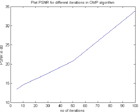
Table 3: PSNR comparison for various number of iterations. Iterations

PSNR using 32x32

PSNR using 64x64

PSNR using 128x128

PSNR using 256x256

PSNR using 512x512

5 17.87 15.76 14.53 13.5 12.96

10 23.37 18.57 15.86 14.6 13.66

15 36.67 21.08 17.25 15.34 14.14

25 - 30.39 20.25 16.84 15.1

50 - - 30.39 20.77 16.99

100 - - - 33.88 21.12

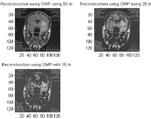
The PSNR is compared with different number of iterations using OMP reconstruction

algorithm.

Figure 10: Output of 128x128 image using different iterations of OMP.

PSNR values for different size of images respectively are plotted in fig 10. As size increases

the PSNR values is getting decreased. But as size decreases the details of the image will get

lost. As numbers of iterations are increasing, the image quality is also increasing as shown in

fig 11. From table II we can conclude that less size and more iteration will result in better

image.

Figure 12: PSNR for different iterations in OMP reconstruction algorithm. The wavelet transform is compared with DCT. The image undergone DCT, and

measurements are taken using Hadamard matrix and without packet loss in the channel.

When size increases, the quality will be reducing. OMP with 50 iterations is used.

Table 4: MSE and PSNR comparison using DCT with Hadamard Matrix. 32x32 64x64 128x128 256x256 512x512

PSNR OMP - 50.18 38.59 28.55 27.14

MSE OMP 0 0.546 9.1443 90.73 122.4

Table 5: MSE and PSNR comparison using DCT with Gaussian Matrix. 32x32 64x64 128x128 256x256 512x512 PSNR

PINV 19.9 19.45 19.06 18.04 18.02

L1 36.13 28.45 26.02 22.24 20.35

OMP - 36.14 32.5 25.94 25.37

MSE

PINV 665.4 774.4 805.9 1013.5 1023.5

L1 15.84 98.85 163.45 388.9 520.3

OMP 0 15.16 36.56 165.4 188.6

OMP is better than L1 and PINV methods when Gaussian matrix is used as measurement

Inferences

 When size of image increases, the PSNR value decreases.

 For small size images, OMP reconstruction is better. And for large size images, L1

minimization output is better.

 PSNR will increase when number of iterations is increased for OMP reconstruction

algorithm.

 Hadamard matrix is better than Gaussian matrix when use after DCT.

 Wavelet transform is better when OMP reconstruction algorithm is used.

 Due to the sparsity in the signal, the required compression is achieved.

CONCLUSION

The Compressive sensing measures a relatively small number of “random” linear

combinations of the signal value. Sparsity, incoherence and nonlinear reconstruction are three

main components of CS. The sparse nature of signals in a particular basis by taking

measurements in an „incoherent‟ basis is utilized in CS.

Wavelet transform is proven sparsity domain for many signals. The high-frequency

coefficients are sparse while the low frequency coefficients are not sparse. So, both should be

processed separately for better results. But in DCT transform, we cannot separate the

components on basis of frequency. Hadamard measurement matrix is better. L1 minimisation

is better with wavelet transform and OMP will be better with DCT.

In Medical field, CS will help in less number of samples, less radiation for patients. The

medical images are inherently sparse and incoherence.

Future works possible

 Reduce the processing time using Block-based CS method.

 Add enough sparsity by sparsity tuning and intra-prediction methods.

ACKNOWLEDGEMENT

To all my friends and family who supported me to prepare this paper.

REFERENCE

1. Chenwei Deng, Weisi Lin, Bu-sung Lee, and Chiew Tong Lau, "Robust Image Coding

14(2).

2. Xiumeni Li and Guoan Bi, “Image reconstruction based on the improved compressive

sensing algorithm”, IEEE International Conference on Digital Signal Processing (DSP),

2015.

3. Weisheng Dong, Xiaolin Wu, and Guangming Shi, "Sparsity Fine Tuning in Wavelet

Domain with Application to Compressive Image Reconstruction”, IEEE Transactions on

Image Processing, December 2014; 23(12).

4. Muhammad Ali Qureshi and M. Deriche, “A new wavelet based efficient image

compression algorithm using compressive sensing”, Springer Science Multimedia tools

and applications, March 2015.

5. Michael Lustig and et.al, “Compressed sensing MRI”, IEEE signal processing magazine,

March, 2008.

6. Sabbisetti Ravindranath and et. al, “Compressive Sensing based Image acquisition and

Reconstruction analysis” Green Computing Communication and Electrical Engineering

(ICGCCEE), 2014 International Conference.

7. Chen Chen and Junzhou Huang, “Exploiting the wavelet structure in compressed sensing

MRI”, Science Direct Magnetic Resonance Imaging, July 2014.

8. Saad Qaisar and et.al, “Compressive sensing: From theory to applications, a survey”,

IEEE Journal of communications and networks, October 2013; 15(5).

9. Emmanuel J. Candès and Michael B. Wakin, “An introduction to compressive sensing”,

IEEE Signal Processing Magazine, March 2008.

10.S. Spurthi and Parnasree Chakraborty, “Block based compressed sensing algorithm for

medical image compression”, International Journal of Engineering and Computer

Science, May 2016; 05(5).

11.Sumit Budhiraja and Dipti Bhatnagar, “Wavelet based compressive sensing techniques

for image compression”, International journal of Engineering Research and Applications,

2011.

12.Dr. G Vijay Kumar, “Fast compressed sensing based high resolution image

reconstruction”, International Journal of New Technology and Research, March 2016;

2(3).

13.Jie Xu and et.al, “Improved total variation minimization method for compressive sensing

by intra-prediction”, Science direct, Signal processing, 2012.

Acoustics, Speech and Signal Processing, 2013.

15.Quisong Wu and et.al, “Multi-task Bayesian compressive sensing exploiting intra-task

dependency”, IEEE signal processing letters, 2013.

16.http://dsp.rice.edu/sites/dsp.rice.edu/files/cs/baraniukCSlecture07.pdf

17.http://dsp.rice.edu/cs

18.https://en.wikipedia.org/wiki/Compressed_sensing

19.Civil Hospital, Surat

20. https://www.ncm-c.org/services/diagnostic-imaging/magnetic-resonance-imaging-mri/