Improving the Student’s Performance Using
Educational Data Mining
K.Shanmuga Priya
Department of Computer Science, Hindusthan College of Arts & Science, Coimbatore-28 Email: [email protected]
A.V.Senthil Kumar
Director, Department of MCA, Hindusthan College, Coimbatore-28 Email: [email protected]
---ABSTRACT---
The main goal of educational data mining is to improve the student performance. The usage of data mining techniques which achieves the goal in an efficient manner. The discovery of knowledge that extract from the end semester [1] is one of the method for improving the quality of higher education. In the higher education, the analysis on enrolment of student’s performance in a particular course, the student talent, confidence, studies and ethic helps to get more knowledge. In this research, the data classification and decision tree [1] which helps to improve the student’s performance in a better way. But with the inclusion of extracurricular activities with the above data mining techniques makes quality of education in an easiest way. This type of approach gives high confidence to students in their studies. This method helps to identify the students who need special advising or counseling by the teacher which gives high quality of education.
Keywords – Classification, Educational Data Mining (EDM), ID3 Algorithm, Knowledge Discovery in Database (KDD)
‐‐‐‐‐‐‐‐‐‐‐‐‐‐‐‐‐‐‐‐‐‐‐‐‐‐‐‐‐‐‐‐‐‐‐‐‐‐‐‐‐‐‐‐‐‐‐‐‐‐‐‐‐‐‐‐‐‐‐‐‐‐‐‐‐‐‐‐‐‐‐‐‐‐‐‐‐‐‐‐‐‐‐‐‐‐‐‐‐‐‐‐‐‐‐‐‐‐‐‐‐‐‐‐‐‐‐‐‐‐‐‐‐‐‐‐‐‐‐‐‐‐‐‐‐‐‐‐‐‐‐‐‐‐‐‐‐‐
Date of Submission: January 11, 2013 Date of Acceptance: February 12, 2013
‐‐‐‐‐‐‐‐‐‐‐‐‐‐‐‐‐‐‐‐‐‐‐‐‐‐‐‐‐‐‐‐‐‐‐‐‐‐‐‐‐‐‐‐‐‐‐‐‐‐‐‐‐‐‐‐‐‐‐‐‐‐‐‐‐‐‐‐‐‐‐‐‐‐‐‐‐‐‐‐‐‐‐‐‐‐‐‐‐‐‐‐‐‐‐‐‐‐‐‐‐‐‐‐‐‐‐‐‐‐‐‐‐‐‐‐‐‐‐‐‐‐‐‐‐‐‐‐‐‐‐‐‐‐‐‐
1. Introduction
D
ata mining is the powerful technology for analyzing important information from the data warehouse. It is the extraction of hidden predictive information for better decision making. Data mining is one of the steps in KDD process. Knowledge discovery (KDD) aims at the discovery of useful information from large collections of data [2]. The main goal of data mining in the KDD process concerned with the algorithmic means by which patterns or structures are enumerated from the data under acceptable computational efficiency limitations. The new concept of educational data mining techniques, is rapidly growing [3] in the education field. It helps to make analysis on the student activities and also improves their performance.The scope of this research paper, makes to extract the knowledge discover from the student database for improving the student performance. Here by, data mining techniques such as data classification and decision tree methods are used to evaluate the student performance. The analysis of performance can be done in several ways such as Overall Semester Marks, Practical Lab, Attendance, Paper Presentation, End Semester Marks etc.,
1.1 Decision Tree
A Decision tree is a classification Scheme which generates a tree and set rules, representing the model of different classes, from a given data set. A decision tree can be used to clarify and find an answer to a complex problem. The structure allows users to take a problem with multiple possible solutions and display it in a simple, easy-to-understand format that shows the relationship between different events or decisions. The furthest branches on the tree represent possible end results.
There are three decision tree algorithms are used to make the decision efficiently. Those are ID3, ASSISTANT and C4.5.
2. Related Work
colleges of Dr.R.M.L. Awadh University, Faizabad, India. By means of Bayes Classification on Category, Language and background qualification, it was found that whether new comer students will performer or not.
Galit [5] gave a case study that use students data to analyze their learning behavior to predict the results and to warn students at risk before their final exams.
Bray [6], in his study on private tutoring and its implications, observed that the percentage of students receiving private tutoring in India was relatively higher than in Malaysia, Singapore, Japan, China and Sri Lanka. It was also observed that there was an enhancement of academic performance with the intensity of private tutoring and this variation of intensity of private tutoring depends on the collective factor namely socio-economic conditions.
Pandey and Pal [7] conducted study on the student performance based by selecting 60 students from a degree college of Dr. R. M. L. Awadh University, Faizabad, India. By means of association rule they find the interestingness of student in opting class teaching language.
Khan [8] conducted a performance study on 400 students comprising 200 boys and 200 girls selected from the senior secondary school of Aligarh Muslim University, Aligarh, India with a main objective to establish the prognostic value of different measures of cognition, personality and demographic variables for success at higher secondary level in science stream. The selection was based on cluster sampling technique in which the entire population of interest was divided into groups, or clusters, and a random sample of these clusters was selected for further analyses. It was found that girls with high socio-economic status had relatively higher academic achievement in science stream and boys with low socio-economic status had relatively higher academic achievement in general.
Han and Kamber [9] describes data mining software that allow the users to analyze data from different dimensions, categorize it and summarize the relationships which are identified during the mining process.
Ayesha, Mustafa, Sattar and Khan [10] describe the use of k-means clustering algorithm to predict student s learning activities. The information generated after the implementation of data mining technique may be helpful for instructor as well as for students.
Bhardwaj and Pal [11] conducted study on the student performance based by selecting 300 students from 5 different degree college conducting BCA (Bachelor of Computer Application) course of Dr. R. M. L. Awadh University, Faizabad, India. By means of Bayesian classification method on 17 attribute, it was found that the
factors like students grade in senior secondary exam, living location, medium of teaching, mother’s qualification, students other habit, family annual income and student s family status were highly correlated with the student academic performance.
Al-Radaideh, et al [12] applied a decision tree model to predict the final grade of students who studied the C++ course in Yarmouk University, Jordan in the year 2005. Three different classification methods namely ID3, C4.5, and the NaïveBayes were used. The outcome of their results indicated that Decision Tree model had better prediction than other models.
3. Proposed Work 3.1 ID3 Decision Tree
The ID3 algorithm was invented by Ross Quinlan. It is a precursor to the c4.5 algorithm. We can create the decision tree in a given data set using this ID3 algorithm. This algorithm classifies the data using attributes. ID 3 follows the Occams’s Razer Principle. It is used to create the smallest possible decision tree.
In an educational system student’s performance can be improved by analyzing the internal assessment and end semester examination. Internal assessment means class test, seminar, attendance, lab practical would be conducted by the teacher. Along with the internal assessment, communication skill and paper presentations done by the student in their academic days are also needed to analyze for the improvement of student’s performance.
3.2 Data set
The data set used is obtained from M.Sc IT department of Information Technology 2009 to 2012 batch, Hindustan College of Arts and Science, Coimbatore. First 50 student’s data is taken as sample and errors were removed.
Some of the fields were selected which are required for data mining process. Some derived attributes were included. These attributes are given in Table – I.
Table – I. Selected Attributes for data set.
Attributes Description Possible Values
OSM Overall Semester Marks
{ First >59%, Second >49% &<60%
Third >34% & <39%
CT Class Test {Good, Average, Poor}
SEM Seminar
Performance {Good, Average, Poor} CS Communication
Skill
{Good, Average, Poor}
PP Paper
Presentations {Yes, No}
ATT Attendance {Good, Average,
Poor} PL Practical Lab {Yes, No}
ESM End semester
Marks { First >59%, Second >49% &<60%
Third >34% & <39%
Fail <40%
The values for the attributes are explained as follows for the current analysis.
SM – Overall Semester Marks are obtained from M.Sc IT. It is divided into four values: First >59%, Second >49% and <60%, Third >34% and < 39%, Fail < 40%.
2. CT – Class Test is obtained. In each semester two class tests are conducted. It is split into three classes: Good – 60%, Average >39% and < 60% and Poor < 40%.
3. SEM – Seminar Performance is obtained. Every semester seminars are organized for the improvement of student’s performance. Seminar performance is divided into three classes: Poor – Presentation and confidence are low, Average – Either presentation is good or Confidence is good, Good – Both presentation and confidence is good.
4. CS – Communication Skill. In general the students communication skill is evaluated while taking seminars or in class rooms. Communication skill is divided into three categories: Good – communication is nice, Average – communication is to better, Poor – communication is low.
5. PP – Paper Presentations. At the end of the year Paper Presentations must be done by the student. Paper presentation is divided into two classes: Yes – student participated Presentation, No – Student not participated in Presentation.
6. ATT – Attendance is compulsory for the Students. Minimum 75% attendance is needed to participate in End Semester Examination. Attendance is divided into three classes: Poor <60%, Average > 60% and <80%, Good >80%.
7. Practical Lab – Practical classes are divided into two classes: Yes – student completed Practical lab, No – student not completed Practical lab.
8. ESM - End semester Marks obtained in M.Sc IT. It is one of the important attribute. It is divided into four values:
First >59%, Second >49% and <60%, Third >34% and < 39%, Fail < 40%.
3.3 Impurity Measurement
In the dataset there will be several numbers of attributes and classes of attributes. The measurement of homogeneity or heterogeneity of data in the dataset is based on classes. The purity of table can be identified by, which contains only one class. The data table which consist of more than several classes are known as heterogeneous or impurity of table. There are several ways to measure impurity of table impurity in the tables. But the well method is entropy, gini index and classification error.
Hereby, the method of Entropy is used to calculate the quantitative impurity. Entropy of pure table becomes zero when the probability becomes one and it reaches maximum values when all classes in the dataset have equal probability.
3.4 Information gain
The Information gain can be increased with the average purity of the subsets which are produced by the attributes in the given data set. This measure is used to determine the best attribute for the particular node in the tree.
Selecting the new attribute and partitioning the given values will be repeated for each non terminal node. If any attribute has been incorporated higher in the tree, that attribute will be excluded. So, all of the given attributes will be appeared once in all the way throughout the tree.
In this way above process will be continued in all the leaf node till any one of the conditions are met,
(i) Each attribute is included once in all the path of the tree, or
(ii) If each attribute’s entropy value is zero, the given value will be associated with the leaf node.
3.5 ID3 Algorithm
Step 1: Create a tree with root node.
Step 2: Return the single tree root node with label +, if all the given values are positive.
Step 3: Return the single tree root node with label -, if all the given values are negative.
Step 4: Return the single tree root node with label = most common values of target attributes in the given value. It can be performed when predicting attribute is empty.
Step 5: else begin
(i) A specifies best attribute in the given value. (ii) In decision tree the root for an attribute is A (iii) For A, each possible values Vi as,
(a) If A = Vi add corresponding branch below root.
(b) Let given value Vi which is subset of the given value Vi for A.
(c) If the given value Vi is empty
(i) Add a new leaf to the branch node which is equal to most common target value in the given value.
(ii) Add the sub tree ID3 to this new branch node (values given Vi, Target_Attribute, Attribute).
Step 6: End the process. Step 7: Return the root node.
4. Discussion on Result
In this analysis, the data set is obtained from the department of M.Sc IT 2009 to 2012 batch Hindusthan College of Arts and Science, Bharathiar University Affiliated, Coimbatore.
Table II. Data Set
SN
O OSM CTM SEM CS PP ATT LP ESM 1 First Good Good Good Ye
s Good Yes First 2 First Good Good Good Ye
s Good Yes First 3 First Good Averag
e Average Yes Good Yes First 4 First Good Poor Averag
e No Good No Second 5 First Good Averag
e Average No Good Yes Second
SN
O OSM CTM SEM CS PP ATT LP ESM
6 First Poor Poor Poor Ye
s Poor No Second 7 First Averag
e Poor Good No Average No Fail 8 First Averag
e Good Good No Average No Second 9 First Averag
e Good Good No Average Yes Third 10 First Poor Averag
e Average No Poor Yes Second 11 First Poor Averag
e Poor Yes Good Yes Third 12 First Good Averag
e Average No Poor Yes Second 13 First Averag
e Good Average Yes Poor Yes Second 14 First Averag
e Average Good Yes Poor No Fail 15 Secon
d Average Poor Good Yes Average No Second 16 Secon
d Poor Poor Poor Yes Average Yes Fail 17 Secon
d Poor Good Poor No Good No First 18 Secon
d Poor Average Poor No Good No First 19 Secon
d Good Poor Average No Good No Second 20 Secon
d Good Good Good Yes Good Yes First 21 Secon
d Poor Good Average Yes Average Yes First 22 Secon
d Average Average Average No Average Yes First 23 Secon
d Average Average Good Yes Good Yes Third 24 Secon
d Good Average Good No Good No Second 25 Secon
d Poor Average Average Yes Poor No First 26 Secon
d Average Poor Poor No Poor Yes First 27 Secon
d Average Poor Good Yes Poor No First 28 Secon
SN
O OSM CTM SEM CS PP ATT LP ESM
d e e s e s
30 Secon d
Good Averag e Averag e Ye s Averag e Ye s First 31 Secon d Averag e
Good Averag e Ye s Averag e No Fail 32 Secon d
Good Good Poor No Poor Ye s
Secon d 33 Third Poor Poor Poor Ye
s
Poor No Secon d 34 Third Poor Good Averag
e
No Averag e
No Secon d 35 Third Poor Poor Good No Poor Ye
s
Secon d 36 Third Good Averag
e
Good No Averag e
Ye s
Fail 37 Third Averag
e
Good Good No Good No First 38 Third Poor Averag
e
Good Ye s
Good Ye s
First 39 Third Poor Averag
e
Poor Ye s
Good No Secon d 40 Third Good Averag
e
Averag e
No Averag e
Ye s
Fail 41 Third Good Averag
e
Averag e
No Good No Fail 42 Third Poor Good Good No Poor Ye
s Third 43 Fail Poor Poor Poor Ye
s
Poor No Third 44 Fail Poor Poor Poor Ye
s
Good No Third 45 Fail Averag
e
Averag e
Good No Averag e
No Third 46 Fail Poor Good Averag
e
Ye s
Good Ye s
Secon d 47 Fail Good Averag
e
Poor Ye s
Good Ye s
Secon d 48 Fail Poor Poor Averag
e
No Averag e
Ye s
First 49 Fail Poor Averag
e
Good Ye s
Good No Third 50 Fail Averag
e
Averag e
Good Ye s
Poor Ye s
Secon d
The root node can be deducted by calculating gain information from the given student data set. Here by we have to calculate the entropy value first. Dataset S is a set of
50 given values are 15 “First”, 19 “second”, 9 “third” and 7 “Fail” for the attribute ESM.
Entropy = - ((first/n) * (log (first/n))) – ((second/n) * (log (second/n))) – ((third/n) * (log (third/n))) – ((fail/n) * (log (fail/n)))
= - ((15/50) * log (15/50))) – ((19/50) * (log (19/50))) – ((9/50) * (log (9/50))) – ((7/50) * (log (7/50)))
= 1.312
Figure – 1 Input values to attributes from data set This form (Fig 1) shows the input values of the given data set. From this input values we calculate the values for Entropy, Gain, Split Information and Gain Ratio for each attribute.
Using the Entropy value we are calculating the gain value,
Gain = Entropy - (Abs (((first)/n) * (log (first/n)))) / Abs (Entropy) * ((First/n) * (log (first/n)))) – (Abs (((second)/n) * (log (second/n)))) / Abs (Entropy) * ((second/n) * (log (second/n)))) – (Abs (((third)/n) * (log (third/n)))) / Abs (Entropy) * ((third/n) * (log (third/n)))) – (Abs (((fail)/n) * (log (fail/n)))) / Abs (Entropy) * ((fail/n) * (log (fail/n)))) = 1.312 - (Abs ((15/50) * (log 15/50))) / Abs (1.312) * ((15/50) * (log (15/50))) – (Abs (((19/50) * (log (19/50)))) / Abs (1.312) * ((19/50) * (log (19/50)))) – (Abs ((9/50) * (log (9/50)))) / Abs (1.312)) * ((9/50) * (log (9/50)))) – (Abs ((7/50) * (log (7/50)))) / Abs (1.312) * ((7/50) * (log (7/50))))
= 0.4980
Attribute selection can be done by calculating Gain Ratio. Before that we must calculate the Split Information.
= 1.645
Using the split value Gain Ratio can be calculated. Gain Ratio = split information / gain
= 1.645 / 0.4980 = 0.3026
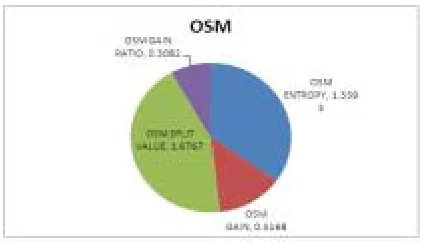
Figure - 2 Output values for given attributes
This Fig 2 shows the calculated value of entropy, gain, split value and gain ratio for the given attributes. The attribute OSM has the maximum gain value, so it is the root node of the decision tree.
These calculations will be continued until all the data classification has been done or else till all the given attributes get over.
5. CONCLUSION
The main concept of this research paper, is to improve the student’s performance in an efficient way by using Classification Technique in Data Mining. The concept of Decision Tree which integrates with the classification technique helps to achieve the goal by extracting the discovery of knowledge from the end semester mark. The inclusion of extracurricular activities makes to gain more knowledge along with the End semester Mark. This technique is one of the ways to improve performance of the students in education.
This section will help the teacher to predict those students who have the lesser performance; teacher can
develop them with special attention. This study will help these students to improve with confidence.
REFERENCES
[1]. Brijesh Kumar Baradwaj, Saurabh pal “Mining Educational Data to Analyze Students Performance”, IJACSA, Vol.2, No.6, 2011.
[2]. Heikki, Mannila, “Data mining: machine learning, statistics, and databases”, IEEE, 1996.
[3]. Toon calders SIGKDD Explorations “Introduction to the Special Section on Educational Data Mining” Volume 13, Issue 2.
[4]. U . K. Pandey, and S. Pal, “Data Mining: A prediction of performer or underperformer using classification”, (IJCSIT) International Journal of Computer Science and Information Technology, Vol. 2(2), pp.686-690, ISSN:0975-9646, 2011. [5]. Galit.et.al, “Examining online learning processes
based on log files analysis: a case study”. Research, Reflection and Innovations in Integrating ICT in Education 2007.
[6]. M. Bray, “The shadow education system: private tutoring and its implications for planners”, (2nd ed.), UNESCO, PARIS, France, 2007.
[7]. U. K. Pandey, and S. Pal, “A Data mining view on class room teaching language”, (IJCSI) International Journal of Computer Science Issue, Vol. 8, Issue 2, pp. 277-282, ISSN:1694-0814, 2011.
[8]. Z. N. Khan, “Scholastic achievement of higher secondary students in science stream”, Journal of Social Sciences, Vol. 1, No. 2, pp. 84-87, 2005.. [9]. J. Han and M. Kamber, “Data Mining: Concepts
and Techniques,” Morgan Kaufmann, 2000. [10]. Shaeela Ayesha, Tasleem Mustafa, Ahsan Raza
Sattar, M. Inayat Khan, “Data mining model for higher education system”, Europen Journal of Scientific Research, Vol.43, No.1, pp.24-29, 2010. [11]. B.K. Bharadwaj and S. Pal. “Data Mining: A
prediction for performance improvement using classification”, International Journal of Computer Science and Information Security (IJCSIS), Vol. 9, No. 4, pp. 136-140, 2011.
[12]. Q. A. AI-Radaideh, E. W. AI-Shawakfa, and M. I. AI-Najjar, “Mining student data using decision trees”, International Arab Conference on Information Technology(ACIT'2006), Yarmouk University, Jordan, 2006.