Canonical Correlation Analysis And Network Data Modeling: Statistical And Computational Properties

University of Pennsylvania

ScholarlyCommons

Publicly Accessible Penn Dissertations

2017

Canonical Correlation Analysis And Network Data

Modeling: Statistical And Computational

Properties

Zhuang Ma

University of Pennsylvania, [email protected]

Follow this and additional works at:

https://repository.upenn.edu/edissertations

Part of the

Statistics and Probability Commons

Recommended Citation

Ma, Zhuang, "Canonical Correlation Analysis And Network Data Modeling: Statistical And Computational Properties" (2017).

Canonical Correlation Analysis And Network Data Modeling: Statistical

And Computational Properties

Abstract

Classical decision theory evaluates an estimator mostly by its statistical properties, either the closeness to the underlying truth or the predictive ability for new observations. The goal is to find estimators to achieve statistical optimality. Modern "Big Data" applications, however, necessitate efficient processing of large-scale ("big-n-big-p'") datasets, which poses great challenge to classical decision-theoretic framework which seldom takes into account the scalability of estimation procedures. On the one hand, statistically optimal estimators could be computationally intensive and on the other hand, fast estimation procedures might suffer from a loss of statistical efficiency. So the challenge is to kill two birds with one stone. This thesis brings together

statistical and computational perspectives to study canonical correlation analysis (CCA) and network data modeling, where we investigate both the optimality and the scalability of the estimators. Interestingly, in both cases, we find iterative estimation procedures based on non-convex optimization can significantly reduce the computational cost and meanwhile achieve desirable statistical properties.

In the first part of the thesis, motivated by the recent success of using CCA to learn low-dimensional feature representations of high-dimensional objects, we propose novel metrics which quantify the estimation loss of CCA by the excess prediction loss defined through a prediction-after-dimension-reduction framework. These new metrics have rich statistical and geometric interpretations, which suggest viewing CCA estimation as estimating the subspaces spanned by the canonical variates.

We characterize, with minimal assumptions, the non-asymptotic minimax rates under the proposed error metrics, especially how the minimax rates depend on the key quantities including the dimensions, the condition number of the covariance matrices and the canonical correlations. Finally, by formulating sample CCA as a non-convex optimization problem, we propose an efficient (stochastic) first order algorithm which scales to large datasets.

In the second part of the thesis, we propose two universal fitting algorithms for networks (possibly with edge covariates) under latent space models: one based on finding the exact maximizer of a convex surrogate of the convex likelihood function and the other based on finding an approximate optimizer of the original non-convex objective. Both algorithms are motivated by a special class of inner-product models but are shown to work for a much wider range of latent space models which allow the latent vectors to determine the

connection probability of the edges in flexible ways. We derive the statistical rates of convergence of both algorithms and characterize the basin-of-attraction of the non-convex approach. The effectiveness and efficiency of the non-convex procedure is demonstrated by extensive simulations and real-data experiments.

Degree Type Dissertation

Degree Name

Doctor of Philosophy (PhD)

First Advisor Dean P. Foster

Second Advisor Zongming Ma

Keywords

Canonical Correlation Analysis, computational efficiency, dimension reduction, minimax rates, network data modeling, non-convex optimization

CANONICAL CORRELATION ANALYSIS AND NETWORK DATA MODELING:

STATISTICAL AND COMPUTATIONAL PROPERTIES

Zhuang Ma

A DISSERTATION

in

Statistics

For the Graduate Group in Managerial Science and Applied Economics

Presented to the Faculties of the University of Pennsylvania

in

Partial Fulfillment of the Requirements for the

Degree of Doctor of Philosophy

2017

Supervisor of Dissertation

Dean P. Foster

Marie and Joseph Melone Professor Professor Emeritus of Statistics

Co-Supervisor of Dissertation

Zongming Ma

Associate Professor of Statistics

Graduate Group Chairperson

Catherine Schrand, Celia Z. Moh Professor, Professor of Accounting

Dissertation Committee

Dean P. Foster, Marie and Joseph Melone Professor, Professor Emeritus of Statistics Zongming Ma, Associate Professor of Statistics

CANONICAL CORRELATION ANALYSIS AND NETWORK DATA MODELING:

STATISTICAL AND COMPUTATIONAL PROPERTIES

c

ACKNOWLEDGEMENTS

The last four years as a Ph.D. student have been a special and memorable journey with

mixed ups and downs, which I cannot possibly finish without tremendous and unconditional

love and support from my advisors, friends and families.

First and foremost, I would like to express my sincere gratitude to my advisors Dean Foster

and Zongming Ma for their guidance, encouragement and trust, which have made me an

independent researcher. I was given maximum freedom to explore research topics I am

passionate about. The discussions with them are always inspiring and stimulating. Thank

Dean for bringing me to areas beyond classical statistics and raising my interest in natural

language processing and deep learning. Thank Zongming for introducing me to network

data modeling which interlaces statistics, optimization and real data analysis.

I am also deeply grateful to Lawrence Brown and Robert Stine for sitting in my thesis

committee, being great collaborators and sharing their wisdom in both research and life.

In particular, I thank Bob for constantly encouraging and reminding me to pursue what I

am truly passionate about. I would also like to thank Michael Collins for hosting me at

Google Research and being a great mentor. Mike has showed me how theoretical intuitions

and domain knowledge could be transformed into state-of-art empirical results. I learned

enormously from his expertise in natural language processing and methods of scientific

research.

I am very fortunate to have collaborated with many senior colleagues in the department.

They generously shared their personal experience and offered me valuable suggestions which

have smoothed my research path. Special thanks go to Xiaodong Li, Yichao Lu and Asaf

Weinstein. Xiaodong is a role model and always pursues deeper understanding and sharper

Thanks go to all my friends at Penn, including but not limited to Sameer Deshpande, Wenjie

Dou, Zijian Guo, Colman Humphrey, Kwon Sang Lee, Shaokun Li, Xinyao Ji, Matt Olson,

Peichao Peng, Xin Lu Tan and Linjun Zhang. In particular, I thank Peichao for his help

all the way through.

Thanks also go to my high school and college friends, especially Kaifeng Chen, Huan He,

Yang Kang, Lin Li, Weifeng Sun, Jie Wang, Jun Wang, Jian Yin, Xun Zhang, Ke Zhao, and

Yunqing Zheng, for all the old days we spent together. It is always delightful and refreshing

when those memories come up every now and then.

Finally, I am indebted to my parents Donglei Ma and Yuanying Zhang for their continuing

love and support. They are the ultimate source of my strength and confidence.

Zhuang Ma

Philadelphia, PA

ABSTRACT

CANONICAL CORRELATION ANALYSIS AND NETWORK DATA MODELING:

STATISTICAL AND COMPUTATIONAL PROPERTIES

Zhuang Ma

Dean P. Foster

Zongming Ma

Classical decision theory evaluates an estimator mostly by its statistical properties, either

the closeness to the underlying truth or the predictive ability for new observations. The

goal is to find estimators to achieve statistical optimality. Modern “Big Data” applications,

however, necessitate efficient processing of large-scale (“big-n-big-p”) datasets, which poses

great challenge to classical decision-theoretic framework which seldom takes into account

the scalability of estimation procedures. On the one hand, statistically optimal estimators

could be computationally intensive and on the other hand, fast estimation procedures

might suffer from a loss of statistical efficiency. So the challenge is to kill two birds with

one stone. This thesis brings together statistical and computational perspectives to study

canonical correlation analysis (CCA) and network data modeling, where we investigate both

the optimality and the scalability of the estimators. Interestingly, in both cases, we find

iterative estimation procedures based on non-convex optimization can significantly reduce

the computational cost and meanwhile achieve desirable statistical properties.

In the first part of the thesis, motivated by the recent success of using CCA to learn

low-dimensional feature representations of high-low-dimensional objects, we propose novel metrics

which quantify the estimation loss of CCA by the excess prediction loss defined through

a prediction-after-dimension-reduction framework. These new metrics have rich statistical

the non-asymptotic minimax rates under the proposed error metrics, especially how the

minimax rates depend on the key quantities including the dimensions, the condition number

of the covariance matrices and the canonical correlations. Finally, by formulating sample

CCA as a non-convex optimization problem, we propose an efficient (stochastic) first order

algorithm which scales to large datasets.

In the second part of the thesis, we propose two universal fitting algorithms for networks

(possibly with edge covariates) under latent space models: one based on finding the exact

maximizer of a convex surrogate of the non-convex likelihood function and the other based

on finding an approximate optimizer of the original non-convex objective. Both algorithms

are motivated by a special class of inner-product models but are shown to work for a

much wider range of latent space models which allow the latent vectors to determine the

connection probability of the edges in flexible ways. We derive the statistical rates of

convergence of both algorithms and characterize the basin-of-attraction of the non-convex

approach. The effectiveness and efficiency of the non-convex procedure is demonstrated by

TABLE OF CONTENTS

ACKNOWLEDGEMENTS . . . v

ABSTRACT . . . vi

LIST OF TABLES . . . x

LIST OF ILLUSTRATIONS . . . xii

CHAPTER 1 : Introduction . . . 1

1.1 Canonical Correlation Analysis . . . 1

1.2 Network Data Modeling . . . 3

1.3 Thesis Outline . . . 4

CHAPTER 2 : Canonical Correlation Analysis: Subspace Perspective and Minimax Rates . . . 6

2.1 Introduction . . . 6

2.2 Subspace Perspective: Excess Prediction Loss and Subspace Angles . . . 12

2.3 Minimax Upper and Lower Bounds . . . 19

2.4 Proof of Theorem 1 . . . 26

2.5 Proof of Theorem 2 . . . 28

2.6 Proof of Theorem 3 . . . 42

2.7 Proof of Technical Lemmas . . . 52

CHAPTER 3 : Canonical Correlation Analysis: Iterative Algorithm . . . 71

3.1 Introduction . . . 71

3.2 Algorithm: Augmented Approximate Gradient Descent . . . 74

CHAPTER 4 : Network Data Modeling . . . 94

4.1 Introduction . . . 94

4.2 Latent Space Models . . . 99

4.3 Two Model Fitting Methods . . . 102

4.4 Simulation Studies . . . 116

4.5 Real Data Examples . . . 121

4.6 Discussion . . . 130

4.7 Proofs . . . 133

LIST OF TABLES

TABLE 1 : Brief Summary of Datasets . . . 82

TABLE 2 : Proportions of mis-clustered nodes by different methods on three

LIST OF ILLUSTRATIONS

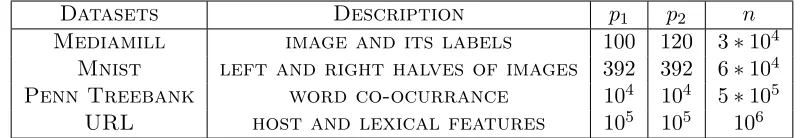
FIGURE 1 : Proportion of Correlations Captured (PCC) by AppGrad and

stochasticAppGrad on different datasets . . . 86

FIGURE 2 : Total Correlations Captured (TCC) by NW-CCA, DW-CCA,

PCA-CCA and stochasticAppGrad on URL dataset. The dashed

lines indicate TCC for those heuristics and the colored dots denote

corresponding computational cost. Red arrow means log(FLOP)

of PCA-CCA is more than 33. . . 88

FIGURE 3 : log-log boxplot for relative estimation errors with varying network

size and latent space dimension. . . 118

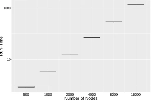
FIGURE 4 : log-log plot for average run time with varying network size. . . 118

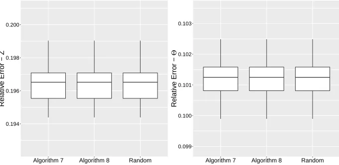
FIGURE 5 : Boxplot for relative estimation error with different initialization

methods. . . 119

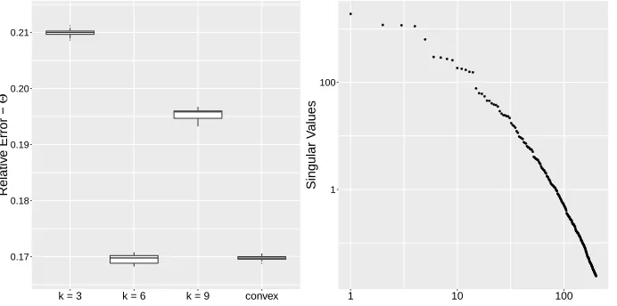
FIGURE 6 : log-log plot for the relative estimation errors of both convex and

non-convex approach under the distance kernelhd(zi, zj) =−kzi−

zjk. . . 120

FIGURE 7 : log-log plot for the relative estimation errors of both convex

and non-convex approach under the Gaussian kernel hg(zi, zj) =

4 exp(−kzi−zjk2/9) . . . 120

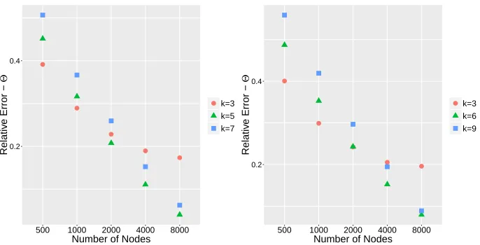
FIGURE 8 : log-log plot for the relative estimation error with varying network

size under distance kernelhd(zi, zj) =−kzi−zjk (left panel) and

under the Gaussian kernelhg(zi, zj) = 4 exp(−kzi−zjk2/9) (right

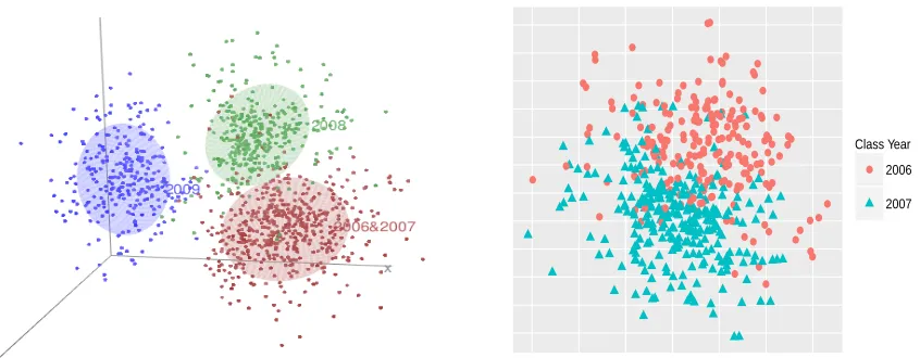
FIGURE 9 : The left panel is a visualization of the network with the first three

coordinates of the estimated latent vectors. The right panel is a

visualization of students in class year 2006 and 2007 by projecting

the four dimensional latent vectors to an estimated two dimensional

discriminant subspace. . . 125

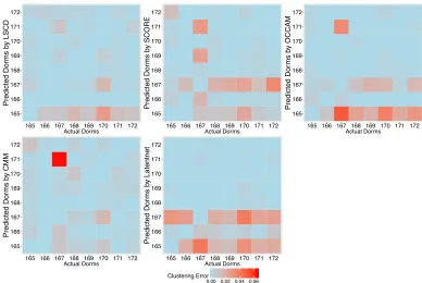
FIGURE 10 : Comparison of community-wise misclustering errors in Caltech

friendship network. Top row, left to right: LSCD, SCORE and

OCCAM; bottom row, left to right: CMM and Latentnet. . . 126

FIGURE 11 : Visualization of the lawyer network using the estimated two

dimensional latent vectors. The left panel shows results without

including any covariate while the right panel shows results that

used practice type information. . . 127

FIGURE 12 : Boxplots of misclassification errors using logistic regression with

different feature sets. We randomly split the dataset into training

and test sets with size ratio 3:1 for 500 times and computed

misclassification errors for each configuration. PC represents the

leading 100 principal components of the document-word matrix.

Z(k) represents the feature matrix where the ith row is the

concatenation of the estimated degree parameter α_bi and the

CHAPTER 1 : Introduction

The age of “Big Data” features cheap and easy availability of large quantities of

massive, high-dimensional, complex datasets, the analysis of which interlaces statistics,

machine learning and numerical optimization. The challenge/goal is to extract

low-dimensional structures from high-low-dimensional complex objects in a statistically optimal and

computationally efficient manner. This thesis brings together statistical and computational

perspectives in the study of canonical correlation analysis (CCA) and network data

modeling. We aim to answer questions such as:

What are the proper error metrics to quantify the estimation/prediction loss?

Under such metrics, what are the quantities that characterize the fundamental

statistical limits (e.g. the minimax rates)? To achieve the optimal error rates

on large datasets, what are the efficient algorithms?

1.1. Canonical Correlation Analysis

Canonical correlation analysis (CCA), first introduced by Hotelling (1936), is a fundamental

statistical tool to characterize the relationship between two groups of random variables and

finds a wide range of applications across many different fields. In recent years, CCA has

been successfully applied to learning low dimensional representations of high dimensional

objects like images (Rasiwasia et al., 2010), text (Dhillon et al., 2011) and speeches (Arora

and Livescu, 2013). Meanwhile, a parallel line of research builds up the theoretical fundation

for CCA to achieve sufficient dimension reduction (Kakade and Foster (2007); Foster et al.

(2008); Sridharan and Kakade (2008); Fukumizu et al. (2009); Chaudhuri et al. (2009) and

many others), especially under a popular multi-view setup.

Motivated by such empirical and theoretical success of CCA, we revisit CCA with a new

of CCA dates back to the study of the asymptotic distribution of the sample canonical

coefficients and sample canonical vectors like Hsu (1941), Izenman (1975), Anderson (1984,

1999) and many others. More recently, Chen et al. (2013) and Gao et al. (2014, 2015b)

established the non-asymptotic minimax rates of sparse CCA in a high dimensional setup.

Furthermore, there has been a surge of interest in developing scalable algorithms for

estimating CCA, to name a few, Avron et al. (2013) Lu and Foster (2014) (before the

proposed algorithm was published), Ge et al. (2016a), Wang et al. (2016) and Allen-Zhu

and Li (2016) (after the proposed algorithm was published).

Compared with previous work, our major contributions are as follows:

1. We propose novel metrics to quantify the estimation loss of CCA by the excess

prediction loss defined through a prediction-after-dimension-reduction framework.

These new metrics have rich statistical and geometric interpretations, which suggest

viewing CCA estimation as estimating the subspaces spanned by the canonical

variates.

2. We characterize, with minimal assumptions, the non-asymptotic minimax rates under

the proposed error metrics, especially how the minimax rates depend on key quantities

including the dimensions, the condition number of the covariance matrices and the

canonical correlations. To the best of our knowledge, this is the first finite sample

result that fully captures the effect of the canonical correlations on the minimax rates.

3. We propose an efficient (stochastic) first-order algorithm to compute the

leading-k dimensional sample canonical vectors. Compared with the well-known closed form

solution, the proposed iterative algorithm avoids multiplying/inverting/factoring large

1.2. Network Data Modeling

Network produces a prevalent form of data for quantitative and qualitative analysis in

many areas, including but not limited to sociology, engineering and neuroscience.

Real-world networks exhibit complex characteristics such as degree heterogeneity, transitivity,

homophily and community structure. These pose significant challenges to statistical

modeling. To date, researchers have proposed a collection of network models in various

fields. These models aim to catch different subsets of the foregoing characteristics, and

Goldenberg et al. (2010) provides a comprehensive overview. An important class of network

models are latent space models (Hoff et al., 2002). Suppose there are n nodes in the

observed network. The key idea underlying latent space modeling is that each node i

can be represented by a vectorzi in some low dimensional Euclidean space (or some other

metric space of choice) that is sometimes called the social space, and nodes that are “close”

in the social space are more likely to be connected. Hoff et al. (2002) considered two

types of latent space models: distance models and projection models. In both cases, the

latent vectors {zi}ni=1 were treated as fixed effects. Later, a series of papers (Hoff, 2003;

Handcock et al., 2007; Krivitsky et al., 2009) generalized the original proposal in Hoff et al.

(2002) for better modeling of other characteristics of social networks, such as clustering,

degree heterogeneity, etc. In these generalizations, the zi’s were treated as random effects

generated from certain multivariate Gaussian mixtures. Model fitting and inference in these

models has been carried out via Markov Chain Monte Carlo, and it is difficult to scale these

methodologies to handle large networks (Goldenberg et al., 2010). Moreover, one needs to

use different likelihood function based on choice of model and there is little understanding

of the quality of fitting when the model is mis-specified. Albeit these disadvantages, latent

space models are attractive due to their friendliness to interpretation and visualization.

We make progress on tackling the foregoing two issues simultaneously in this thesis, which

we summarize as the following main contributions:

are able to characterize degree heterogeneity, transitivity, homophily and community

structure. We design two fitting algorithms: one based on finding the exact maximizer

of a convex surrogate of the non-convex likelihood function and the other based on

directly finding an approximate optimizer of the non-convex objective. We derive high

probability error bounds for both algorithms and characterize the basin-of-attraction

of the non-convex optimization approach.

2. We show that these two fitting algorithms are “universal” in the sense that we are able

to establish their high probability error bounds for a wide range of latent space models

beyond the inner-product model class. For example, they work simultaneously for the

distance model and the Gaussian kernel model. Thus, the class of inner-product

models as well as the proposed fitting algorithms are indeed flexible and can be used

to approximate other latent space models of interest.

3. We demonstrate the effectiveness and efficiency of the model and algorithms on real

data examples for several different tasks, including visualization, community detection

and network-assisted learning. In particular, we obtain state-of-art performance for

the task of community detection on three benchmark datasets.

1.3. Thesis Outline

The reminder of the thesis is organized as follows. In Chapter 2, we propose new error

metrics which quantify the estimation loss of CCA by the excess prediction loss defined

through a prediction-after-dimension-reduction framework. This framework suggests

viewing CCA estimation as estimating the subspaces spanned by the canonical variates.

We also characterize, with minimal assumptions, the non-asymptotic minimax rates under

the proposed error metrics, especially how the minimax rates depend on the key quantities

including the dimensions, the condition number of the covariance matrices and the canonical

local linear convergence of the proposed algorithm.

In Chapter 4, we switch to the second part of the thesis: network data modeling. We propose

a special class of latent space models, called inner-product models, which could capture

typical characteristics of real-world networks. Then we propose two fitting algorithms based

on convex and non-convex optimization respectively. We further establish the statistical

rates of convergence of both algorithms and characterize the basin-of-attraction of the

non-convex approach. Finally, simulations and real-data experiments are provided to support

the proposed models and algorithms.

Chapter 2 and Chapter 3 are based on the paper Ma and Li (2016) and Ma et al. (2015)

respectively. Chapter 4 is based on the unpublished manuscript Ma and Ma (2017). My

research on shrinakge estimation (Ma et al. (2014a), Weinstein et al. (2015)) and reduced

CHAPTER 2 : Canonical Correlation Analysis: Subspace Perspective and Minimax

Rates

2.1. Introduction

Canonical correlation analysis (CCA), first introduced by Hotelling (1936), is a fundamental

statistical tool to characterize the relationship between two groups of random variables and

finds a wide range of applications across many different fields. For example, in genome-wide

association study (GWAS), CCA is used to discover the genetic associations between the

genotype data of single nucleotide polymorphisms (SNPs) and the phenotype data of gene

expression levels (Witten et al., 2009; Chen et al., 2012). In information retrieval, CCA is

used to embed both the search space (e.g. images) and the query space (e.g. text) into

a shared low dimensional latent space such that the similarity between the queries and

the candidates can be quantified (Rasiwasia et al., 2010; Gong et al., 2014). In natural

language processing, CCA is applied to the word co-occurrence matrix and generates vector

representations of the words which capture the semantics (Dhillon et al., 2011; Faruqui and

Dyer, 2014). Other applications, to name a few, include fMRI data analysis (Friman et al.,

2003), computer vision (Kim et al., 2007) and speech recognition (Arora and Livescu, 2013;

Wang et al., 2015).

The enormous empirical success motivates us to revisit the estimation problem of canonical

correlation analysis. From a decision-theoretic point of view, two questions are naturally

posed: What is the proper error metric to quantify the discrepancy between the population

CCA and its sample estimates? And under such a metric, what are the quantities that

characterize the fundamental statistical limits?

The justification of loss functions, in the context of CCA, has seldom appeared in the

literature. From the first principle that the proper metric to quantify the estimation loss

reduction. The first category, mostly in genomic research (Witten et al., 2009; Chen

et al., 2012), treats one group of variables as responses and the other group of variables

as covariates. The goal is to discover the specific subset of the covariates that are most

correlated with the responses. Such applications are characterized by low signal-to-noise

ratio and the interpretability of the results. The other category is investigated extensively

in statistical machine learning and engineering community where CCA is used to learn

low dimensional latent representations of complex objects such as images (Rasiwasia et al.,

2010), text (Dhillon et al., 2011) and speeches (Arora and Livescu, 2013). These scenarios

are usually accompanied by a relatively high signal-to-noise ratio and prediction accuracy,

using the learned low dimensional embeddings as a new set of predictors, is of primary

interest. In recent years, a series of publications has established fundamental theoretical

guarantees for CCA to achieve sufficient dimension reduction (Kakade and Foster (2007);

Foster et al. (2008); Sridharan and Kakade (2008); Fukumizu et al. (2009); Chaudhuri et al.

(2009) and many others), especially under a multi-view setup as will be discussed in detail

in Section 2.2.4.

In this thesis, we aim to address the problems raised above by treating CCA as a tool for

dimension reduction.

2.1.1. Linear Invariance of Canonical Variates

On the population level, CCA extracts the most correlated directions between two sets of

random variables: x∈Rp1 _{and y∈R}p2_{. To be specific, CCA recursively finds the pairs of}

vectors φi ∈Rp1,ψi ∈Rp2,1≤i≤p:= min{p1, p2} such that

(φi,ψi) = arg max

φ>_Σ

xφ=1,ψ>Σyψ=1

φ>Σxyψ

subject to φ>Σxφj = 0, ψ>Σyψj = 0, ∀ 1≤j≤i−1.

(2.1)

For 1≤i≤p, (φi,ψi) is theith pair of canonical coefficients (loading vectors), (φ>i x,ψ>i y)

Define Φ := [φ1,· · · ,φp], Ψ := [ψ1,· · · ,ψp] and Λ := diag(λ1,· · ·, λp). Then by definition,

Σx1/2Φ,Σy1/2Ψ have orthonormal columns and Λ = Φ>ΣxyΨ, which further implies that

Σx1/2Φ,Σ1y/2Ψ are respectively left and right singular vectors of Σx−1/2ΣxyΣ−y1/2. With these

notations, the first type of applications discussed above can be understood as identifying the

support of the top-kcanonical vectors: Φ1:kand Ψ1:k, where Φ1:k∈Rp1×kand Ψ1:k ∈Rp2×k

consist of the firstkcolumns of Φ and Ψ respectively. Dimension reduction, which motivates

this paper, is concerned with the leadingkcanonical variates: Φ>_1:kxand Ψ>_1:ky(kis assumed

to be pre-specified).

What distinguishes CCA from other dimension reduction methods like principal component

analysis or partial least squares is its linear invariance. As highlighted in Hotelling (1936)

when canonical correlation analysis was first developed:

The relations between two sets of variates with which we shall be concerned

are those that remain invariant under internal linear transformations of each set

separately.

Among all the population parameters, Hotelling (1936) noticed that the canonical

correlations λ1,· · · , λp and the functions of these quantities are the only linear invariants

of the system. On the contrary, the canonical coefficients Φ and Ψ will change accordingly

either with rotation of axes or scaling of the variables, which diminishes the rationale for

using an error metric built directly upon the loadings. If extending Hotelling’s notion

of invariants to include random vectors, the canonical variates are actually invariant

under linear transformations of each set separately. To illustrate, let T1, T2 be any pair

of nonsingular matrices and define the new random vectors a = T₁>x, b = T₂>y. As

will be shown in Section 2.3.1, T₁−1Φ1:k, T2−1Ψ1:k are the top-k canonical coefficients of

(a, b). Therefore, the top-k canonical variates of (a, b) will be (T₁−1Φ1:k)>a = Φ>1:kx and

(T₂−1Ψ1:k)>b = Ψ>1:ky, which are the same as those of (x, y). This fact substantiates our

What is the proper error metric to quantify the discrepancy between (Φ>_1:kx,Ψ>_1:ky) and the

sample counterparts (Φb>_1:kx,Ψb>_1:ky)? And under such a metric, what are the quantities that

characterize the fundamental statistical limits?

For the rest of the paper, we will focus on the relationship between Φb>_1:kx and Φ>_1:kx since

similar results can be obtained for the other pair by symmetry.

2.1.2. Subspace Estimation and Subspace Loss

In Section 2.2, we show that when CCA is used for dimension reduction, it is the difference

between the predictive power of Φ>_1:kx and Φb>_1:kx that matters, rather than the Euclidean

distance between Φ>_1:kxandΦb>_1:kx. Specifically, we characterize the discrepancy between the

predictive power by the excess prediction loss induced by replacing the population canonical

variates Φ>_1:kx with the sample estimatesΦb>_1:kx. When linear prediction is concerned, such

discrepancy is reduced to the difference between the linear span of the population and

sample canonical variates, denoted by span(x>Φ1:k) and span(x>Φb_1:k), which are subspaces

of span(x>) := {x>w, w ∈ _Rp1_{}. This suggests that CCA estimation can be viewed as}

subspace estimation, that is, estimating the subspace spanned by the leading-k canonical

variates: span(x>Φ1:k). From this perspective, the error metric L(·,·) we pursue could be

rewritten as

L(Φ>_1:kx,Φb>_1:kx) =L(span(x>Φ_1:k),span(x>Φb_1:k)). (2.2)

Interestingly, the error metrics derived through the excess prediction loss is closely related

to the principal angles (defined in Section 2.2.3) between span(x>Φb_1:k) and span(x>Φ_1:k).

Suppose θ = (θ1,· · ·, θk)> is the vector of such principal angles. As elaborated in

Theorem 1,

Worst case excess prediction loss'

P_Σ1_x/2Φb1:k −PΣ1x/2Φ1:k

2

=ksin(θ)k2_∞

Bayesian excess prediction loss'

P_Σ1_x/2Φb_1:k

−P_Σ1/2

x Φ1:k

2

F/2k=ksin(θ)k 2 2/k

where 'means ‘equal up to an absolute constant’, sin(θ) = (sin(θ1),· · ·,sin(θk)) and P(·)

denotes the projection matrix w.r.t. the column space of the matrix in the subscript.

2.1.3. Minimax Rates

In section 2.3, we characterize the non-asymptotic minimax estimation rates for CCA

under the error metrics proposed in (2.3), especially how the minimax rates depend on

the key quantities, including the dimensions, the condition number of the covariance

matrices and the canonical correlations. Informally, with operator norm error as an

example, in Theorem 2 and Theorem 3, we show that under certain a sample size condition

(n≥Cλk,λk+1(p1+p2)), the minimax rate is characterized by

inf

b

Φ1:k

sup

Σ∈FE

P_Σ1_x/2Φb1:k−PΣ1x/2Φ1:k

2

(1−λ

2

k)(1−λ2k+1)

(λk−λk+1)2

p1

n.

To the best of our knowledge, this is the first finite sample result that captures the factor (1−

λ2_k)(1−λ2_k+1). This term is not negligible becauseλk, λk+1are parameters depending on the

dimensions and should not be treated as constants. In practice, as the number of variables

increases, one should expect the canonical correlations to increase as well (e.g. considering

the case that the variables are gradually added to the two groups). The other important

feature is the independence of the dimensionp2. If only interested in the ‘estimation’ of the

canonical variates ofx, then even whenp2p1, as long as the sample size is large enough,

the minimax rate of ‘estimating’ Φ>_1:kx does not depend on p2. This phenomenon was also

revealed in Gao et al. (2014) and Cai and Zhang (2016) with the additional assumption that

all the residual canonical correlations are zero: λk+1=· · ·=λp1 = 0. Finally, the minimax

rates are independent of the condition number of the covariance matrices: κ(Σx), κ(Σy).

This is due to the linear invariance of the canonical variates as illustrated in Section 2.3.1.

We hope our theoretical findings could provide some guidance for the practical use of CCA

because in real applications, these factors matter both computationally and statistically

The upper bound of the minimax rates is achieved by sample CCA which is defined

in the same manner as (2.1) by replacing the population covariance matrices with the

corresponding sample estimates. The sample canonical variates are also linear invariant,

which is crucial in reducing the estimation error of sample CCA to the “standard form”, as

spelled out in Section 2.3.1, in which Σx and Σy are identity and Σxy = [Λ,0] (p1≤p2).

Theoretical understanding for the estimation of CCA dates back to the study of the

asymptotic distribution of sample CCA, in the low dimensional regime with fixed dimensions

and sample size going to infinity, for both sample canonical coefficients and sample canonical

correlations (Hotelling, 1936; Hsu, 1941; Izenman, 1975; Anderson, 1984, 1999) (and many

others). More recently, Chen et al. (2013) and Gao et al. (2014, 2015b) have studied the

non-asymptotic minimax rates of sparse CCA in a high dimensional setup. We defer the

detailed comparison between these results and ours to Section 2.3.2.

2.1.4. Notations

Throughout this chapter, we use lower-case and upper-case letters to represent vectors

and matrices respectively. For any matrix U ∈ _Rn×p _{and vector u ∈}

Rp, kUk,kUkF

denotes operator (spectral) norm and Frobenius norm respectively,kuk denotes the vector

l2 norm, U1:k denotes the submatrix consisting of the first k columns of U, and PU

stands for the projection matrix onto the column space of U. Moreover, we use σmax(U)

and σmin(U) to represent the largest and smallest singular value of U respectively, and

κ(U) =σmax(U)/σmin(U) to denote the condition number of the matrix. We use Ip for the

identity matrix of dimensionp and Ip,k for the submatrix composed of the firstk columns

of Ip. Further, O(m, n) (and simply O(n) when m = n) stands for the set of m×n

matrices with orthonormal columns andSp+denotes the set ofp×pstrictly positive definite

matrices. For a random vectorx∈_Rp_{, span(x}>_{) ={x}>_{w, w∈}

Rp}denotes the subspace of

all the linear combinations ofx. Other notations will be specified within the corresponding

2.2. Subspace Perspective: Excess Prediction Loss and Subspace Angles

In this section, we propose a prediction-after-dimension-reduction framework to quantify

the loss of any generic dimension reduction algorithm (including CCA). This framework

suggests two error metrics, one induced by the worst case excess prediction loss and the

other induced by the average excess prediction loss. For CCA, these two error metrics are

closely related to the principal angles between the subspaces spanned by the population

and sample canonical variates, respectively.

2.2.1. Linear Prediction Revisited

First, we review the basics of linear model theory under the random design setup. Suppose

given

x1, . . . , xp, z∈L2(Ω,F,P),

whereL2(Ω,F,P) is the set of random variables with mean zero and finite second moment,

and the goal is to predict the response z with the random vector x := (x1, . . . , xp)>. We

measure the prediction loss by

loss(z|x) := min

β∈_RpE[(z−x >

β)2].

We further assume that (x, z) has joint covariance matrix:

Cov 

  

  x

z 

 





=



 

Σx σxz

σ>_xz σ2_z 

 .

By classical linear model theory

β∗ := arg min

β∈RpE

[(z−x>β)2] = Σ−_x1σxz,

where rxz := Σ

−1/2

x σxz(σz2)−1/2 and krxzk2 is the population R2 which characterizes the

proportion of the variability in the response z explained by the predictor x. One notable

feature of such prediction loss is its linear invariance. Define the linear subspace spanned

by the coordinates ofx as

span(x>) :={x>w:w∈_Rp_{} ⊂L}2_(Ω,F,P).

If for another set of random variables{v1, . . . , vp} ∈L2(Ω,F,P) with span(v>) = span(x>)

and v:= (v1, . . . , vp)>, then by definition,loss(z|x) =loss(z|v). Therefore, we can rewrite

loss(z|x) =loss(z|span(x>)).

These two notations will be used interchangeably throughout the paper. The linear

invariance property can be revealed by noticing that krxzk2 = E[(Pspan(x)z)2]/E[z2] where

P₍·) is the projection operator defined in the Hilbert space L2(Ω,F,P) with covariance

operator as the inner product.

2.2.2. Competing with Oracles

Consider the scenario where the predictor x is in a high dimensional space and many

directions in span(x>) are redundant for predicting the response z. Practitioners usually

perform certain kind of dimension reduction on x before applying supervised learning

algorithms. SupposeU ∈Rp×k is a reduction matrix obtained by some generic dimension

reduction method. The subspace perspective of the prediction loss discussed in the previous

section suggestsloss(z|span(x>U))−loss(z|span(x>)), or simplyloss(z|span(x>U)) as the

measure of goodness for dimension reduction algorithms.

prediction loss can be quantified by:

loss(z|span(x>U1))−loss(z|span(x>U2)) =E[(Pspan(x>_U

2)z)

2_−(P

span(x>_U

1)z)

2_]

=σ2_z

r_xz>

P_Σ1/2

x U2 −PΣ1x/2U1

rxz

. (2.4)

The first equality is geometrically straightforward, measuring the proportion of the

variability in response z explained by the two subspaces: span(x>U1) and span(x>U2).

The algebraic expression in the second equality (proved in Theorem 1) is less obvious but

decouples the loss into an interaction between a supervised learning factor rxz and an

unsupervised learning factorP_Σ1/2

x U2−PΣ1x/2U1. To shed more light on this excess prediction risk, we parametrize the joint covariance matrix of (x, z) in terms of separate covariance

matrices Σx, σz2 and the vectorrxz, that is

Cov       x z      =   

Σx σxz

σ_xz> σ_z2   =   

Σ1x/2 0

0 σz

     

Ip rxz

r>_xz 1      

Σ1x/2 0

0 σz





. (2.5)

Considering the worst case discrepancy across all possible correlation structures, as proved

in Theorem 1,

sup

rxz:krxzk2=R2

n

loss(z|span(x>U1))−loss(z|span(x>U2))

o

=σ2_zR2

P_Σ1_x/2_U1 −P_Σ1_x/2_U2 ,

which suggests the right hand side of the equation as a sensible metric to quantify the

difference between the two reduction matrices. Actually, it is more informative to replace

the competitor U2 with an oracle reduction matrix, denoted by U?. As suggested by (2.4),

we say that a reduction matrixU? is an oracle reduction matrix ifP_Σ1/2

x U?rxz =rxz. Define

A := {r : P

Σ1x/2U?r = r,krk

2 _{= R}2_{} as the set of ‘correlation’ vectors such that U} ? is

prediction loss withinA, then according to Theorem 1,

sup

rxz∈A

loss(z|span(x>U))−loss(z|span(x>U?)) =σ2zR2

P_Σ1_x/2_U−P_Σ1_x/2_U?

2

. (2.6)

Interestingly, the operator norm is replaced by its square when the competitor is an oracle

reduction matrix. On the other hand, from a Bayesian perspective, considering the prior

that the vector rxz is sampled with respect to the uniform measure (Haar measure) onA,

denoted byπ, then the average excess prediction loss will satisfy (also refer to Theorem 1):

Erxz∼π

n

loss(z|span(x>U))−loss(z|span(x>U?))

o = σ

2 zR2

2k

P_Σ1_x/2_U −P_Σ1_x/2_U?

2

F. (2.7)

The analysis above connects the prediction loss for the generic response z with the

estimation loss for the oracle reduction matrix U? under the metrics derived in (2.6) and

(2.7). Therefore, when CCA is used for dimension reduction, it is natural to quantify the

discrepancy betweenΦb>_1:kx and Φ>_1:kx by the excess prediction loss:

P_Σ1_x/2Φb1:k−PΣ1x/2Φ1:k

2

,

P_Σ1_x/2Φb1:k−PΣ1x/2Φ1:k

2

F.

2.2.3. Measuring Subspace Distance by Principal Angles

In this section, we show that the loss defined in (2.6) and (2.7) are closely related to the

principal angles between the two subspaces spanned by the reduced predictors. For any

p dimensional random vector x with mean zero and bounded second moments, define the

Hilbert space

H= span(x>) ={X|X=x>w, w∈Rp}

with covariance operator as the inner product, that is, for any X1, X2 ∈ H, hX1, X2i

:= Cov(X1, X2) = E(X1X2). Suppose we have a pair of full column rank matrices

U1, U2 ∈ Rp×k and consider the canonical correlation analysis between the two subspaces

second, ..., and kth pair of canonical variates between span(x>U1) and span(x>U2).

Then span(W1, . . . , Wk) = span(x>U1), span(Wc1, . . . ,Wc_k) = span(x>U2) and hWi, Wji =

hWi,Wc_ji = hWc_i,cW_ji = 0, for any i 6= j and Var(W_i) = Var(cW_i) = 1, for i = 1, . . . , k.

Theith principal angle is defined asθi :=∠(Wi,Wc_i). Without loss of generality we assume

θ1≥ · · · ≥θk and define the distance between the two subspaces as:

L₂(span(x>U1),span(x>U2)) := k

X

i=1

sin2θi= k X i=1 1− D

Wi,Wc_i E

2

.

This is a valid metric because the principal angles are uniquely defined though the canonical

variates need not be. Sincex>Σ−x1/2is an orthonormal basis ofHunder the covariance inner

product, it is convenient to represent the elements in Hby this basis. Let

(W1, . . . , Wk) =x>Σ−x1/2B, and (Wc₁, . . . ,Wc_k) =x>Σ−_x1/2B,b

where B := [b1, . . . , bk], Bb := [bb₁, . . . ,bb_k]∈Rp×k are the coordinate representations under

x>Σ−x1/2. Notice that by definition, {W1, . . . , Wk}and{Wc₁, . . . ,Wc_k}are orthonormal bases

of span(x>U1) and span(x>U2), respectively. ThenB,Bbarep×kbasis matrices. Moreover,

we have b>_ibb_j =hW_i,Wc_ji= 0, for alli6=j.

Let’s now representL2(span(x>U1),span(x>U2)) in terms of B and Bb. In fact, since

1−

D

Wi,Wc_i E

2

= 1−

b

>

ibb_i 2 = 1 2 bib

>

i −bb_ibb>_i 2 F, we have

L2(span(x>U1),span(x>U2)) =

1 2 k X i=1 bib

>

i −bb_ibb>_i 2 F = 1 2 k X i=1

bib>i −bb_ibb>_i 2 F = 1

_BB>−_BB>

2

where the second equality is due to b>_i bj =bb>_i b_j =bb>_i bb_j = 0, for alli6=j.

Finally, notice that span(x>U1) = span(W1, . . . , Wk), x>U1 = (x>Σ−x1/2)(Σ1x/2U1), and

(W1, . . . , Wk) = x>Σ

−1/2

x B. Then B and Σ1x/2U1 have the same column space. Since

B ∈Rp×k is a basis matrix, we have BB>=P_Σ1/2

x U1, which is the orthogonal projector to the column space of Σ1x/2U1. Similarly, we haveBbBb>=P

Σ1x/2U2, which implies

L₂(span(x>U1),span(x>U2)) =

1 2

P_Σ1_x/2_U1 −P_Σ1_x/2_U2

2

F.

On the other hand, we can also define the distance through the largest principal angle:

L₁(span(x>U1),span(x>U2)) := sin2θ1= 1−

D

W1,Wc₁ E

2

.

Letθ= (θ1,· · ·, θk), then BB>BbBb>=Bdiag(cos(θ))Bb>, and by Lemma 2.18,

P_Σ1_x/2_U1 −P_Σ1_x/2_U2

2

=

BB

>₋ b BBb>

2

= 1−σ_min2 BB>BbBb>

= sin2(θ1) =L1(span(x>U1),span(x>U2))

We summarize the results into the following theorem of which the proof is deferred to

Section 2.4.

Theorem 1. Suppose(x, z)∼_Pfor some unknown distributionPwith covariance structure

specified in (2.5)and subspace angles defined above. For any pair reduction matricesU, U? ∈

Rp×k,

loss(z|span(x>U))−loss(z|span(x>U?)) =σz2

r>_xzP

Σ1x/2U?−PΣ1x/2U

rxz

sup

rxz: krxzk2=R2

loss(z|span(x>U))−loss(z|span(x>U?))

=σ_z2R2

P_Σ1_x/2_U−P_Σ1_x/2_U?

=σ

2

Let A={r :P

Σ1x/2U?r=r,krk

2_=R2_{}. By treatingU}

? as an oracle reduction matrix,

sup

rxz: rxz∈A

n

loss(z|span(x>U))−loss(z|span(x>U?))

o

=σ_z2R2

P_Σ1_x/2_U−P_Σ1_x/2_U?

2

=σ2_zR2ksin(θ)k2_∞.

By treating U? as a Bayes oracle, that is rxz ∼ π where π is the uniform measure (Haar

measure) onA, then

Erxz∼π

n

loss(z|span(x>U))−loss(z|span(x>U?))

o

= σ

2 zR2

2k

P_Σ1_x/2_U−P_Σ1_x/2_U?

2

F =

σ_z2R2

k ksin(θ)k

2 2

2.2.4. CCA for Multi-view Dimension Reduction

In the research and applications of multi-media analytics, data of the same object, is often

collected from multiple sources and exhibit heterogeneous properties. Features obtained

from different domains are referred to as different ‘views’. Usually each view summarizes a

specific aspect of the studied object and different views are complementary to one another.

For example, in web-page classification, the hyperlink structure and the words on the page

are two different views (Chaudhuri et al., 2009). In video surveillance, images of cameras

from different angles constitute different views (Loy et al., 2009). For more recent results,

see the survey paper of Xu et al. (2013) and references therein.

Although multiple views provide more potential discriminative information to distinguish

the patterns of different classes, the feature vector of each view usually lies in a high

dimensional space. It is critical, both statistically and computationally, to perform

dimension reduction before applying any supervised learning algorithm. It has been shown

(2008); Sridharan and Kakade (2008); Fukumizu et al. (2009); Chaudhuri et al. (2009) and

many others)

Suppose the input variablexcan be split into two viewsx(1), x(2) and the goal is to predict

the response z based on the two views. Let (Φ1:k,Ψ1:k) be the top-k population canonical

coefficients betweenx(1) and x(2). Foster et al. (2008) proved the following proposition.

Proposition 2.1. (Sufficient Dimension Reduction by CCA Foster et al. (2008)) Under

certain multi-view assumptions1,

loss(z|x(1)) =loss(z|span((x(1))>Φ1:k))

loss(z|x(2)) =loss(z|span((x(2))>Ψ1:k))

This proposition shows that the predictive power of the original high-dimensional predictors

x(1) _{and x}(2) _{is fully captured by the top k canonical variates. However, the proposition}

focuses on the population level and does not take into account the estimation error induced

by substituting the population canonical coefficients with the sample estimates. Such

sample-population discrepancy can be quantified by

loss(z|span((x(1))>Φb_1:k))−loss(z|span((x(1))>Φ_1:k)),

loss(z|span((x(2))>Ψb_1:k))−loss(z|span((x(2))>Ψ_1:k)),

or equivalently, the proposed loss functions according to Theorem 1.

2.3. Minimax Upper and Lower Bounds

In this section, we introduce our main results on non-asymptotic upper and lower bounds

for estimating CCA under the proposed loss functions. Specifically, the upper bound is

achieved by sample CCA.

2.3.1. Reduction for Sample CCA

In this section, we show that the linear invariance of both population and sample canonical

variates enables us to reduce the estimation error of sample CCA to the special case that

Σx=Ip1,Σy =Ip2 and Σxy = [Λ 0] (we assume p1 ≤p2 without loss of generality).

LetX = (x1,· · · , xn)> be the data matrix where x1,· · · , xn i.i.d

∼ N(0,Σx) and similarly we

defineY. It is well known that the top-k sample canonical coefficients can be defined as a

solution to the following optimization problem:

(Φb_1:k,Ψb_1:k)∈arg max

Wx,Wy

tr(W_x>Σb_xyW_y)

subject to W_x>Σb_xW_x=I_k, W_y>Σb_yW_y =I_k.

(2.8)

whereΣb_x,Σb_y,Σb_xy are sample variance and covariance matrices defined as

b Σxy =

1 nX

>_Y, b Σx =

1 nX

>_{X, and} b Σy =

1 nY

>_Y.

Coming back to the definition of population CCA in (2.1), Ψ is a p2 ×p1 matrix such

that Σ1y/2Ψ∈ O(p2, p1). In this section, we abuse notation and redefine Ψ as the p2×p2

matrix by arbitrarily padding the rest p2 −p1 columns such that Σy1/2Ψ ∈ O(p2). Let

ai = Φ>xi and bi = Ψ>yi. Then we will have ai i.i.d

∼ a= Φ>x with distributionN(0, Ip1)

and bi i.i.d

∼ b= Ψ>y with distributionN(0, Ip2). Moreover,

Σab:=Eaib>i = Φ

>

ΣxyΨ = (Σ1x/2Φ)

>

Σ−_x1/2ΣxyΣ−y1/2(Σ 1 2

yΨ) = [Λ 0].

where the last equality is due to the fact that Σ1x/2Φ,Σ1y/2Ψ are respectively left and right

singular vectors of Σ−x1/2ΣxyΣ

−1/2

y . This implies



  a

b 

 

i.i.d ∼ N



 0,



 

Ip1 Σab

Σ I



 



and their top-k population canonical coefficients (Φa_1:k,Ψb_1:k) = (Ip1,k, Ip2,k). Let A =

(a1,· · · , an)>=XΦ andB = (b1,· · ·, bn)>=YΨ. Then

b Σa=

1 nA

>_{A= Φ}> b ΣxΦ,

b Σb =

1 nB

>_{B = Ψ}> b ΣyΨ,

b Σab =

1 nA

>

B = Φ>Σb_xyΨ.

(2.9)

Since (Φb_1:k,Ψb_1:k) is a solution to the sample CCA (2.8), then

(Φ−1Φb_1:k,Ψ−1Ψb_1:k)∈arg max

Wx,Wy

tr(W_x>Φ>Σb_xyΨW_y)

subject to W_x>Φ>Σb_xΦW_x=I_k, W_y>Ψ>Σb_yΨW_y =I_k,

or, by (2.9), equivalently,

(Φ−1Φb_1:k,Ψ−1Ψb_1:k)∈arg max

Wx,Wy

tr(W_x>Σb_abW_y)

subject to W_x>Σb_aW_x =I_k, W_y>Σb_bW_y =I_k.

Therefore, (Φ−1Φb_1:k,Ψ−1Ψb_1:k) are the sample canonical coefficients for (a, b), which we

denote by (Φba_1:k,Ψb_1:b_k). Then a>Φba_1:k =x>Φb_1:k and a>Φa_1:k = x>Φ_1:k (linear invariance of

canonical variates). Hence,

P_Σ1_x/2_Φ1:k−P_Σ1_x/2Φb_1:k

2

=L₁(span(x>Φb_1:k),span(x>Φ_1:k))

=L1(span(a>Φba_1:k),span(a>Φa_1:k))

=

PΦa1:k −PΦba

1:k

2

.

By the same argument, with L1 replaced byL2,

P_Σ1_x/2_Φ1:k −P_Σ1_x/2Φb_1:k

2

F=

PΦa1:k−PΦba

1:k

2

F

[Λ 0] to analyze the estimation error of sample CCA.

Remark 2.2. As a byproduct, the reduction argument reveals that the estimation error

of sample CCA is independent of the condition numbers of the covariance matrices: κ(Σx)

and κ(Σy). This is not obvious because the separate estimation errors, kΣx−Σb_xk,kΣ_y−

b

Σyk,kΣxy−Σb_xyk, are in fact proportional to κ(Σ_x) and κ(Σ_y).

2.3.2. Upper and Lower Bounds

In this section, we assume x ∈ _Rp1_{, y ∈}

Rp2 are jointly normal with mean zero and joint

covariance matrix Σ specified by

Σ = 

 

Σx Σxy

Σ>_xy Σy



 

where Σx and Σy are nonsingular. Recall thatλ1,· · ·, λp1∧p2 are the canonical correlations

and (Φ,Ψ) are the canonical coefficient matrices (loadings) as defined in (2.1). For any

1≤k < p1∧p2, define thekth eigen-gap as ∆ =λk−λk+1.

Theorem 2. (Upper bound) There exists universal positive constantsC, C1, C2 independent

ofn, p1, p2 andΣsuch that if n≥C(p1+p2), the top-ksample canonical coefficients matrix

b

Φ1:k satisfies

E

P_Σ1_x/2Φb1:k −PΣ1x/2Φ1:k

2

≤C1

(1−λ2_k)(1−λ2_k+1) ∆2

p1

n +C2

p1+p2

n∆2

2

E

P_Σ1_x/2Φb1:k−PΣ1x/2Φ1:k

2

F/k

≤C1

(1−λ2_k)(1−λ2_k+1) ∆2

p1−k

n +C2

p1+p2

n∆2

2

The upper bounds forΨb_1:k can be obtained by switchingp₁ andp₂.

This theorem exhibits several notable features:

1. The multiplicative factor (1−λ2_k)(1−λ2_k+1)/∆2 appears in the principal term. The

between the two sets of random variables. When there is perfect correlation, that

is λk = 1, we can recover the CCA directions errorlessly because the observed data

along those directions are perfectly co-linear. The factor (1−λ2_k+1) comes as surprise

and appears in our lower bound as well. When λk is close to 1 and the eigen-gap ∆

is close to 0, for example, in the regime thatλk = 1−C∆, as ∆→0,

(1−λ2_k)(1−λ2_k+1)/∆2 constant

which indicates that consistency might still be achieved. In contrast, without the

factor (1−λ2

k+1), the principal term will explode since (1−λ2k)/∆2 1/∆. We

remark thatλk, λk+1 are parameters depending on the dimensions and should not be

treated as constants. As the number of variables increases, one should expect the

canonical correlations to increase as well (e.g. considering the case that the variables

are gradually added to the two groups).

To the best of our knowledge, this is the first finite sample result to capture the

factors: (1−λ2_k) and (1−λ2_k+1). This is achieved by a careful Taylor expansion of the

estimating equations for Φb_1:k and Ψb_1:k, inspired by the classical multivariate theory

of Anderson (1963, 1984, 1999) and Birnbaum et al. (2013), while the analysis of Gao

et al. (2014, 2015b) and Cai and Zhang (2016) does not yield this factor.

2. The dimension parameter p2 only appears in the high order term, which implies that

even whenp2 p1, as long as the sample size is large enough (see Corollary 2.4), the

‘estimation’ error of Φ>_1:kxwill not depend onp2. This phenomenon was first revealed

by Gao et al. (2014) through multi-stage estimation and sample splitting. The recent

work of Cai and Zhang (2016) directly proved such a result for sample CCA without

splitting the samples. The results of both Gao et al. (2014) and Cai and Zhang (2016)

are based on the artificial assumption that all the residual canonical correlations are

3. The upper bound does not depend on the condition number of the covariance matrices:

κ(Σx) and κ(Σy). It is directly implied by the reduction argument but not obvious

because the separate estimation errors, kΣx −Σb_xk,kΣ_y −Σb_yk,kΣ_xy −Σb_xyk, are in

fact proportional to these condition numbers. The success of the reduction argument

relies on the linear invariance of both population and sample canonical variates. For

loss functions directly based on the loadings (Chen et al., 2013; Gao et al., 2015b),

the upper bounds will be proportional toκ(Σx) andκ(Σy).

4. The only assumption made in Theorem 2 is that Σx,Σy are invertible. Anderson

(1999) assumes the canonical correlations are distinct because the argument requires

the asymptotic convergence of each individual canonical vector and coefficient.

Moreover, the result is asymptotic without finite sample guarantee. Gao et al. (2014)

and Cai and Zhang (2016) assumeλk+1 =· · ·=λp1 = 0, and Gao et al. (2014, 2015b)

assume the condition numberκ(Σx) andκ(Σy) are bounded.

To establish the minimax lower bound, we define the parameter space

F(p1, p2, k, λk, λk+1, κ1, κ2)

as the collection of joint covariance matrices Σ satisfying

Σx,Σy are nonsingular, κ(Σx) =κ1, κ(Σy) =κ2

0≤λp1∧p2 ≤ · · · ≤λk+1< λk≤ · · · ≤λ1 ≤1

We deliberately set κ(Σx) = κ1, κ(Σy) = κ2 to demonstrate that the lower bound is

independent of the condition number. For the rest of the paper, we will use the shorthand

F to represent this parameter space for simplicity.

and Σsuch that

inf

b

Φ1:k

sup

Σ∈FE

P_Σ1_x/2Φb1:k−PΣ1x/2Φ1:k

2

≥c2 (

(1−λ2_k)(1−λ2_k+1) ∆2

p1−k

n !

∧1∧p1−k

k )

inf

b

Φ1:k

sup

Σ∈FE

P_Σ1_x/2Φb1:k −PΣ1x/2Φ1:k

2 F/k

≥c2 (

(1−λ2_k)(1−λ2_k+1) ∆2

p1−k

n !

∧1∧p1−k

k )

where ∆ =λk−λk+1. The lower bounds for Ψb_1:k can be obtained by switching p₁ and p₂.

The proof of the lower bound is deferred to Section 2.6.

Remark 2.3. The upper and lower bounds together imply that the condition numbers of

Σx and Σy are neither cursing nor blessing when subspace estimation is concerned.

Gao et al. (2015b) obtained minimax lower bounds for sparse CCA in high dimensional

regime. Rephrasing their results without sparsity assumptions, they essentially proved

E

inf

Q∈O(p1)

E

x

>_Φ

1:k−x>Φb_1:kQ 2 F/k

≥c2

1−λ2_k κ1λ2_k

p1−k

n

∧1∧p1−k

k

,

with the parameter space λp1∧p2 = · · · = λk+1 = 0 < λk ≤ · · · ≤ λ1 ≤ 1. The inner

expectation is with respect to an independent samplex and the outer expectation is with

respect to the data from whichΦb_1:kis constructed. The inverse dependency on the condition

number in their results can be removed by noticing that

inf

Q∈O(p1)

E

x

>

Φ1:k−x>Φb_1:kQ 2 F ≥ 1 2

P_Σ1_x/2Φb1:k −PΣ1x/2Φ1:k

2

F.

(see Section 2.7.9 for the proof) and applying Theorem 3 with λk+1 = 0.

Corollary 2.4. When p1 ≥2k and

p1+p2

n∆2 ≤c

(1−λ2_k)(1−λ2_k+1) (1 +p2/p1)

for some universal positive constant c, the minimax rates can be characterized by

inf

b

Φ1:k

sup

Σ∈FE

P_Σ1_x/2Φb1:k−PΣ1x/2Φ1:k

2

(1−λ

2

k)(1−λ2k+1)

∆2

p1

n,

inf

b

Φ1:k

sup

Σ∈FE

P_Σ1_x/2Φb_1:k

−P_Σ1/2

x Φ1:k

2

F/k

(1−λ

2

k)(1−λ2k+1)

∆2

p1

n.

where ∆ =λk−λk+1.

Remark 2.5. For consistency, we only need the left hand side of (2.10) to converge to zero.

However in order for the high order term to be dominated by the principal term, the left

hand side of (2.10) is required to converge to zero faster than the right hand side.

2.4. Proof of Theorem 1

For anyU1, U2 ∈Rp×k, from classical linear model theory,

βi:= arg min

β E

z−β

>_(U>

i xi)

2

= (U_i>ΣxUi)−1Ui>σxz, i= 1,2,

and

loss(z|span(x>Ui)) =E[z2]−E[(βi>(Ui>xi))2]

=σ_z2−σ_xz>Ui(Ui>ΣxUi)−1Ui>ΣxUi(Ui>ΣxUi)−1Ui>σxz

=σ_z2

1−r_xz>(Σ_x1/2Ui)(Ui>ΣxUi)−1(Σ1x/2Ui)>rxz

.

Notice that (Σ1x/2Ui)(Ui>ΣxUi)−1/2 has orthonormal columns with column space

span(Σ1x/2Ui), then

loss(z|span(x>Ui)) =σ2z

1−r>_xzP_Σ1/2

x Uirxz

.

By the variational definition of the leading eigenvalue,

sup

rxz:krxzk2=R2

loss(z|span(x>U1))−loss(z|span(x>U2)) =σz2R2λmax

P_Σ1/2

x U2−PΣ1x/2U1

=σ_z2R2

P_Σ1_x/2_U2 −P_Σ1_x/2_U1 ,

where the second equality is by the characterization of the difference between two projection

matrices due to Wedin (1983). This proves the first claim of the theorem. For the second

part, sincerxz∈ A,

loss(z|span(x>U))−loss(z|span(x>U?))

=σ_z2r_xz> P

Σ1x/2U?−PΣ1x/2U

rxz

=σ_z2r_xz>P

Σ1x/2U?

P

Σ1x/2U?−PΣ1x/2U

P

Σ1x/2U2rxz

=σ_z2r_xz>P_Σ1/2

x U?

Ip−P_Σ1/2

x U

P_Σ1/2

x U?rxz

≤σ_z2R2

P_Σ1_x/2_U?

Ip−P_Σ1/2

x U

P

Σ1x/2U?

=σ_z2R2

P_Σ1_x/2_U?

Ip−P_Σ1/2

x U

2

=σ_z2R2

P_Σ1_x/2_U?−P_Σ1_x/2_U

2

.

Notice thatP

Σ1x/2U?

Ip−P_Σ1/2

x U

P

Σ1x/2U?is positive definite. Letu1 be the leading singular

vector of this matrix and definer∗_xz =Ru1. Then r∗xz ∈ Aand with such choice of r∗xz, the

inequality above will become equality and this implies that

sup

r∗ xz∈A

n

loss(z|span(x>U))−loss(z|span(x>U?))

o

=σ2_zR2

P_Σ1_x/2_U−P_Σ1_x/2_U?

2

.

For the last part of the theorem, let P

Σ1x/2U? =QQ

>_{. Then the setA can be rewritten as}

A={r :r=RQer, re∈S

The uniform measure (Haar measure)π onA can be defined through the uniform measure

(Haar measure) π_e on the sphere Sk−1. Because eπ is uniform on the sphere S

k−1_{, then}

Var(_eπ) =Ik/k (by symmetry) and

E

rxz∼π

h

loss(z|span(x>U))−loss(z|span(x>U?))

i

=σ2_zR2 Ere∼πe

h

e

r>Q>P

Σ1x/2U?−PΣ1x/2U

Q_eri

=σ2_zR2tr

Q>

P_Σ1/2

x U?−PΣ1x/2U

Q

/k

=σ2_zR2tr

P_Σ1/2

x U?−PΣ1x/2U

QQ>

/k

=σ2_zR2trIp−P_Σ1/2

x U

P

Σ1x/2U?

/k

Notice that P_Σ1/2

x U?=P

2 Σ1x/2U?

,

E

rxz∼π

h

loss(z|span(x>U))−loss(z|span(x>U?))

i

=σ2_zR2trP

Σ1x/2U?

Ip−P_Σ1/2

x U

P

Σ1x/2U?

/k

=σ2_zR2

P_Σ1_x/2_U?

Ip−P_Σ1/2

x U 2 F/k

=σ2_zR2

P_Σ1_x/2_U−P_Σ1_x/2_U?

2

F/2k,

where the last equality is due to Lemma 2.18.

2.5. Proof of Theorem 2

Throughout the proof, we assume p1 = p2 for the ease of presentation and the same

argument works for any p1 and p2 at the cost of heavier notations (when p1 6= p2, in

the definition (2.14), Λ2,Λb₂ will be rectangular instead of square matrices. As a result, the

subsequent places where Λ2 appears in the current proof should be understood as either Λ2

or Λ>₂ according to the dimensions in the specific context). We will still usep1, p2 (p1 ≤p2)