ALGORITHMS FOR BIVARIATE SINGULARITY ANALYSIS

(1)

Timothy DeVries

A Dissertation

in

Mathematics

Presented to the Faculties of the University of Pennsylvania in Partial Fulfillment of the Requirements for the Degree of Doctor of Philosophy

2011

Supervisor of Dissertation:

Robin Pemantle, Merriam Term Professor of Mathematics

Graduate Group Chairperson:

Jonathan Block, Professor of Mathematics

Dissertation Committee:

Herman Gluck, Professor of Mathematics

(2)

Acknowledgments

There are many people without whom this thesis would not exist, not least among whom are the professors I have worked with while a student at the University of Pennsylvania. I am eternally grateful to my advisor Robin Pemantle. Robin was a perfect advisor, quickly ascertaining both my strengths and my interests and guiding my research accordingly. I would also like to thank Mark Ward, in whose course I was first exposed to the joys of symbolic combinatorics. Together, Robin and Mark have opened a special place in my life for analytic combinatorics.

In the course of working on my thesis I have had the chance to work with and learn from many brilliant mathematicians. I thank Mark Wilson and Alex Raichev for producing the seed from which the first two chapters of this thesis grew. I thank Joris van der Hoeven for his work on rigorous numerics, and for our upcoming collaboration on implementing the algorithms described in this paper. I thank Philippe Flajolet and Robert Sedgewick for writingAnalytic Combinatorics, the book that reignited by interest in discrete math.

(3)

math department, things would have been a mess. Janet Burns, Monica Pallanti, Robin Toney and Paula Scarborough: I thank you.

Of course I would not be studying mathematics at all without the influence of many outstanding educators. Specifically, I would like to thank Carolyn Petite and Wade Tolleson, my high school computer science and calculus teachers, respectively. Their encouragement came at a critical time in my life, and gave me confidence in my abilities. I am also indebted to Louis Billera, whose course in combinatorics at Cornell steered my main mathematical interest.

I would like to give my sincerest thanks to my family. My father, Paul DeVries, and my mother, Emily DeVries, have supported me in every decision I have made. They provided me with every opportunity and trusted me to make the right choices. I thank my Dad for always being available to listen to and help with my (non-math) problems. I thank my brother Chris DeVries for sharing his knowledge of academia, and for understanding the trials I have faced. I thank my brother Matt DeVries for taking me backstage and forcing me to have fun every once in a while.

(4)

ABSTRACT

ALGORITHMS FOR BIVARIATE SINGULARITY ANALYSIS

Timothy DeVries Robin Pemantle, Advisor

An algorithm for bivariate singularity analysis is developed. For a wide class of bivariate, rational functions F =P/Q, this algorithm produces rigorous numerics for the asymptotic analysis of the Taylor coefficients ofF at the origin. The paper begins with a self-contained treatment of multivariate singularity analysis. The analysis itself relies heavily on the ge-ometry of the pole set _VQ of F with respect to a height function h. This analysis is then

(5)

List of Figures

2.1 The zero sets of Imf andf. . . 25

2.2 The branch cuts where parameterization by x fails. . . 26

2.3 The Riemann surface forp f(x). . . 26

2.4 A constructive view of the topology of_VQ. . . 28

2.5 The pentagonal path p. . . 32

3.1 The region _VQ local to σ0 with respect to height ˜h. . . 57

3.2 The region VQ local to σ0 with respect to height h. . . 57

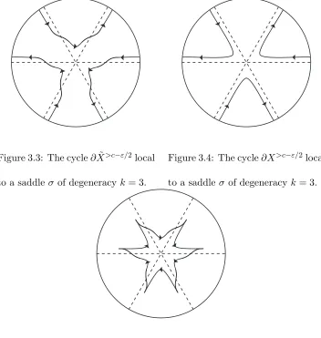
3.3 The cycle∂X˜>c−ε/2 _{local to a saddle}_σ _{of degeneracy}_k_{= 3. . . .} ₆₅

3.4 The cycle∂X>c−ε/2 local to a saddleσ of degeneracyk= 3. . . 65

3.5 The difference between the cycles∂X˜>c−ε/2 and ∂X>c−ε/2. . . 65

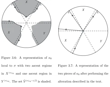
3.6 A representation of κ0 local to a saddleσ. . . 67

3.7 A representation of κ0 after preliminary alterations. . . 67

3.8 A representation of κafter final alterations. . . 68

(8)

Chapter 1

Singularity Analysis Background

1.1 Introduction

1

Let A denote a combinatorial class, i.e. a set of combinatorial objects. For example, A could be the set of all trees of a particular type, or the set of all walks on a two-dimensional grid having a particular structure, or any other manner of combinatorial object. We assume thatA admits a natural partition into a collection of finite subsetsAr indexed byd-tuples r= (r1, . . . , rd) of natural numbers. For example Ar could denote the set of trees with r1 nodes (indexed by 1-tuples), or the set of paths on anr1 by r2 grid (indexed by 2-tuples), etc. The main task in enumerative combinatorics is to count the objects of_Aby obtaining formulas for the sizes ar := |Ar| of these partitions. Often it is difficult to obtain exact formulas for thear directly, and so instead we shall seek asymptotic approximations for the

ar asr→ ∞.

Our analysis begins with the construction of the ordinary generating function of the 1_{Portions of Chapters 1 and 2 were first published in Contemporary Mathematics in volume 520, published}

(9)

class_A, which is the d-variable formal power series defined by

F(x) = X r∈Nd

arxr

(wherexr is shorthand for xr1

1 · · · · ·xrdd ). The combinatorial structure ofAoften reveals F

to be an analytic function in a neighborhood of the origin 0_∈Cd, leading to a closed-form representation forF. It is then hoped that analytic properties ofF may be used to extract information about its coefficients, freeing the problem from its discrete roots and opening it up to the techniques of analysis. This method is known as singularity analysis, due to the strong relationship between the asymptotic growth of the coefficients ar and the singular set of the generating functionF.

Singularity analysis in the univariate, d = 1 case has been studied thoroughly (see [FS09]) and is well understood, e.g. formulas exist for computing asymptotics for univari-ate generating functions that are rational, algebraic-logarithmic, or even of several more complicated or implicitly defined classes. The multivariate, d_≥2 case is far less well un-derstood. Recently, however, a line of research begun by Robin Pemantle and Mark Wilson (see [PW02] and [PW08]) has proved to be a fruitful generalization of singularity analysis to higher dimensions.

The singularity analysis of Pemantle and Wilson has the following basic structure: be-gin with Cauchy’s Integral Formula, manipulate the integral/integrand, and end with sad-dle point integration. To be more explicit, we assume that the generating function of a particular combinatorial class takes the form F = η/Q, with η : Cd _→ C entire and

Q ∈ Q[x1, . . . , xd]. Cauchy’s Integral Formula then expresses the coefficients of F as an

(10)

cycle _{C ⊆ V}Q.We define a height functionh on the varietyVQ related to the rate of decay

of this new integrand. We then push this cycle down alongVQ, minimizing the maximum

ofh along_C at critical points of the functionh.Under the right conditions, the coefficients can finally be approximated as saddle point integrals along _C in small neighborhoods of a finite set of these critical points, known as the contributing points. We shall study these techniques in more detail in the remainder of Chapter 1.

It is shown in [PW02] and [PW08] how these techniques produce automatic asymp-totic formulas for many bivariate rational generating functions. Specifically when all the contributing points areminimal — that is, on the generating function’s boundary of conver-gence — then an explicit algorithm exists for determining which critical points contribute and computing the saddle point integral near these points (in the bivariate case). And when the generating function iscombinatorial, i.e. when all its coefficients are non-negative, then the contributing points will all be minimal (under the standing assumption of [PW08], Assumption 3.6).

(11)

combinatorial; only along a diagonal do the coefficients in this new generating function actually count something, and off the diagonal the coefficients are free to be (and often are) negative.

In the non-combinatorial case, [PW02] does not provide us with the locations of the contributing points. Worse than that, however, is that even once the contributing points have been found, there is no formula automatically producing the correct saddle point computation in a neighborhood of these points. This is because the structure of _C local to the contributing points is not automatically known. (On the contrary, for minimal contributing points, an explicit construction for_C near these points is known; see [PW02]). This is particularly bad when the contributing point is a degenerate saddle point for the height function. Since the height on C is locally maximized at the contributing point, it must locally approach and depart along ascent and descent paths. A greater degree of degeneracy means more ascent/descent paths, hence more possibilities for the local path followed by C. And indeed in the case of bicolored supertrees the contributing point is a degenerate saddle point of the height function.

Understanding the saddle point integration near these degenerate saddles is particularly important because degenerate saddles arise frequently in combinatorial applications (despite the fact that they are nongeneric). A careful analysis of [PW02] reveals that, in the absence of such degenerate saddles, one obtains leading term asymptotics only of the form cAnnp/2

(12)

(see [FS09, Section VII.7]), and so a multivariate analysis of the corresponding bivariate rational function should turn up a degenerate saddle wheneverq >2.

In Chapter 3 we explore the topology of _VQ (for bivariate Q) and the homology class

of the cycle _C on _VQ. Under certain assumptions on Q and the height function h, we will

ultimately produce a topological characterization of the set of contributing points and of the structure of the cycle _C local to these points. This characterization is particularly nice in that it is effectively computable, though this is not obvious. Finally in Chapter 4 we use the topological characterization of Chapter 3 to present a fully implemented algorithm for locating the contributing points and describing the structure of_C local to these points. Note that portions of Chapters 3 and 4 will appear in a forthcoming work, [DPvdH11].

Chapter 2 is a case study in the techniques developed in the subsequent chapters. It shall serve as a motivating example for understanding how to apply singularity analysis to a possibly non-combinatorial rational generating functionF =P/Q. Though the results of Chapter 2 are subsumed in the later work, the intuition behind the more general results will be better understood after seeing an example. Note that the techniques applied to describe VQ in Chapter 2 are somewhat ad-hoc, and not appropriate for an automatic computation.

(13)

1.2 Coefficient representation

For the duration of this paper, let F :Cd_→Cbe a function analytic in a neighborhood of the origin, having representation

F(x) = X r∈Nd

arxr,

wherexris shorthand notation forxr1 1 . . . x

rd

d .The goal is to obtain an asymptotic expansion

for the coefficientsar given F,and the main tool for this is Cauchy’s Integral Formula.

Theorem 1.2.1 (Cauchy’s Integral Formula). Let F be as above, analytic in a polydisc

D0={x:|xj|< εj∀j},for some positive, real εj.Assume further that F is continuous on

the distinguished boundaryT0 ofD0, a product of loops around the origin in each coordinate, each one positively oriented with respect to the complex orientation of its respective plane. Then

ar =

Z

T0

ωF,

where

ωF =

1 (2πi)d ·

F(x)

x1·. . .·xd

x−rdx.

Cauchy’s Integral Formula can be found in most textbooks presenting complex analysis in a multivariable setting, and follows easily as an iterated form of the single variable formula. See, for example, [Sha92, p. 19].

We wish to use the structure of Cauchy’s formula to obtain an asymptotic formula for

(14)

Specifically, define the (d₋1)-simplex ∆d−1 _by

∆d−1 =

 



(ˆr1, . . . ,ˆrd) : ˆrj ≥0∀j, d

X

j=1 ˆ

rj =d

 



,

where we choose the convention that the ˆrj sum todfor later notational convenience. Then

anyrin the positived-hyperoctant can be written uniquely asr=_|r_|ˆr,where_|r_{| ∈}R+ and ˆ

r_∈∆d−1.We examineras|r_{| → ∞} and ˆr_→ˆr0 for some fixed direction ˆr0 ∈∆d−1. Now we turn to the structure of the integrand ωF, specifically x−r (the portion that

changes as we varyr). With an eye on the end goal of reducing our computation to a saddle integral, we use the following representation (away from the coordinate axes):

x−r= exp



−

d

X

j=1

rjlogxj



= exp (|r|H_ˆr(x)),

where we define the multi-valued function

Hˆr(x) :=−

d

X

j=1 ˆ

rjlogxj. (1.2.1)

When no confusion exists, we will simply refer to the function Hˆr as H. Now the over-all magnitude of the integrand will be an important factor in computing an asymptotic expansion forar,and so we next examine the magnitude of exp (|r|Hˆr(x)).We have

|exp (_|r_|Hˆr(x))|= exp (|r|ReHˆr(x)) = exp (|r|hˆr(x)),

where we define the single-valued function

hˆr(x) := ReHˆr =−

d

X

j=1 ˆ

rjlog|xj|. (1.2.2)

(15)

As _|r_{| → ∞}, the above equations show that the magnitude of the integrand grows at an exponentially slower rate along points further away from the origin (where the height functionhis smaller). This motivates pushing the domain of integration out towards infinity, reducing the growth rate of the integrand on the domain over which it is integrated. Of course ifF has poles they will present an obstruction, but we can still try push the domain of integration around these poles. In the end we obtain an integral over two domains: one near the pole set ofF (obtained by pushing the original domain around the poles), and one past the pole set of F (far away from the origin). This idea is formalized in the theorem below.

Theorem 1.2.2. Let F =P/Q, with P, Q:Cd_→ Centire, where the vanishing set _VQ of Q is smooth. Let T0 be a torus as in Cauchy’s Integral Formula. Let T1 ⊆Cd be a torus homotopic to T0 under a homotopy

K :T_×[0,1]_→Cd, withT0 =T× {0}, T1 =T× {1},

passing through _VQ transversely. Identifying K with its image in Cd, assume further that K does not intersect the coordinate axes, and that ∂K_{∩ V}Q=∅. Define

C =K_{∩ V}Q.

Then for any tubular neighborhood ν of of C in K, we have

ar=

Z

T0

ωF =

Z

∂ν ωF +

Z

T1

ωF,

given the proper orientation of ∂ν.

Note: when we say _VQ is smooth we mean that VQ has the structure of a smooth

(16)

mean that the image ofK intersects with_VQ transversely as (real) submanifolds ofCd (see

[Bre93, p. 84]).

Proof. Counting (real) dimensions, dim_VQ = 2d−2 and dimK = d+ 1. Hence their

transverse intersectionC is ad−1 real-dimensional subspace of K.

Now take any tubular neighborhoodν ofC inK.Asν is a full-dimensional submanifold of the orientable manifold K, ν is orientable and hence its boundary ∂ν is orientable too. Given the proper orientation of ∂ν, we have that

∂(K\ν) =T1−T0+∂ν.

Note that ωF is holomorphic on K\ν. By Stokes’ Theorem ([Bre93, p. 267]) and the

fact that ωF is an exact form we get

Z

T1−T0+∂ν

ωF =

Z

K\ν

dωF =

Z

K\ν

0 = 0,

leading to the equality of the theorem.

When T1 is far enough away from the origin,R_T₁ωF is negligible (possibly even 0), and so the asymptotic analysis of the coefficients ar reduces to an integral near the pole set of

F.In the next section, we reduce this further to an integral on the pole set of F.

1.3 The residue theorem

(17)

1.3.6 below, an analogue of the Cauchy Residue Theorem in one variable. Its application to coefficient analysis is found in Corollary 1.3.7.

We restrict our attention to a limited part of Leray’s theory, focusing on meromorphic

d-forms inCd.

Definition 1.3.1. Let η be a meromorphicd-form, represented as

η= P

Qdx on a domain U ⊆C d

where P and Q are holomorphic on U. Denote by _VQ the zero set of Q on U, and assume

thatηhas a simple pole everywhere on VQ.Denote byι:VQ→U the inclusion map. Then

we define the residue of η on _VQ by

Res(η) =ι∗θ,

whereι∗ denotes pullback byι(see [Bre93, p. 263]), and where θis any solution to

dQ_∧θ=P dx.

Before delving into the existence and uniqueness of the residue, we do a few example computations.

Example 1.3.2. For η=P/Q dx as above, wherever Qi = _∂xi∂Q does not vanish we have the

representation

Res(η) = (₋1)i−1P

Qi

dx1∧ · · · ∧dxi−1∧dxi+1∧ · · · ∧dxd.

As a special case, note that forQ=x1 we obtain

(18)

In the case whered= 1,this reduces to Res(P(x)/x) =P(0),which is precisely the ordinary residue of P(x)/x atx = 0. This motivates the above definition as a genuine extension of the single variable residue.

Example1.3.3. As the most pertinent case of the Example 1.3.2, we examine Res(ωF) where F =P/Qis meromorphic. Away from the coordinate axes,ωF can be written as

ωF =

1 (2πi)d ·

P(x)

x1...xdexp(|r|H(x))

Q(x) dx,

where the numerator and denominator are holomorphic functions. So whereverQdand the xj do not vanish (for all j), we have

Res(ωF) = (−1)

d−1 (2πi)d ·

P(x)

x1. . . xdQd(x)

e|r|H(x)dx1∧ · · · ∧dxd−1.

We now show existence and uniqueness of the residue form along the simple pole set VQ.

Proposition 1.3.4. Let η be as in Definition 1.3.1. Then for any pointp∈ VQ,there is a

neighborhood V _⊆U of p and a holomorphic (d₋1)-formθ on V solving the equation

dQ∧θ=P dx. (1.3.1)

Furthermore, the restriction ι∗θ induced by the inclusion ι:VQ∩V →V is unique.

Proof. First, we prove the existence of a solution θto (1.3.1) in a neighborhood ofp.AsQ

has a simple zero at p, the implicit function theorem implies that for some neighborhood

V of p there is a biholomorphic function ψ:Cd _→V such that Q(ψ(x)) =x1.Define the form θ0 by

(19)

where J is the Jacobian of the function ψ.The claim is thatθ= (ψ−1₎∗_θ₀ _{is a solution to} (1.3.1).

Indeed, by definition ofθ0we have thatdx1∧θ0= (P◦ψ)|J|dx.Pulling back both sides of this equation byψ−1 yields

d(ψ−1(x)1)∧(ψ−1)∗θ0=P·(ψ−1)∗(|J|dx),

which simplifies to dQ_∧θ=P dx,as desired.

To prove uniqueness, assume that we have two (d₋1)-formsθand ˜θsuch thatdQ_∧θ=

P dxand dQ∧θ˜=P dx.Then dQ∧(θ−θ˜) = 0,which implies

ψ∗(dQ∧(θ−θ˜)) =dx1∧ψ∗(θ−θ˜) = 0.

But this means thatψ∗(θ−θ˜) is a multiple ofdx1.Pulling back by (ψ−1)∗,this implies that

θ₋θ˜is a multiple ofdQ.Finally, pulling back byι∗_,_{this implies that}_ι∗₍_θ₋_θ˜_{) is a multiple} of d(Q_◦ι) = 0.Thus ι∗(θ₋θ˜) vanishes, and so ι∗θ=ι∗θ.˜

Remark 1.3.5. Let η be as in the definition of the residue form, and let ψ : V _→ U be a biholomorphic function. Then

1. The residue form is natural, i.e. Res(η) does not depend on the particular P and Q

chosen to representη as (P/Q)dx.

2. The residue form is functorial, i.e. Res(ψ∗η) = ψ∗Res(η) (where on the right side of the equation,ψ is restricted to the domain ψ−1₍_V

Q) =VQ◦ψ).

(20)

d-chain in U, locally the product of a (d₋1)-chain C on _V with a circle γ in the normal slice toV,oriented positively with respect to the complex structure of the normal slice. Then

Z

N

η = 2πi

Z

C

Res(η).

Proof. We proceed by examining the structure of the integral locally. So fix an arbitrary p ∈C. In a neighborhood V ⊆Cd of p,the surrounding space looks like a direct product of _{V ∩}V (isomorphic to Cd−1 for V small) and the normal space to _{V ∩}V (isomorphic to

C). Hence there is a biholomorphic function

ϕ:V →C_×Cd−1

x7→(ϕ1(x), ϕ2(x))

where the map ϕ−₂1 is a parametrization of _{V ∩}V, and

ϕ(V ∩V) ={0} ×ϕ2(V ∩V),

ϕ(N _∩V) =γ_×ϕ2(C∩V),

where γ _⊆C is a loop around the origin, positively oriented. Furthermore, if V is chosen small enough, we can guarantee that the meromorphic form (ϕ−1)∗η has a global represen-tation as P/Q dx.Note that, by the structure of η and definition of ϕ, Q must vanish on the set

ϕ(_{V ∩}V) =_{x_∈Cd:x1 = 0}, where it has only simple zeros.

I claim that if we can prove the equality stated in the residue theorem restricted to

(21)

compactness ofC: we can split up a tubular neighborhood ofC (containingN) into finitely many such neighborhoods on which the theorem holds, then prove the theorem by breaking the integral into a sum over these pieces.

So without loss of generality, we may assume that this local structure holds globally on

C and that the domain of the map ϕis all of Cd.By changing variables, we get

Z

N η =

Z

γ×ϕ2(C)

P Qdx=

Z

p∈ϕ2(C)

Z

γ×{p}

P Qdx1

!

dx2∧ · · · ∧dxd. (1.3.2)

the upshot being the ability to split the above into an iterated integral, by the product structure of γ×ϕ2(C).

The next step is to compute the inner integral from (1.3.2) by the ordinary residue theorem, but doing so will require a change of variables. To that end, define the function

ψ:Cd_→Cd by

ψ(x) = (Q(x), x2, x3, . . . , xd),

and fix some p _∈Cd−1.The claim is that ψ is biholomorphic in a neighborhood W _⊆Cd

of (0,p). By the inverse function theorem, this is true if and only if _|J(p)_| = Q1(p) 6= 0, whereJ is the Jacobian of ψ.AsQ has a simple zero atp,it can’t be true that Qi(p) = 0 for alli. ButQi(p) = 0 for alli6= 1,because Qis constant (equal to 0) on the entire plane x1 = 0.Thus Q1(p)6= 0,as desired. Note thatψ−1 must have the form

ψ−1(x) = (f(x), x2, x3, . . . , xd)

for some functionf, and thatQ_◦ψ−1=x1.

We’d like to perform a change of variables and compute the inner integral from (1.3.2) over the domainψ(γ_{× {}p_}).The only problem with this is that there is no guarantee that

(22)

closer to the origin, and by (potentially) restricting our attention to a small portion of C.

Note that shrinkingN has no effect on the original integral (the new N will differ from the oldN by a boundary, and we are integrating a closed form), and that, as we have already stated, we need only prove the residue theorem locally. Thus we may assume without loss of generality that γ×ϕ2(C) is contained entirely within the domain ofψ.

After the suggested change of variables, we obtain

Z

N η=

Z

p_∈ϕ2(C)

Z

ψ(γ×{p_})

P_◦ψ−1

x1

∂f ∂x1

dx1

!

dx2∧. . .∧dxn.

By the form of ψ, ψ(γ_{× {}p_}) is simply a loop around the origin in the plane _{x _∈ Cd : (x2, . . . , xd) =p}.So by the ordinary residue theorem we can compute

Z

ψ(γ×{p})

P _◦ψ−1 x1

∂f ∂x1

dx1 = 2πi·P(ψ−1(0,p))

∂f ∂x1

(0,p).

Substituting back into (1.3.2) yields

Z

N

η= 2πi

Z

p∈ϕ2(C)

P(ψ−1(0,p))∂f

∂x1

(0,p)dx2∧. . .∧dxn

= 2πi

Z

{0}×ϕ2(C)

Res P◦ψ −1_· ∂f

∂x1

x1

dx

!

,

where the second equality comes from the residue computation of Example 1.3.2. But note that

(ψ−1)∗

P Qdx

= P◦ψ− 1 x1   d X j=1 ∂f ∂xj dxj 

∧dx₂∧ · · · ∧dx_d

= P◦ψ− 1

x1

∂f ∂x1

dx,

and so the integral equation becomes

Z

N

η= 2πi

Z

{0}×ϕ2(C) Res

(ψ−1)∗

P Qdx

= 2πi

Z

{0}×ϕ2(C)

Res (ψ−1)∗(ϕ−1)∗η

(23)

Finally, by the functoriality of the residue form, we obtain

Z

N

η= 2πi

Z

{0}×ϕ2(C)

(ψ−1)∗(ϕ−1)∗Res(η) = 2πi

Z

C

Res(η).

The residue theorem applies directly to the coefficient analysis of the previous section by the following corollary.

Corollary 1.3.7. Under the assumptions and notation of Theorem 1.2.2

ar = 2πi

Z

C

Res(ωF) +

Z

T1

ωF,

given the proper orientation of C.

Proof. By the residue theorem,R

∂νωF = 2πi

R

CRes(ωF).The result follows by substituting

this equality into the conclusion of Theorem 1.2.2.

And thus the asymptotic coefficient analysis reduces to the integration of a d₋1 form along a cycle on the pole set of the coefficient generating function. The final step is to compute this integral by means of the saddle point method.

1.4 Critical points of the height function

The goal is to obtain an asymptotic expansion for 2πiR

CRes(ωF),whereF =P/Qfor some

entire functionsP and Q, F is analytic in a neighborhood of the origin, and_VQ is smooth.

By Example 1.3.3 we can expect Res(ωF) to take the form

Res(ωF) =

(₋1)d−1 (2πi)d ·

P(x)

x1. . . xdQd(x)

(24)

(where Qddoes not vanish), and as before we see that the exponential growth of this form

is governed by the height functionh.This motivates a deformation of the cycleC alongVQ,

pushingCdown to a homologous cycle ˜Con which the maximum modulus ofhis minimized. This procedure is obstructed when the cycle gets trapped on a saddle point of h on _VQ,

and the idea is to arrange ˜C so that the local maxima ofh along ˜C areall achieved at such saddle points. Away from the highest saddle points (the contributing points) the integral will contribute asymptotically negligible quantities, and near the contributing points the integral will be amenable to the saddle point method.

Thus the first task is to identify the location of the critical points of hˆr|VQ.We denote

this set of points by Σˆr, or simply by Σ when the direction ˆris understood. Then the points of Σˆr can be realized as the zero set ofdequations, as exhibited below.

Theorem 1.4.1 (Location of Critical Points). Assume ˆrd 6= 0. Then the set Σˆr consists precisely of the pointsp_∈Cd satisfying the followingd equations:

Q(p) = 0,

ˆ

rdpjQj(p)−rjˆpdQd(p) = 0 ∀j6=d.

In the case d= 2, these critical points are actually saddle points of hˆr|VQ.

For the purposes of computation it should be noted that when Q is a polynomial, the above set of critical points is generically finite and can be found algorithmically by the method of Gr¨obner bases (see [CLO05, Section 1.3]).

Proof. The equationQ(p) = 0 is clear: any critical point ofh_|_V_Q will have to be on_VQ.So

(25)

Fix a point p_{∈ V}Q (not on the coordinate axes). By the Cauchy-Riemann equations, p

is a critical point of Re H|VQ

if and only if it is a critical point of Im H|VQ

.Thus p is a critical point of h_|_V_Q exactly when

∇(H|VQ)(p) = 0.

But ∇(H|VQ)(p) is simply the projection of ∇H(p) onto the tangent space TpVQ. Hence

the previous equation is true if and only if

∇H(p)_{|| ∇}Q(p),

as_∇Q(p) is a vector normal to the tangent space to_VQ atp.This condition reduces to the

equation

−ˆr1

p1

, . . . ,−ˆrd pd

=λ(Q1(p), . . . , Qd(p))

for some scalar λ,which is captured by the remaining d₋1 equations of the theorem. For thed= 2 case, letp be any critical point ofh|VQ (hence a critical point ofH|VQ by

the above). In a chart map in a neighborhood of the origin, we can write

H_|_V_Q(z) =c0+ckzk(1 +O(z)),

for some constantsc0 andck and k≥2.Ash= Re(H),it follows that h|VQ has ak

th _order saddle atp.

(26)

Theorem 1.4.2. Let A andφ be holomorphic functions on a neighborhood of 0_∈C, with

A(z) = ∞

X

j=l

bjzj, φ(z) =

∞

X

j=k cjzj

where l _≥ 0, k _≥ 2 and bl 6= 0, cj 6= 0. Let γ : [−ε, ε] → C be any smooth curve with γ(0) = 0, γ′(0)₆= 0 and assume that Reφ(γ(t))_≥0 with equality only att= 0. Denote by

γ+ the image of γ restricted to the domain [0, ε]. Then for some coefficients aj we have a full asymptotic expansion

Z

γ+

A(z)e−λφ(z)dz _∼

∞

X

j=l aj

kΓ

1 +j k

(ckλ)−(1+j)/k

asλ_{→ ∞},where the choice ofkth

root in(ckλ)−(1+j)/k is made by taking the principal root

of v−1(ckλvk)1/k where v=γ′(0). The leading two coefficientsaj are given by

al=bl, al+1 =bl+1− 2 +l

k ·

ck+1

ck .

For the purposes of computation it should be noted that each coefficient aj can be effectively

computed from the values bl, . . . , bj and ck, . . . , ck+j−l.

See [Pem09] for the proof, or [Hen91, Section 11.8] for a treatment from which the above may be derived. It should be noted that, while the saddle point method is a very well known and well understood technique, it is often presented only as a method for solving a general class of problems — theorems are usually only given for limited, special case applications. Theorem 1.4.2 is stated in a generality not easily found in the literature.

(27)

Chapter 2

Application to Bicolored

Supertrees

2.1 Problem specification

We define the class _K of bicolored supertrees as follows. First, denote by _G the class of Catalan trees, i.e. rooted, unlabeled, planar trees, counted by the number of nodes. The classG has generating function

G(x) = 1 2 1−

√

1−4x

,

whose coefficients are the Catalan numbers. Denote by ˜Gthe class ofbicolor-plantedCatalan trees: Catalan trees having an extra red or blue node attached to the root (likewise counted by the number of nodes). The class ˜_G has generating function

˜

(28)

The class of bicolored supertrees is then defined by the combinatorial substitution_K=_G◦_G˜.

That is, the elements of K are Catalan trees with each node replaced by bicolor-planted Catalan trees. The class _K has algebraic generating function K(x) = G( ˜G(x)). More explicitly,

K(x) = 1 2 −

1 2

q

1−4x+ 4x√1−4x= 2x2+ 2x3+ 8x4+ 18x5+ 64x6+O(x7),

with coefficients from [Slo09]. Denote bykn the coefficient of xn in the expansion of K(x)

above, i.e. the number of bicolored supertrees havingnnodes. An asymptotic estimate for theknhas been obtained by univariate analysis ofK(x) [FS09, examples VI.10 and VII.20], namely

kn∼

4n

8Γ(3/4)n5/4. (2.1.1)

The class of bicolored supertrees was constructed in [FS09] precisely to have an asymptotic growth rate of this shape, with subexponential factor of the formnp/4. The fractional power of₋5/4 occurs due to the manner in which the root functions are composed in the generating functionK(x). As mentioned in Chapter 1, a subexponential factor of the form np/q with

q > 2 is atypical of the results previously obtained by bivariate singularity analysis, and thus a bivariate analysis of the class of bicolored supertrees should serve as a good test case for the general theory.

To that end, we note that Raichev and Wilson applied Safonov’s algorithm to K(x) in [RW08] to produce a rational function

F(x, y) =P(x, y)/Q(x, y) = X

r,s≥0

ar,sxrys

such thatan,n =kn for alln. That is, they realized the coefficients ofK(x) as the diagonal

(29)

specification:

P(x, y) = 2x2y 2x5y2−3x3y+x+ 2x2y−1

,

Q(x, y) =x5y2+ 2x2y−2x3y+ 4y+x−2.

(2.1.2)

We wish to use produce asymptotics onan,n asn→ ∞, recapturing the result of equation

(2.1.1). Recall that, due to the non-combinatorial nature ofF, we can not use the formulas of [PW02] to obtain the result we desire automatically. Thus we follow the procedure outlined in Chapter 1 in full.

We carry over the notation of Chapter 1. In the case of bicolored supertrees this means

F = P

Q, P andQ defined as in (2.1.2)

|r_|=n, ˆr= ˆr0 = (1,1),

H(x, y) =−logx−logy h(x, y) =−log|x| −log|y|.

Then as outlined in Chapter 1, the procedure will be as follows.

1. Reduce the asymptotic computation to an integral on the variety_VQ using Corollary

1.3.7.

2. Locate the critical points of h_|_V_Q and deform the contour of integration so as to minimize the maximum ofh at such points.

3. Compute an asymptotic expansion for this integral by applying Theorem 1.4.2 near these maxima and bounding the order away from these maxima.

(30)

will be step (2), finding the new saddle point contour and actually proving that it possesses the right properties (Lemma 2.4.3). The rest will be a matter of applying the theorems when appropriate.

Before jumping into computations, however, we will need to do some initial work on describing the variety VQ.

2.2 Describing the variety

Because Qis quadratic in the variable y, we can explicitly solve Q= 0 for y as a function of x.This will allow us to parametrize VQ by xwhere possible. So define

y1(x) = −

x2+x3−2 +√x4_{+ 4}_x2₋₄_x3_{+ 4}

x5 ,

y2(x) = −

x2+x3₋2₋√x4_{+ 4}_x2₋₄_x3_{+ 4}

x5 ,

where in each case the principal root is chosen. Then by the quadratic formula

VQ={(x, yj(x)) :x∈C\ {0}, j= 1,2} ∪ {(0,1/2)},

(though note that we may write (0,1/2) = (0, y1(0)) by analytically continuingy1 atx= 0). To parametrizeVQ by x,we define the parametrization functions

ι1(x) = (x, y1(x)), ι2(x) = (x, y2(x)),

where in the construction ofι1 we assume that the singularity atx= 0 has been removed. For the purposes of later computation, it will be nice to know the domain on which these parametrization functions are holomorphic.

(31)

(_{0_{} ∪}B), where

B :=nx=a+ib_∈C:a2₋2a₋b2 = 0,_|b_{| ≥}Im1 +√1 + 2io.

Proof. By definition of the functions y1 and y2, the only points where ι1 and ι2 may fail to be holomorphic are when x = 0 (in the case ofι2 only) or f(x) = x4+ 4x2−4x3+ 4≤0 (by the choice of principal square root). Thus we examine when f(x) is a nonpositive real number.

Denote a= Re(x) andb= Im(x). We are interested in when f(a+ib)_≤0, so we first examine the equation Imf(a+ib) = 0,or

4b(a−1)(a2−2a−b2) = 0.

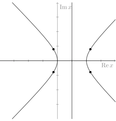
The solution set of the above equation is the union of the lines a = 1, b = 0 and the hyperbola a2₋₂_a₋_b2 _{= 0}_. _{The points}_x _{= 1}_±√₁_±₂_i _where_f₍_x_{) = 0 partition the set} Imf(x) = 0 into 5 components on which Ref(x) is either all positive or all negative (by continuity of f on the connected set Imf(x) = 0). See Figure 2.1 for a depiction of these components.

By plugging sample points from each component into f, we can determine the compo-nents on which f is negative. For example, we have

f(0) = 4, f(₋1_±i√3) =₋44,

(32)

Imx

Rex

Figure 2.1: The zero sets of Imf and f.

and so we see that f(x) < 0 exactly on the four components contained in the set B, i.e. along the branches of the hyperbola that lie outside the strip

Im1_±√1₋2i<Imx <Im1_±√1 + 2i.

For the purposes of constructing an appropriate cycle along which to integrate, we will only need the fact thatι1 and ι2 are holomorphic on the punctured strip

n

x_∈C_\0 : Im1_±√1₋2i<Imx <Im1_±√1 + 2io.

For the sake of completeness, however, we note that the details of Lemma 2.2.1 enable us to understand the global topology of_VQ as a Riemann surface. We take a moment to sketch

the construction.

(33)

Imx

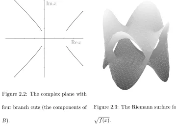
Rex

Figure 2.2: The complex plane with four branch cuts (the components of

B).

Figure 2.3: The Riemann surface for

p

f(x).

of the branch cut on the other, and vice versa.

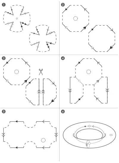
Similarly the Riemann surface for√x4_{+ 4}_x2₋₄_x3_{+ 4 can be constructed by beginning} with two copies of C_\B, i.e. two copies of the complex plane each with four branch cuts along which f(x) = x4_{+ 4}_x2 ₋₄_x3 _{+ 4} _≤ _{0. Local to the points} _x _{= 1}_±√₁_±₂_i _where

f(x) = 0, the Riemann surface forpf(x) should look like the Riemann surface for√x, and the branch cuts are glued together accordingly. Specifically, the tops of each of the branch cuts on one sheet are glued to the bottoms of the corresponding branch cuts on the other sheet, and vice versa. See Figure 2.2 for a representation of one of the sheets used in this construction, and Figure 2.3 for a depiction of the Riemann surface of pf(x).

The Riemann surface representation for_VQ is then the same as the Riemann surface for

p

(34)

torus with three puncture points. See Figure 2.4 on page 28 for a step-by-step construction demonstrating this fact.

Finally, as evidenced by Example 1.3.3, it will be useful for representing the residue form along_VQ to know whereQy = ∂Q_∂y is nonzero. Computing a Gr¨obner basis of the ideal

hQ, Qyi in Maple ([Wat08]) via the command

Basis([Q,diff(Q,y)],plex(y,x));

we obtain the univariate polynomial x4 + 4x2₋4x3+ 4 as the first basis element. Hence thexcoordinate of any point whereQandQy simultaneously vanish must be a root of this polynomial. This justifies the following remark.

Remark 2.2.2. AlongVQ, Qy is nonzero wheneverx6= 1±√1±2i(the roots of the equation

x4_{+ 4}_x2₋₄_x3_{+ 4 = 0).}

2.3 Representing the intersection cycle

The following lemma accounts for the first step of the analysis: using Corollary 1.3.7 to reduce the computation ofan,n to an integral onVQ.

Lemma 2.3.1. For ε >0, define

Cε={x∈C:|x|=ε},

the circle of radius ε about 0 _∈ C, oriented counterclockwise. Then for sufficiently small

ε >0,

an,n = 2πi

Z

ι1(Cε)

Res(ωF) + 2πi

Z

ι2(Cε)

(35)

2 1

4 3

6 5

Figure 2.4: A step-by-step construction starting with the two-sheeted representation ofVQ

(36)

Proof. We first verify that the variety _VQ is smooth. This is true only if Q, Qx and Qy do

not simultaneously vanish, which is true if and only if the varietyI =hQ, Qx, Qyiis trivial

(the whole polynomial ring). We check this algorithmically, using Gr¨obner bases. In Maple, we compute the Gr¨obner basis ofI with the command

Basis([Q,diff(Q,x),diff(Q,y)],plex(y,x));

Maple returns the basis[1] forI,so the ideal is indeed trivial. Now, let ε >0, δ >0 be sufficiently small so that

an,n=

Z

T0

ωF, whereT0={(x, y)∈C2 :|x|=ε,|y|=δ}

by Cauchy’s Integral Formula. Define the quantities

m0 = inf{|yj(x)|:x∈Cε, j = 1,2}, M0 = sup{|yj(x)|:x∈Cε, j= 1,2}.

For εsufficiently small, note that M0<∞ (by continuity of the yj; see Lemma 2.2.1) and m0 >0 (thex-axis intersectsVQ only at the point (2,0)).

Assume δ is chosen small enough so that δ < m0. Fix any M > M0.Then define the homotopy

K :T0×[0,1]→C2

(x, y, t)7→ x, y 1 +t M_δ −1

,

expandingT0in theydirection pastVQ.ThenKintersectsVQin the setC =ι1(Cε)∪ι2(Cε) and avoids the coordinate axes. Furthermore, K intersects _VQ transversely (as K expands

(37)

obtain

an,n= 2πi

Z

ι1(Cε)

Res(ωF) + 2πi

Z

ι2(Cε)

Res(ωF) +

Z

T1

ωF, (2.3.2)

where Cε is oriented counterclockwise (determined by examination of Theorem 1.2.2 and the Residue Theorem).

Now fixnlarge and letM vary. As the rest of the terms in (2.3.2) have noMdependence,

R

T1ωF must be a constant function ofM. But by trivial bounds, we can show that

Z

T1

ωF =O(M1−n) as M → ∞,

as ₍₂_πi₎P2_xyQ =O(1),exp(nH) =O(M−n) and the area ofT1isO(M).Forn >1, M1−n→0 asM _{→ ∞}.Hence the only constantR

T1ωF can be equal to is 0.

2.4 Saddle location and contour analysis

Step (2) in the analysis is to locate the saddle points ofh_|_V_Qand deform the contour of inte-gration appropriately, using this information. The saddle points can be found automatically as follows.

Lemma 2.4.1. h|VQ has three saddle points, located at

2,1₈

=ι1(2),

1−√5,3+₁₆√5=ι1(1− √

5),

1 +√5,3−₁₆√5=ι2(1 + √

5).

Proof. By Theorem 1.4.1, the critical points ofh_|_V_Qare those points whereQandxQx−yQy

(38)

Gr¨obner basis for the ideal I =_hQ, xQx−yQyi.This is done in Maple with the command

Basis([Q,x*diff(Q,x)-y*diff(Q,y)],plex(y,x));

which returns a basis consisting of the following two polynomials:

32₋8x2₋32x+ 20x3₋8x4+x5, x4₋48₋6x3+ 8x2+ 128y+ 16.

The first polynomial factors as (x2 ₋2x₋4)(x₋2)3,with roots x = 2 and x = 1_±√5.

Substituting these values ofxinto the second polynomial and solving foryyields the critical points claimed in the lemma.

We note here the interesting geometry near the critical point (2,1/8), which will turn out to be the sole contributing point. ExpandingH(ι1(x)) near x= 2,we obtain

H(ι1(x)) =H(ι1(2)) + 1

16(x−2)

4₊_O₍₍_x₋₂₎6₎_,

and hence h_|_V_Q has a degenerate saddle (of order 4) near this critical point, with steepest descent directions emanating fromx= 2 at angles π/4 +j(π/2) radians (j= 1,2,3,4.). We also see that along the path |x| = 2, h(ι1(x)) is locally minimized at x = 2, as this path passes through the critical point along ascent directions. Hence x= 2 is a local maximum for_|y1(x)|along this path, and so there are points (x, y)∈ VQnear (2,1/8) such that|x|= 2

and |y|<1/8.BecauseVQ cuts in toward the origin near ι1(2),this critical point is not on the boundary of the domain of convergence of F. In the terminology of the introduction, this critical point is not minimal.

(39)

Imx

Rex

p2

p3

p4

p5

p1

Figure 2.5: A pentagonal pathp. The dashed lines indicate the boundary of the punctured strip along which ι1 and ι2 are holomorphic.

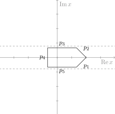
while the domain ι1(Cε) will be pushed to a “pentagonal” path through the critical point

(2,1/8).

The specific path to which ι1(Cε) will be deformed is ι1(p) where p is the pentagonal path depicted in Figure 2.5, with vertices at the points

₄

3 −i23,2,43 +i23,−23+i23,−23 −i23 . Denote by p1, . . . , p5 the edges of p,as denoted in the figure.

Performing the suggested deformation results in the following lemma.

Lemma 2.4.2.

an,n= 2πi

Z

ι1(p)

Res(ωF), (2.4.1)

(40)

Proof. For δ < ε, let K be a homotopy shrinking the circle Cε to the circle Cδ. By

holo-morphicity ofι2 (Lemma 2.2.1),ι2◦K is a homotopy fromι2(Cε) to ι2(Cδ) along VQ,and

Res(ωF) is holomorphic along this homotopy. By Stokes’ Theorem we obtain

Z

ι2(Cε)

Res(ωF) =

Z

ι2(Cδ)

Res(ωF).

Now fix n large and let δ vary. Note that as the left hand side of the above equation has no δ dependence, neither does the right.

By the fact that y2(x) = −4x−5(1 +O(x)) as x→ 0,we get that ₍₂_πi−₎2P_xyQy =O(δ−4), exp(nH) =O(δ4n_{) and the area of} _ι

2(Cδ) isO(δ−4) as δ →0.This implies that

Z

ι2(Cδ)

Res(ωF) =

Z

ι2(Cδ)

1 (2πi)2 ·

−P xyQy

enHdx=O(δ4n−8)

asδ_→0 (note that this representation of the residue is valid by Remark 2.2.2). For n >2, δ4n−8→0 as δ →0.Thus we must have that this integral is equal to 0.

As for the the integral over ι1(Cε) in (2.3.1), let K now be a homotopy expanding the

circleCεto the pentagonal pathp.Then by Lemma 2.2.1, ι1◦K is a homotopy fromι1(Cε)

toι2(p) along VQ,and Res(ωF) is likewise holomorphic along the image of this homotopy. Then by Stokes’ Theorem,

Z

ι1(Cε)

Res(ωF) =

Z

ι1(p)

Res(ωF),

wherep is oriented counterclockwise. The theorem follows.

(41)

Lemma 2.4.3. h(ι1(x))< h(ι1(2)) = log 4 ∀x∈p\ {2}.

Proof. Because h(ι1(x)) is continuous on the connected set p, we need only show that

h(ι1(x)) = log 4 for all6 x ∈ p\ {2}, and that h(ι1(x)) < log 4 for some x ∈ p\ {2}. The latter condition can be easily checked by plugging some arbitrary point into h(ι1(x)). As for the former condition, the idea will be to cook up some polynomial equations that must be satisfied in order for it to be true that h(ι1(x)) = log 4. We then use techniques from computational algebra to show that these equations can not be satisfied for any (x, y) with

x_∈p_{\ {}2_} and y=y1(x).

The conditions from which we will derive our polynomial equations are as follows:

1. x_∈pj for somej∈ {1, . . . ,5}.

2. y such that (x, y)_{∈ V}Q.

3. h(x, y) = log 4,oreh(x,y) = 4.

Each of these conditions implies a (set of) polynomial equations in the variables Re(x),

Im(x), Re(y) and Im(y), as we will show shortly. Note that we are throwing away some important information in condition 2 above, namely we wanty =y1(x),noty =y2(x).This will be important later in the proof.

We examine first the case where x∈ p3.Denote a= Re(x), b= Im(x), c= Re(y) and

d= Im(y).Then condition 1 implies the polynomial constraint:

P1 =b− 2 3 = 0.

(42)

Condition 2 implies the following two polynomial constraints:

P2= Re(Q(a+ib, c+id)) = 0,

P3= Im(Q(a+ib, c+id)) = 0.

Finally, condition 3 translates to 4_|x_||y_|= 1,or

P4= 16(a2+b2)(c2+d2)−1 = 0.

We are interested in whether these four polynomial equations have a commonreal-valued solution, and we will use Gr¨obner bases and Sturm sequences to answer this question. Since we expect the variety generated byI =_hP1, P2, P3, P4ito be finite —I is generated by four polynomials in four unknowns — we hope to use Gr¨obner bases to eliminate variables and produce a univariate polynomialB(a)_∈I.Any point (a, b, c, d) solvingPj = 0 for all j will

likewise solve B = 0. Then we try to use Sturm sequences to that such a B has no real rootsa∈[−2/3,4/3],proving that h(ι1(x))6= log 4 forx∈p3.

We compute the Gr¨obner basis with the command

Basis([P1,P2,P3,P4],plex(d,c,b,a))

and find that the first element B of the basis is univariate in the variablea, a polynomial of degree 16. We can check that B(₋2/3)₆= 0 and B(4/3)₆= 0 by direct computation in Maple. To check whether or not B has any roots on the interval (−2/3,4/3) we employ Sturm’s Theorem (see [BPR06, p. 52]).

(43)

Basis([B,diff(B,a)],plex(a));

returns the trivial basis [1], i.e. B is squarefree.

Then to count the number of roots in (₋2/3,4/3) via Sturm’s Theorem, we enter the command

sturm(sturmseq(B,a),a,-2/3,4/3)

and Maple returns that there are 0 real roots on the interval (₋2/3,4/3).

Computations are similar for p4 and p5,but things are a bit more complicated alongp1 and p2.Let’s look at p2.The first polynomial equation becomes

P1=a+b−2 = 0,

witha∈[4/3,2],while the rest of the polynomial equations remain the same. Going through the same procedure as before, we can produce a Gr¨obner basis for_hP1, P2, P3, P4i with an elementB(a) univariate ina. B(a) factors as

B(a) = (a₋2)4B˜(a),

where by direct computation we see that ˜B is nonzero at a = 4/3 and a = 2. Note: we expected thatB would have a root ata= 2,corresponding to the fact thath(ι1(2)) = log 4. The next step would be to attempt to show that ˜B has no roots on the interval (4/3,2),

but this is not true. Using Sturm sequences, one can show that ˜B has exactly one root

a0 ∈(4/3,2),and this is because there is a pair x, y withx∈p2\ {2}and h(x, y) = log 4. The claim is that this corresponds to a point where y=y2(x),not where y=y1(x).

(44)

continuous on p2\ {2}, there must be some x ∈ p2\ {2} such that h(ι2(x)) = log 4. This pair x, y=y2(x) satisfies the polynomial equationsPj = 0.

Now assume by way of contradiction thath(ι1(x)) = log 4 for somex∈p2\{2}.Because ˜

B has just one root a0 ∈(4/3,2),it must be that this occurs at the samex value for which

h(ι2(x)) = log 4,specifically x0 =a0+ (2−a0)i. Hence we have

|x0||y1(x0)|=|x0||y2(x0)|= 1 4,

which implies that _|y1|=|y2|at the pointx0.So at this value ofx we have

c2+d2 =_|y_|2=_|y1y2|= |

x₋2_| |x_|5

The preceding equation implies that _|x_|10(c2+d2)2 = _|x₋2_|2, which translates into the polynomial equation

P5 = (a2+b2)5(c2+d2)2−((a−2)2+b2) = 0.

We now have a new polynomial equation that must be satisfied in order to have that

h(ι1(x)) = log 4 on p2 \ {2}. But if we compute a Gr¨obner basis for hP1, . . . , P5i, we get the trivial basis [1], meaning that the polynomials have no common solution. Hence

h(ι1(x)) 6= log 4 for x ∈ p2 \ {2}. Analogous methods can be used to handle the case of

p1.

2.5 Saddle point integration

(45)

Theorem 2.5.1.

kn=an,n∼

4n 8Γ(3/4)n5/4.

Proof. We proceed from Lemma 2.4.2. The theorem will be proved in 2 steps: bounding the integral in (2.4.1) outside a neighborhood of the critical point, then applying saddle point techniques near that critical point.

For any neighborhoodN ofx= 2,we look atR

ι1(p\N)Res(ωF),which can be written as

Z

ι1(p\N) 1 (2πi)2 ·

−P xyQy

enHdx

(note that this representation is valid by Remark 2.2.2). As h _◦ι1 is continuous on the compact setp\N, h◦ι1 achieves an upper boundM onp\N.By Lemma 2.4.3,M <log 4. Thus by trivial bounds we have

Z

ι1(p\N)

Res(ωF) =O(eM n) =o((4−δ)n)

for sufficiently small δ >0,asn_{→ ∞}.Hence

an,n= 2πi

Z

ι1(p∩N)

Res(ωF) +o((4−δ)n). (2.5.1)

forany neighborhood N ofx= 2,providedδ is sufficiently small.

For N small enough, p ∩N = (p1 ∩N) ∪(p2 ∩N). We examine the integral over

ι1(p1∩N) andι1(p2∩N) separately, starting with ι1(p2∩N).By using the aforementioned representation of the residue form (and changing variables), we obtain

2πi

Z

ι1(p2∩N)

Res(ωF) =

Z

p2∩N 1 2πi·

−P(ι1(x))

xy1(x)Qy(ι1(x))

enH(ι1(x))dx.

After another change of variables (x_→x+ 2) and a suitable choice of neighborhoodN,the above integral can be rewritten as

4n

Z

γ+

(46)

where we have, for some fixedε >0,

γ(x) = (i₋1)x;x_∈[₋ε, ε], A(x) = 1

2πi·

−P(ι1(x+ 2))

(x+ 2)y1(x+ 2)Qy(ι1(x+ 2))

,

φ(x) = log 4−H(ι1(x+ 2)),

and we recall that γ+ is the restriction of the image of γ to the domain [0, ε]. The series expansion of Aand φatx= 0 begin

A(x) = i 16πx

3₊ i 32πx

4₊_O₍_x5₎_,

φ(x) = −1 16x

4₊_O₍_x6₎_,

and Reφ(x) is uniquely minimized onγ+atx= 0 where we haveφ(0) = 0,as a consequence of Lemma 2.4.3. Thus this is exactly the situation where the saddle point technique of Theorem 1.4.2 can be applied. The values ofbj andcj are as in the expansions above. Then v=γ′(0) =i−1,and we compute the principal root

(cknvk)1/k

v =

((−1/16)n(i−1)4)1/4

i₋1 =

−1−i

2√2 n 1/4_.

The conclusion of Theorem 1.4.2 is then

2πi

Z

ι1(p2∩N)

Res(ωF)∼4n − i

4πn−

1₊(1 +i) √

2Γ(5/4)

8π n−

5/4₊_O₍_n−3/2₎

!

As for the integral overι1(p1∩N),the same argument yields

2πi

Z

ι1(p1∩N)

Res(ωF) =−4n

Z

γ+

A(x)e−nφ(x)dx,

(47)

principal root

(cknvk)1/k

v =

((−1/16)n(−i−1)4)1/4 −i₋1 =

−1 +i

2√2 n 1/4_.

Then by Theorem 1.4.2 we obtain

2πi

Z

ι1(p1∩N)

Res(ωF)∼4n i

4πn−

1₊ (1−i) √

2Γ(5/4)

8π n−

5/4₊_O₍_n−3/2₎

!

.

Adding up the contribution over each piece and plugging into (2.5.1) yields

an,n ∼4n

√

2Γ(5/4) 4π n

−5/4₊_O₍_n−3/2₎

!

+o((4₋δ)n)_∼ 4

n√_2Γ(5_/₄₎

4π n

−5/4_.

(48)

Chapter 3

Homology of the Intersection Class

3.1 Setup and assumptions

We would like to produce an algorithm automating the analysis applied in the previous chap-ter. Tracing through the asymptotic analysis of bicolored supertrees, it becomes apparent that the main difficulty in realizing this goal will be achieving a sufficient understanding of the homology class of the intersection cycle. To obtain a homologous representative of the intersection cycle amenable to saddle point methods requires some global description of the singular variety – a potentially complicated space. Thus to begin, we must produce a description of the singular variety amenable to algorithmic study.

(49)

those points of sufficiently high (or low) value with respect to the height function, and the methods of Morse Theory reveal how the topology changes as regions of lower (or higher) height are unveiled. More details will be given in the following sections.

Portions of the following analysis will rely on topological properties of the bivariate case, and thus from here onward we will assume thatd= 2 variables. Hence the notation and the setup of the problem will be similar to that employed in the previous chapter. We write z = (x, y) rather than x = (x1, x2) to indicate points in C2. Similarly we write r= (r, s) =n(ˆr,sˆ) rather thanr= (r1, r2) =|r|(ˆr1,rˆ2).

We further impose the following assumptions on our analysis:

Assumption 3.1.1. Assume thatrˆand ˆsare positive rationals.

The preceding assumption is so that the points in Σ (the critical points of h on VQ)

can be found algorithmically using Gr¨obner bases. The additional assumption that ˆr and ˆ

s both be nonzero is to guarantee that this problem does not reduce to one of univariate rational asymptotics.

Assumption 3.1.2. Assume thatΣ is a finite set.

Note that the preceding assumption is generically true, but may fail for certain directions (ˆr,sˆ).

Assumption 3.1.3. Assume that_VQ is smooth.

Our analysis will apply under the preceding assumptions, with one last technical as-sumption to come later. Note that the asas-sumption that _VQ be smooth will be relaxed

(50)

3.2 Describing the variety at large height

Our Morse-theoretic analysis of _VQ begins with the selection of a suitable height function. For the singular variety VQ, we have the somewhat natural height function h=h(ˆr,sˆ), the function governing the exponential growth rate of the integrand from which we compute the asymptotics. Our first goal will be to describe what_VQ looks like for very large values of h. Consequently, we develop the following notation for better describing such sets.

Definition 3.2.1. For each constantM ∈Rwe define the set

V>M ={z∈ VQ:M < h(z)<∞}.

We define the sets _V≥M,_V<M and _V≤M similarly.

Note that implicit to the preceding definition is the fact that the variety_VQ is endowed

with a specific height function. Later, when we describe VQ relative to an auxiliary height

function, we will indicate this by modifying our notation for the variety itself.

We next wish to develop a description for _V>M for sufficiently largeM. By definition of

h we know that the height alongVQ is arbitrarily large only when|x|or|y|are sufficiently

small, so we first turn to understanding the variety near such points. We have the following useful characterization of a complex variety local to any xory value:

Theorem 3.2.2. LetB _⊆Cbe a circular neighborhood of x0 ∈Cslit along a ray emanating from x0. If the radius of B is sufficiently small, then on B every branch of Q(x, y) = 0 admits a representation y=f(x) of the form

f(x) = X

j≥j0

(51)

for a fixed determination of(x₋x0)1/k, where j0 ∈Z and k∈N. The function f is called a Puiseux expansion of y.

See [FS09, Theorem VII.7] for a proof, or [BK86] for a more in-depth discussion. Note that a similar result holds for obtaining the Puiseux expansion of x in terms ofy near any fixed value y=y0.

This local representation allows us to prove the following theorem.

Theorem 3.2.3. The set_VQ∩ {(x, y) : 0<|x|< R}, for sufficiently smallR, is diffeomor-phic to a finite set of disjoint, punctured open disks.

Each such diffeomorphism takes the form

G:U _−→D

z_7−→(zk, g(z))

for some integer k _≥ 1, where U is the punctured disk B_R1/k(0)− {0} and g is some

holomorphic function on U.

Proof. By Theorem 3.2.2, for x restricted to a small enough slit neighborhood of 0 in C, any branch of _VQ can be represented as (x, f(x)) for some fractional expansion

f(x) = X

j≥j0

cjxj/k.

We may assume thatf has been represented such thatkis as small as possible. Removing the slit,f can be extended to a neighborhood of the form

{x∈C:|x|< R, x6= 0}

(52)

Begin by defining the function

g(x) = X

j≥j0

cjxj,

a function holomorphic on the punctured diskU =B_R1/k(0)\ {0}. From this, we define the

function

G:U −→C2

z7−→(zk, g(z))

The goal is to show that G is actually a diffeomorphism between the punctured disk and the previously described branch, thus completing the theorem.

The first step is to show that Gis one-to-one, so begin by assuming that it is not. Then there arez16=z2 inU satisfying

zk₁ =zk₂ g(z1) =g(z2)

Denote z0 = z1k = zk2. This means that for two fixed determinations z1 and z2 of z01/k,

g(z1) = g(z2). Now we can write z2 =ξz1 for some kth root of unity ξ 6= 1. This means that

g(z1) =g(ξz1), and so

z₁mg(z1) =z1mg(ξz1),

where m = max (0,−j0). But the functions zmg(z) and zmg(ξz) are holomorphic on the diskB_R1/k(0) (multiplying byzm was done precisely to force holomorphicity atz= 0), and

(53)

1. The functionszm_g₍_z_{) and} _zm_g₍_ξz_{) agree on} _B

R1/k(0), or

2. By sufficiently minimizing the radiusR, we can assure thatzm_g₍_z_{) and}_zm_g₍_ξz_{) agree}

nowhere except possibly at the origin.

In the first case, it must be that the coefficients in the Taylor expansions of zmg(z) and

zmg(ξz) all agree, which means thatcj =cjξj for allj≥j0. Hencecj = 0 wheneverξj 6= 1. This means that cj 6= 0 only when j ∈sZ fors≥2 equal to the order of ξ, a divisor ofk.

But this implies that the fractional expansion f(x) can be written in terms of the (k/s)th rootsx(k/s), contradicting the minimality ofk. Thus we must be in the second case.

Hence by sufficiently minimizing the radius R for each possible kth _{root of unity} _ξ_{, we} can guarantee that the functionGis indeed one-to-one. The inverse functionG−1 is locally smooth because the functionz7→zk has a locally smooth inverse away from z= 0. Hence

G−1 _{is smooth, and so we see that} _G_{is indeed a diffeomorphism.}

Note that a similar result holds if we restrict to sufficiently small magnitudes ofyrather thanx. And furthermore, becauseQ(0)₆= 0 (asP/Qwas assumed to be holomorphic near 0 _∈ C), we can find a sufficiently small value of R so that no (x, y) ∈ VQ satisfies both

|x_| < R and _|y_| < R. The fact that these neighborhoods can be made disjoint will be important later on.

(54)

Assumption 3.2.4. By the Puiseux expansion, we know that we can parameterize each branch of VQ local tox= 0 in terms of x by writing

y=cxα(1 +o(1))

as x_→0 for some constants c₆= 0 andα. We assume that

α₆= −rˆ ˆ

s for all such branches.

Similarly, we can parameterize each branch of _VQ local to y= 0 in terms of y by writing

x=cyβ(1 +o(1))

as y_→0 for some constants c₆= 0 and β. We assume that

β₆= −sˆ ˆ

r for all such branches.

This assumption precludes us from taking asymptotics in only finitely many directions, as there are only finitely many branches of _VQ near x = 0 and y = 0. We also note that the finitely many possible values of α and β may be read from Newton polygon of the polynomial Q; see section 4.3 for further details.

The idea behind this assumption is to guarantee that h does not remain bounded as

x→0 and, necessarily,y→ ∞(or vice versa). This assumption is essential to the following lemma.

(55)

neighborhood, we can writey_∼cxα _as _x_→_{0, for some} _α_∈_Q _{and some constant} _c_{. Then,}

for sufficiently small R and any θ∈[0,2π], the function

hθ: (0, R]−→R

ρ_7−→h(ρeiθ, f(ρeiθ))

is monotone. That is, if the punctured disk is sufficiently small, the height function is monotone along rays emanating from the origin.

Furthermore, as ρ _→ 0, the height hθ approaches ∞ or −∞ according to whether α >

−ˆr/ˆsor α <₋r/ˆ sˆ, respectively.

Proof. Locally, thanks to the Puiseux expansion of y in terms of x, we can consider the functions H and h to be functions of a single complex variable. Namely

H(x) =₋ˆrlogx₋ˆslogf(x), and h(x) = ReH(x).

Then dhθ_dρ is simply the derivative ofh(x) with respect toρ, wherex=ρeiθ. As h= ReH,

this can be represented as

dhθ dρ =

RedH

dx

cosθ−

ImdH

dx

sinθ

x=ρeiθ

So we turn to evaluating dH_dx.