A NEURAL NETWORK MODEL FOR
SHORT TERM PREDICTION OF
SURFACE OZONE AT TROPICAL CITY
R.SAMUEL SELVARAJDepartment of Physics, Presidency College, Chennai – 600 005, India. K. ELAMPARI1
Research Department of Physics, S.T. Hindu College, Nagercoil – 629 002, India. R. GAYATHRI
Dhanalakshmi Srinivasan College of Engineering and Technology, Mamallapuram, Chennai,India. S. JOHNSON JEYAKUMAR
Department of Physics, TBML College, Porayar – 609 307, India. Abstract:
A new method for short term prediction is presented using the neural network technique. Due to increase in industrial and anthropogenic activity, air pollution is a serious subject of concern today. Surface ozone prediction using the technique of adaptive pattern recognition is developed. The model can predict the mean surface ozone based on the parameters like Nitrogen-di-oxide, temperature and % Relative Humidity. The model can perform well both in training and independent periods. The classical methods of short term modeling are not reliable enough. The method can also be used for short term prediction of other air pollutants.
Key words: Air pollution; Neural network; Surface ozone; Short term prediction.
1. Introduction
Surface ozone is a secondary photochemical pollutant produced from a variety of natural and anthropogenic precursors that include industrial and vehicular emission of volatile organic compounds and oxides of nitrogen. In elevated concentrations, it has detrimental effects on vegetation, human health and various natural materials [Guicherit et al., (1987)]. Ozone is an important constituent of the atmosphere that maintains the thermal structure of the stratosphere and the troposphere. Many studies [Ramaswamy and Bowen, (1994); Rajeevan, (1996); Bojkov, (1983)] suggest that an increase in tropospheric ozone leads to the warming in surface temperature. Ozone is considered to be the cause of eye irritation and may affect the respiratory tract [Amdt, (1980)] even during short term high concentrations.
The non-linear relationship of surface ozone with solar radiation has been mentioned by Bravo et al. (1996). There is a value of solar radiation for which ozone concentration has a maximum. This effect may be due to days with high solar flux having little atmospheric pollution, with little ozone formation and high atmospheric transparency [Bravo et al., (1996)]. The problem of short term modeling in complex terrain are discussed in details by Bonzar et al. (1993). They have also shown that in the case of stable atmosphere and of thermal inversions the failure of dispersion model and the inadequacy of this model for controlling emissions. In this regard they have applied the neural network technique for short term prediction. The results obtained by them are significantly better than those obtained from conventional models.
1
Neural network techniques have recently become the focus of much attention as they can handle the complex and non-linear problems better than the conventional statistical techniques. Neural network is simple mathematical input output model which learns the relationship (linear or non-linear) between the input and output during the training period. Neural network model brings out the maximum information available within the data during the training period and reflects these in the independent period. Present paper aims to develop a simple model using neural network technique based on the data which are easily available. The performance of the model is satisfactory both in training and independent period.
2. Area of Study and data
The study area Chenbagaramanputhur (8o15’1”N, 77o29’19”E) is a rural place in Kanyakumari district and is about 12 km from Nagercoil town.
The following parameters were used to develop the model: (1) Mean surface ozone concentration as response. (2) Nitrogen dioxide concentration as predictor. (3) Mean temperature as predictor.
(4) Prevailing % Relative Humidity as predictor.
3. Method of data measurement
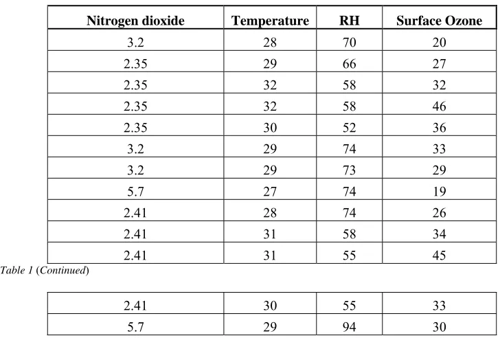
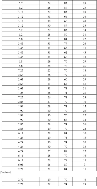
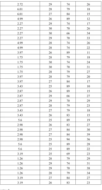
Ground level ozone concentration and nitrogen dioxide measurements were carried out in the rural site Chebagaramanputhur. A portable Aeroqual series S200 ozone monitor was used. An Aeroqual series S200 ozone monitor is constructed to measure low and high ozone levels. Its ultra low concentration ozone head measures the ozone concentration from 0.000 to 0.500 ppm, and a high concentration ozone head measures the ozone concentration from 0.50 to 20.00 ppm. Accuracy of a low concentration ozone head is +/- 0.001 ppm (from 0 to 0.100 ppm); +/- 10% (0.100 to 0.500 ppm), while that of a high concentration ozone head is +/- 10% (from 0.20 to 2.00 ppm); +/- 15% (from 2.00 to 20.00 ppm), the measurement unit being either ppm or μg/m3. The operating temperature range is from – 5o C to 50o C, relative humidity limits are 5% and 95%. Similar kind of NO2 sensor has been used for nitrogen dioxide measurement. A gas sensitive semiconductor (GSS) type sensor is described in www.aeroqual.com. Sampling was carried out for three months from May 2009 to July 2009. For ozone seven readings were taken per day starting from 0530h to 2330h with 3 hour interval. For NO2 only two readings were taken one at daytime and the other at nighttime. The data obtained is tabulated in Table 1.
Table 1. Predictor parameters with ozone values observed
Nitrogen dioxide Temperature RH Surface Ozone
3.2 28 70 20
2.35 29 66 27
2.35 32 58 32
2.35 32 58 46
2.35 30 52 36
3.2 29 74 33
3.2 29 73 29
5.7 27 74 19
2.41 28 74 26
2.41 31 58 34
2.41 31 55 45
Table 1 (Continued)
2.41 30 55 33
5.7 29 83 28
6.2 28 89 23
3.12 29 83 28
3.12 31 66 36
3.12 30 66 48
3.12 30 89 35
6.2 29 83 34
6.2 28 80 31
6.8 27 84 22
3.45 31 79 26
3.45 31 62 31
3.45 31 62 43
3.45 31 66 33
6.8 29 70 29
6.8 28 76 26
7.25 25 70 18
2.63 26 79 25
2.63 29 60 29
2.63 31 62 41
2.63 31 74 31
7.25 26 74 25
7.25 26 74 23
2.85 27 79 10
1.99 29 74 15
1.99 30 70 29
1.99 30 70 32
1.99 30 66 32
2.85 29 74 26
2.85 29 70 24
6.11 28 84 10
4.24 29 74 15
4.24 30 74 20
4.24 30 70 33
4.24 27 89 27
6.11 28 79 16
6.11 28 79 15
6.01 26 89 7
2.72 28 84 11
Table 1 (Continued)
2.72 29 79 16
2.72 29 74 26
6.01 28 79 18
6.01 27 84 15
4.99 26 89 12
2.27 29 74 17
2.27 30 70 26
2.27 30 66 34
2.27 29 70 33
4.99 28 74 26
4.99 28 74 22
3.97 26 89 11
1.75 28 79 18
1.75 30 74 24
1.75 30 70 31
1.75 28 79 27
3.97 28 79 20
3.97 27 84 17
3.43 25 89 10
2.87 26 89 15
2.87 29 66 27
2.87 29 70 29
2.87 28 79 23
3.43 27 79 18
3.43 26 83 15
5.6 25 89 19
2.98 26 83 27
2.98 27 84 30
2.98 27 84 39
2.98 25 94 36
5.6 25 89 28
5.6 25 89 22
3.19 25 69 23
1.26 28 79 29
1.26 29 74 31
1.26 29 70 38
1.26 28 79 34
3.19 27 84 27
3.19 26 83 23
Table 1 (Continued)
3.15 27 73 15
3.15 29 74 27
3.15 29 74 32
3.15 28 79 30
6.93 27 84 24
6.93 26 83 21
7.47 27 84 24
3.42 29 74 27
3.42 29 100 30
3.42 29 74 34
3.42 28 79 34
7.47 28 84 27
7.47 27 84 23
3.62 26 89 17
2.87 26 89 20
2.87 29 74 30
2.87 28 79 40
2.87 29 74 34
3.62 27 84 29
3.62 27 84 25
1.79 26 89 23
1.42 29 74 25
1.42 29 74 32
1.42 28 79 37
1.42 28 79 38
1.79 28 79 32
1.79 27 84 28
4. Brief review of neural network technique
Neural Networks are signal processing systems that attempt to emulate the behavior of biological nervous systems by providing a mathematical model of combination of numerous basic blocks called neurons connected in a network. It is remotely analogous to living nervous system and hence its name. One can think of neural networks as an extended form of regression which has the properties of
(1) adaptivity (2) robustness, (3) ruggedness,
(4) speed (via massive parallelism), (5) nonlinearity and
(6) optimality with respect to error.
training sets, after the learning process, the trained network is capable of predicting the ozone concentrations as an output according to the inputs and internal structure of the network established during the learning period.
The most common neural network is the feedforward mapping network, it consists of a set of nodes and a set of interconnections between them. A node contains a computational element called neuron , taking inputs from incoming interconnections (input links) and providing outputs to outgoing interconnections (output links). The units of the neural network are arranged by layers. A unit on one layer takes inputs from the units on the layers below and feeds its output to the units on the layers above. The bottom layer is called input layer whose units take input from the outside and without processing them distribute to the units on the layer above. The top layer is an output layer whose output is the output of the neural network. The layers between input and output layers are called hidden layers. A pattern is defined as a set of input values with the related output values. A typical computational element takes the weighted sum of the input links and passes the result through a transfer function.
The structure of a three layer neural network is shown in Fig. 1. The transfer function used here is the sigmoidal function.
Y = [1 + e (-ax+b)]-1 (1)
Where ‘a’ determines the slope of the sigmoid and ‘b’ is the threshold. The process of learning the training set of patterns means the determination of the optimum weights which minimize the mean square error between the outputs in the output layer and the desired values. Most commonly used “back-propagation learning algorithm” [Rumbelhart et al., (1986)] is used for the training. Initially random weights between ±0.5 are assigned to each weight as initial guesses. The weights are learned through an iterative process. During learning the weights are updated.
When the network learns the training set of patterns well enough it can be used for determining the output values for the pattern with unknown outputs (Test period or prediction period).
Fig.1 : Three layer architecture proposed
5. Results and conclusions
Fig.2 Surface ozone - Predicted versus Actual values
The mean square error of the data during testing is 0.15375 ppb.
The accuracy of testing data is 99.85 %.
The above results validate the proposed model. Hence it is concluded that the above model can be used for predicting surface ozone concentration with nitrogen dioxide, temperature, % relative humidity as predictors.
References
[1] Amdt, U. (1980): Wirkungsaspekte im Hindblick auf die Grenzwertziehung von ozone, In photochemische Luftverunreinigungen in der
Bundesrepublik Deutschland, Tagung des Umweltbundesamtes, Oct, 1979, VDI – Verlag, Dusseldorf, pp. 229 – 238.
[2] Bojkov, R.D. (1983): Tropospheric ozone, its changes and possible radiative effects, Proc. WMO Techn. Conf. on Observ. Of Atmosph.
Contamin. Vienna, Oct. 1983. WMO Sp. Environm. Report 16.
[3] Bonzar, M.; Lesjak, M .; Mlakar, P. (1993): A neural network based method for short term predictions of ambient SO2 concentration in
highly polluted industrial areas of complex terrain. Atmospheric Environment, Part B: Urban Atmosphere, 27B, 2, 221-230.
[4] Bravo,J.L.; Diaz, M.T.; Gay, C ; Fajardo, J. (1996):A short term prediction model for surface ozone at southwest part of Mexico valley,
Atmosfera, 9, 33-45.
[5] Guicherit, R. et.al., (1987):The regional ozone problem in Tropospheric ozone – Regional and Global Scale interactions, Nato ASI Series
C. 227 (1988), 403-411.
[6] Masters, T., (1993): Practical Neural Network Recipies in C++, Academic Press.
[7] Rajeevan, M. (1996): Climate implications of observed changes in ozone vertical distribution, Int. J. Climatol., 6, 15-22.
[8] Ramaswamy, V.; Bowen, M.M. (1994): Effect of changes in radiatively active species upon lower stratospheric temperatures, J. Geophys. Res.,99, 18909-18921.
[9] Rumbelhart, D.; Hinton, G.E.; Wiliams, R.J. (1986): Learning internal representation by error propagation, In parallel distributed processing Exploration in the Microstructure of Cognition, Vol I, Cambridge.
0 10 20 30 40 50
1 4 7 10 13 16 19 22 25 28
Surface
ozone
in
ppb
‐
‐
>
Performance
of
ANN
on
training
data
Predicted