Ruiting Yang. Predicting the Popularity of TED Talks. A Master’s Paper for the M.S. in I.S degree. May, 2020. 63 pages. Advisor: Yue Wang
In this paper, we explore how to predict a TED talk’s popularity by its inherent features via machine learning techniques. We quantify a TED talk’s popularity as logarithmic transformation of its daily views and daily comments and include 43 features as predictors. We find that the ordinary least squares regression, ridge regression, and LASSO regression models perform well, and predictors such as a talk’s number of language translations, average Internet development environment when published, duration, main speaker’s occupation, as well as the timing it being uploaded have essential effects on its popularity. In the end, we also provide our suggestion on how to improve TED talks’ popularity within and beyond the scope of machine learning.
All the materials in this research (including but not limited to original and processed data, figures, tables, etc.) are under the Creative Commons License: BY-NC-ND 3.01.
Headings:
TED talks popularity
Machine learning
Linear regression
Ordinary least squares (OLS)
Best feature subset
Ridge regression
LASSO regression
PREDICTING THE POPULARITY OF TED TALKS
by Ruiting Yang
A Master’s paper submitted to the faculty of the School of Information and Library Science of the University of North Carolina at Chapel Hill
in partial fulfillment of the requirements for the degree of Master of Science in
Information Science.
Chapel Hill, North Carolina
May 2020
Approved by
CONTENTS
Introduction ... 2
Literature Review ... 6
How to Quantify “Popularity” ... 6
Possible Predictors for “Popularity” ... 8
Applicable Machine Learning Methods ... 9
Evaluation Metrics ... 11
Problem Statement and Data Description ... 13
Problem Statement ... 13
How the Original Dataset is Preprocessed ... 15
Dependent Variables ... 16
Independent Variables ... 19
Preprocessed Data’s Statistics ... 24
Method ... 27
Training, Validation and Test Datasets ... 27
Machine Learning Models ... 28
Linear Regression ... 28
Random Forest ... 31
Result ... 32
Prediction Performance ... 32
Linear Regression ... 32
Random Forest ... 37
Learned Parameter Importance ... 39
Linear Regression ... 39
Random Forest ... 44
Discussion ... 48
What Machine Learning Prediction Can Tell us ... 48
What Machine Learning Prediction Cannot Tell us ... 49
Conclusion ... 51
Note ... 52
Introduction
Founded by Richard Saul Wurman in 1984 as a conference and under the slogan “ideas
worth spreading” (“TED (conference)”2, 2020), TED is one of the most well-known
non-profit organizations in the world for its powerful impact on education. Based on the data
from TED talks3, since June 2006, when TED released its first talk for free viewing
online, TED has offered more than 3,300 talks covering various topics from science to
humanities to daily lives in over 110 languages as of March 2020. According to TED
Blog4, TED surpassed a billion video views in total back to November 2012. Also based
on the data from TED talks5, until March 2020, the most popular talk on TED has gained
over 64 million views, and the median views of all the talks have also reached 1.2
million.
It is not surprising to acknowledge that TED Talk, an online educational platform
devoted to spreading ideas, has valued and will be valuing the popularity of its content
(web-based talks) all the time. As Pinto, Almeida, & Gonçalves (2013) points out, “web
content popularity is of great importance to support and drive the design and management
of various services.” In TED’s case, “various services” are reflected on its slogan “ideas
worth spreading” including producing high-quality videos, finding sponsorship from
partnerships, establishing TED Fellows programs to support new voices, etc. (How TED
Additionally, from the audience’s perspective, a higher level of video popularity means
more chances to be exposed to TED talks, especially for people who are willing to learn
via online platforms at the age of social media. More chances of being exposed to
cutting-edge and high-quality ideas like TED provides, more times of educational
inspiration could be expected to happen.
What is more, given educational communities, TED’s success in collecting brilliant ideas
from all over the world and spreading them further and further could function as a
prototype model for people in the field of education generating and spreading
high-quality content. Wingrove (2017)’s research also reveals that “TED talk variation enables
a range of academic listening applications.” To learn from TED’s successful experiences
in education, the reasons for the TED talk’s popularity is also worth exploring.
Then, how can we approach the myth behind TED talks’ popularity from the aspect of
information science? Machine learning is an ideal solution. Murphy (2012) defines
machine learning as “a set of methods that can automatically detect patterns in data, and
then use the uncovered patterns to predict future data, or to perform other kinds of
decision making under uncertainty.”
In this paper, we will “detect patterns,” “predict future data,” and “perform decision
making” (Murphy, 2012) via machine learning methods of linear regression and random
forest in terms of the data related to TED talks’ popularity. Relying on the dataset
Pappas and Popescu-Belis (2013)’s work, we quantify a TED talk’s popularity as log of
its daily views and log of daily comments and include 43 TED inherent features as
predictors for a talk’s popularity. We find that OLS, Ridge, and LASSO models perform
well in our prediction, and features such as the number of language translations, average
Internet connection speed, duration, posting gap between the date of being filmed and the
date of being published, main speaker’s occupation as writer or psychologist, being
themed on “culture” or “design”, being published on Friday, Saturday or March are all
powerful predictors.
In summary, this paper focuses on predicting a TED talk’s popularity by its features
using machine learning techniques. Given the historical data retrieved and the machine
learning models such as linear regression and random forest, this research is promising in
practice. Also, it is worth-pursuing in theory since figuring out what makes a TED talk
popular is of great value for TED, TED’s audience, the general public who are willing to
learn through video-hosting platforms, existing and potential educators, educational
communities, and even the social literacy environment.
The paper proceeds as follows. The literature review section focuses on having an
overview of the research background. The problem statement and data description section
states our research goal and how we process the raw data to generate dependent and
independent variables. The method section introduces our rationale for using linear
regression and random forest models. The result section displays different models’
findings based on as well as beyond the scope of machine learning prediction. Finally, the
conclusion section summarizes all the work we have done in this research and looks into
Literature Review
We will review relevant literature of our research to have an overview of the research
background from four perspectives: how to quantify “popularity,” possible predictors for
“popularity,” applicable machine learning methods, and evaluation metrics.
How to Quantify “Popularity”
Since the dataset on Kaggle8 has been as open source for anyone since published in 2017
September, there have been many practices with the same topic of mine, and they offer
me a robust and practical platform to quantify a TED talk’s popularity. Based on the
same dataset that I intend to use, explored indicators that can represent a TED talk’s
popularity include and don’t limit to:
1. the number of views (Alvarez, 2017; Banik, 2017; Eldor, 2018; Kumar, 2017);
2. the number of comments, which is assumed as a reflection of “constructive
criticism” and online community involvement (Banik, 2017);
3. the ratio of positive to negative ratings (Yuen, 2018).
These three indicators have also been further discussed. For instance, similar to the
concept of “popularity,” Moser (2017) defined how “powerful” a TED talk’s idea is by
combining three features: the number of views, the number of positive ratings, and the
and the number of comments were correlated.” Tanveer et al. (2019)’s research
mentioned that “the longer a TED talk remains on the web, the more views it gets,”
which means the “age” of a talk should be considered into the change of its number of
views.
Not limited to the existing dataset, the general idea behind our research topic is based on
what evidence can we reveal a underlying web-based content’s attribute, which, in my
case, is “popularity.” Therefore, we also broaden our horizon for reviewing outside
research regarding different types of web-contents’ popularity. Some good examples in
point are Liu et al. (2017) used audience’s applause as an indicator of user engagement
based on analyzing TED talks’ transcripts; Chen and Lee (2017) predicted humorous
utterances using audience’s laughter based on TED talks; Chen et al. (2016) focused on
predicting the popularity of micro-videos on Vine using four indicators: the number of
comments, the number of likes, the number of reposts and the number of views; Hong et
al. (2011) targeted on Twitter and measured a tweet’s popularity by the number of its
future retweets; Cappallo et al. (2015) defined an image’s popularity by its view count
and the number of comments, etc. Besides, not surprisingly, on top of common popularity
prediction for videos, social media, and images, almost every kind of web content’s
popularity has been measured for exploration, such as online news (Fernandes et al.,
2015), even for Github repositories (Borges, 2016).
To sum up, based on prior experience, we have learned that almost every type of web
interaction with it, which in the TED talk’s case could be the number of views or the
number of comments. At the same time, we take the “accumulating effect” into account,
given a longer time of an item remaining online naturally triggers more human
interactions with it. Therefore, we think it would be more reasonable to use the number of
averaged views or comments of each TED talk in a certain period as the indicator of their
popularity.
Possible Predictors for “Popularity”
Given “popularity,” what are the possible predictors for it? In other words, what
features/attributes/characteristics of a TED talk can we use to predict its popularity? In
this sense, explored features in the previous work that can be applied to our research are a
TED talk’s:
1. marked theme(s) (Alvarez, 2017; Banik, 2017; Yuen, 2018)
2. number of the marked tag(s) (Eldor, 2018)
3. year of the published date (Alvarez, 2017; Banik, 2017; Kumar, 2017)
4. duration of the talk (Alvarez, 2017; Banik, 2017; Kumar, 2017)
5. days between video creation and publishing (Alvarez, 2017)
6. days between publishing and dataset collection (Alvarez, 2017)
7. translations in languages (Eldor, 2018; Banik, 2017)
8. being published on what day of a week (Eldor, 2018; Banik, 2017; Yuen, 2018)
9. being published on which month of a year (Banik, 2017; Kumar, 2017)
10. speaker’s occupation(s) (Eldor, 2018; Banik, 2017; Kumar, 2017; Yuen, 2018)
12. word count (Banik, 2017)
13. voted count of “variety of metrics” like “funny,” “inspiring”… (Banik, 2017)
14. length of video description (Kumar, 2017)
15. belonging to which TED event (e.g., TEDx) (Banik, 2017; Kumar, 2017)
16. whether occurring in the popular words’ cloud created by all talks’ titles or
description (Banik, 2017; Yuen, 2018)
Our research will rely on these features to find the most successful predictors
combination among them, which achieves the best performance on predicting a TED
talk’s popularity.
Applicable Machine Learning Methods
Based on the summary of machine learning by Ray (2017), one type is called supervised
learning which refers to “algorithm consisting of a target/outcome variable (or dependent
variable) which is to be predicted from a given set of predictors (independent variables).”
(Ray, 2017); and the other type is called unsupervised learning which means “in this
algorithm, we do not have any target or outcome variable to predict or estimate.” (Ray,
2017). In our case, since we do have a target variable, which is a TED talk’s popularity,
we will be using supervised machine learning models.
In terms of supervised machine learning models, Provost & Fawcett (2013) and Ray
(2017) both bring up linear regression, logistic regression, decision trees, support vector
well as neural networks. And most of these machine learning models have been tried, and
therefore, they can be regarded as applicable. The detailed applications are as follows:
From the perspective of linear regression, it has been used to predict YouTube video’s
popularity (Ma, Yan, & Chen, 2017; Pinto, Almeida, & Gonçalves, 2013), TED talk’s
applause, another indicator of TED popularity as mentioned (Liu et al., 2017), how
suitable TED talks are for academic listening (Wingrove, 2017), the popularity of GitHub
repositories (Borges, Hora, & Valente, 2016). In terms of logistic regression and decision
trees, Ray, Yadav, & Garg (2018) ’s work used both to conduct a predictive analysis
using classification algorithms on TED Talks. For support vector machines (SVM),
successful applications are predicting the popularity of online videos (Trzciński and
Rokita, 2017), the popularity of social media (Hidayati et al., 2017), the
popularity of social image (Huang et al., 2017). Given naive Bayes, there are social
content popularity prediction conducted by Wu et al. (2018). In the case of k-nearest
neighbor algorithm (KNN) and random forest, Ray, Yadav & Garg’s work (2018) again
employed both techniques. Besides, the random forest model has been applied to
predicting the popularity of TED talks by Dochev (2019) as well as online news by
Fernandes, Vinagre, & Cortez (2015). Last but not least, concerning neural networks,
TED Talk ratings have been predicted from language and prosody through this method
by Tanveer et al. (2019). So has the audience’s laughter via Convolutional Neural
Network (CNN) by Chen & Lee (2017). Plus, also based on the popularity prediction of
streaming service, Jeon et al. (2019) focused on the newly released contents for online
We decide to employ both linear regression and random forest models for our research
since they are classical in practical experiments so that they can further compare and
mutually prove each other’s findings.
Evaluation Metrics
An integral part of machine learning is doing the evaluation. In our research’s case, the
evaluation question would be, how can we decide whether a model with certain features
outperform the other one? Provost & Fawcett (2013) have mentioned various evaluation
metrics for machine learning models under various assumptions, such as “mean squared
error”, “accuracy”, “precision”, “recall”, “F1 score”, “ROC curve”, “confusion matrix”...
It is never easy to choose from them, while with the help of relevant literature, things
could also get a little easier since there are successful cases to learn from. Specifically
speaking, a fit evaluation metric is mainly determined by the dependent variable. If the
dependent variable is “number of views” or “number of comments,” then it’s a numerical
prediction task. In that case, “mean squared error” or “mean absolute error” can be used
(e.g., Dochev, 2019, etc.). If the dependent variable is “whether the number of views is
above 100k” (true or false, binary classification), or “the number of reviews is 0-100k,
100k-1M, or 1M” (three-way classification), then we will need to use an evaluation
metric for classification, in which case (e.g., Yuen, 2018, etc.), “accuracy”, “precision”,
Given our dataset supports us in conducting predictions on a numerical dependent
variable, mean squared error (MSE) or mean absolute error (MAE) will be the primary
Problem Statement and Data Description
In this section, we will start by stating the research problem. Then, based on the research
problem, we will describe the original dataset, illustrate how we preprocessed it for
further data exploration, and show the preprocessed data statistics.
Problem Statement
Our research problem is to predict the popularity of a TED talk given its inherent
attributes using machine learning techniques.
Given “popularity”, we will find numerical indicators such as a TED talk’s daily views
and daily comments to represent this information.
In terms of “inherent attributes”, we mean the attributes that are generated on or before
the time when a TED talk is uploaded online. For example, a TED talk’s title length,
duration, published on what day of a week, speaker(s)’ occupation(s), related tags,
number of translated languages, etc. We decide to only focus on these “inherent
attributes” since we would like to carry out our prediction as soon as a TED talk is
published. In other words, we will not consider the features that will emerge only after a
For “machine learning techniques”, we will focus on linear regressions and random
forest.
The Original Dataset
The original dataset on Kaggle9 contains all 2,550 TED talks published on the official
TED.com website from February 24th, 2006 to September 22nd, 2017.
For each TED talk in the original dataset, captured features include a talk’s title,
description (a summary of what the talk is about), main speaker (the first-named speaker
of the talk), main speaker’s occupation, number of speakers, the duration of the talk in
seconds, in which event the talk took place, the Unix timestamp of the filming date, the
Unix timestamp for the publication date, the tags/themes associated with the talk, the
number of language translations, ratings (e.g., a talk can be rated by voting from various
dimensions and stored as {'name': 'Funny', 'count': 19645}, {''name': 'Beautiful', 'count':
4573}…), a list of talks recommended for continuing to watch, the URL link, number of
comments, and number of views.
To conduct further data exploration for our research, figuring out the original data’s data
types matters as they determine how the data preprocessing would be. Generally
speaking, there are four data types: categorical, ordinal, interval, and ratio/proportional.
According to O'Sullivan, et al. (2016), “categorical variables are measured with nominal
scales—identifying and labeling categories...do not have a relative value.” In the case of
data from the original dataset, categorical data include a talk’s title, description, main
speaker’s occupation, in which event the talk took place, the tags/themes associated with
the talk, ratings, a list of talks recommended for continuing to watch, and the URL link.
Ordinal variables “identify and categorize values of a variable and put them in rank order
according to those values… without regard to the distance between values” (O'Sulliva, et
al., 2016). Given this dataset, there are no ordinal data.
“Interval and ratio scales measure characteristics by ranking their values on a scale and
determining the numerical differences between them” (O'Sulliva, et al., 2016). And “a
ratio scale has an absolute zero; an interval scale does not” (O'Sulliva, et al., 2016).
Therefore, the interval data include a talk’s Unix timestamp of the filming date, Unix
timestamp for the publication date. And the ratio data include the number of speakers, the
duration of the talk in seconds, the number of language translations, number of
comments, and number of views.
How the Original Dataset is Preprocessed
As we are attempting to figure out the effect of various TED talk attributes on a TED
talk’s popularity, the dependent variable is TED talk’s popularity, and the independent
will further demonstrate how the original dataset is preprocessed from the perspectives of
these two types of variables.
Dependent Variables
In terms of the dependent variable, “popularity,” we decide to use: daily views of a TED
talk, as well as daily comments of a TED talk as two separate indicators. In other words,
we will run the same models with the same set of independent variables twice based on
two different dependent variables.
Both dependent variables can be calculated by the total number of views or comments
divided by the number of days gap between the date when a talk was published and the
date when the dataset was collected (September 25th, 2017).
The reason for making this decision is aligned with the findings from the literature
review. In essence, we believe the natural time effect on accumulating a TED talk’s
views or comments so that we are averaging it out. Also, we deem “views” and
“comments” could reflect different aspects of “popularity” so that we should separate
them, for instance, more views can be regarded as more times of a video being clicked,
while more comments usually mean more discussion is inspired.
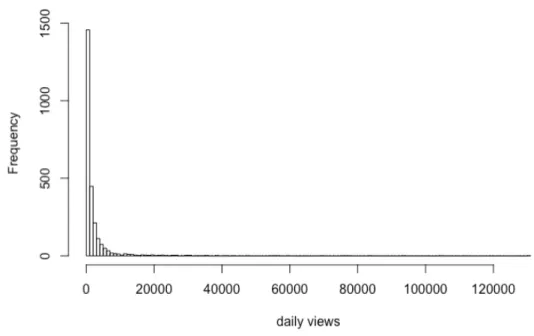
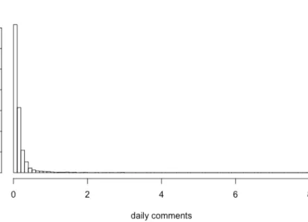
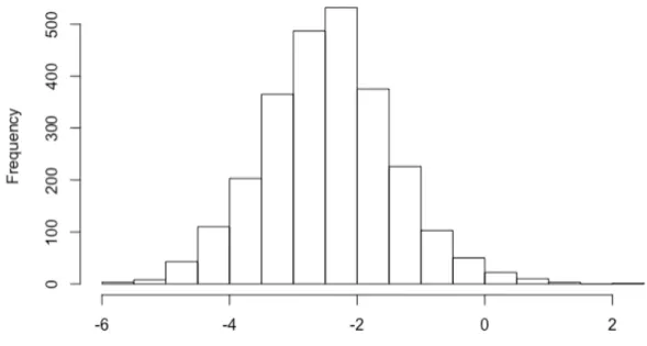
Also, we plotted these two variables (as shown in Figure 1 and Figure 2) given all 2,550
talks’ distribution frequency, and we found that both of their patterns are highly right-
dependent variables, we conducted natural logarithmic transformations on both of them
and found that their log-transformed values’ patterns both approximate the normal
distribution (as shown in Figure 3 and Figure 4) and are more suitable given machine
learning model construction. Therefore, we decide to use the logarithm of both variables
as our two dependent variables:
1. log of daily views
2. log of daily comments
Figure 2. Distribution of daily comments for all 2,550 talks
Figure 4. Distribution of log(daily comments) for all 2,550 talks
Independent Variables
Concerning independent variables, also based on the literature review, almost every
captured feature mentioned can be deemed as an independent variable, while the
variables that can be directly used are only:
1. number of language translations;
Other ones are all in need of being further engineered more or less. For example, the
published date and filmed date need to be converted to standard date format so that we
could calculate the number of days difference between them as a variable:
3. posting gap;
Given the posting gap, we found 9 abnormal talks – each of them shows a negative value.
We tracked them back on the TED website and we believe it is because their published
dates are wrongly recorded on the website. Therefore, we removed these 9 talks, and the
full size of our dataset drops to 2,541.
For easier interpretation, we also convert duration in seconds to:
4. duration in minutes;
Besides, to measure the length of a talk’s title by how many characters it owns, we create
a variable:
5. title length;
Additionally, we introduce an outside-sourced feature:
6. mbp;
This feature, “mbp,” represents U.S. average internet connection speed in Mbps (million
bits transferred per second). This data is originally collected by Akamai Technologies10
every quarter (Q) from 2007 Q3 to 2017 Q1 and further organized by Statista11. We
intentionally add this feature to the model building, since we believe the development of
popular, and this feature can be a good indicator for the blurred concept, “Internet
development”. Additionally, since the original data source only captured “mbp” from
2007 Q3 to 2017 Q1, while the published date of all 2,541 talks ranges from 2006 Q2 to
2017 Q3, we approximated and filled 7 missing “mbp” values holding the assumption
that the increasing rate of “mbp” between two quarters is same as the averaged increasing
rate of “mbp” among their closest five quarters with known values.
Plus, to capture the information of what day on a week might affect a talk’s popularity,
we create many dummy variables, for instance:
7. Mon (using 1 or 0 to represent a talk is published on Monday or not);
8. Tue (using 1 or 0 to represent a talk is published on Tuesday or not);
9. Wed (using 1 or 0 to represent a talk is published on Wednesday not);
10.Thur (using 1 or 0 to represent a talk is published on Thursday or not);
11. Fri (using 1 or 0 to represent a talk is published on Friday or not);
12. Sat (using 1 or 0 to represent a talk is published on Saturday or not);
We don’t need “Sun” as “Sun” can be represented when all 7.~12. variables equal to 0.
Similarly, to explore which month in a year affects a talk’s popularity, we have:
13. Jan (using 1 or 0 to represent a talk is published in January or not);
14. Feb (using 1 or 0 to represent a talk is published in February or not);
15. Mar (using 1 or 0 to represent a talk is published in March or not);
16. Apr (using 1 or 0 to represent a talk is published in April or not);
18. June (using 1 or 0 to represent a talk is published in June or not);
19. July (using 1 or 0 to represent a talk is published in July or not);
20. Aug (using 1 or 0 to represent a talk is published in August or not);
21. Sept (using 1 or 0 to represent a talk is published in September or not);
22. Oct (using 1 or 0 to represent a talk is published in October or not);
23. Nov (using 1 or 0 to represent a talk is published in November or not);
Likewise, we don’t need “Dec” as “Dec” can be represented when all 13.~24. variables
equal to 0.
Based on the same idea of generating dummy variables, we record the information of
TED talks’ top 10 frequent tags and top 10 frequent main speaker’s occupations via
another 20 variables, and they are:
24. technology (using 1 or 0 to represent a talk is themed on technology or not);
25. science (using 1 or 0 to represent a talk is themed on science or not);
26. global_issue (using 1 or 0 to represent a talk is themed on a global issue or not);
27. culture (using 1 or 0 to represent a talk is themed on culture or not);
28. TEDx (using 1 or 0 to represent a talk is themed on TEDx or not —
According to Fidelman (2012), the difference between TED and TEDx is the
former takes a global approach while the latter focuses on local communities and
voices.);
29. design (using 1 or 0 to represent a talk is themed on design or not);
31. entertainment (using 1 or 0 to represent a talk is themed on entertainment or
not);
32. health (using 1 or 0 to represent a talk is themed on health or not);
33. innovation (using 1 or 0 to represent a talk is themed on innovation or not);
34. writer (using 1 or 0 to represent a talk’s main speaker is a writer/author or not);
35. artist (using 1 or 0 to represent a talk’s main speaker is an artist or not);
36. designer (using 1 or 0 to represent a talk’s main speaker is a designer or not);
37. journalist (using 1 or 0 to represent a talk’s main speaker is a journalist or not);
38. entrepreneur (using 1 or 0 to represent a talk’s main speaker is an entrepreneur
or not);
39. inventor (using 1 or 0 to represent a talk’s main speaker is an inventor or not);
40. architect (using 1 or 0 to represent a talk’s main speaker is an architect or not);
41.psychologist (using 1 or 0 to represent a talk’s main speaker is a psychologist or
not);
42. neuroscientist (using 1 or 0 to represent a talk’s main speaker is a neuroscientist
or not);
43. photographer (using 1 or 0 to represent a talk’s main speaker is a photographer
or not);
One thing that needs to be pointed out is a TED talk could have one or more themed tags,
In total, we have 2,541 talks with 43 independent variables for 2 dependent variables
individually.
An important note is that we did consider but ended up giving up sentiment-related
independent variables such as how many sentiment-related votes (TED has such a voting
function for each talk) are generated after a talk is uploaded, what proportion of these
sentiments is positive or negative, etc. This decision is made since we realize that this
kind of information can only be retrieved after a talk being uploaded so that we think it
could not provide us with a time-efficient prediction. More importantly, the volume of
sentiments, as well as the number of comments are both highly related to the concept of
“popularity”, therefore, we should have known the number of views if we knew the
volume of sentiments or the number of comments, which makes such a prediction
completely unnecessary. To this point, a piece of previous work we would criticize is
Eldor (2018)’s in which he took the number of comments as a predictor for the number of
views.
Preprocessed Data’s Statistics
Both dependent variables and 1.~6. independent variables are continuous variables, and
Table 1. Continuous variables’ statistics
All of the rest 37 variables (7.~ 43. independent variables) are binary. Therefore, we only
need to calculate counts when their values = 1 to show their statistics.
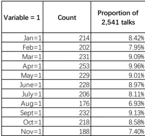
For example, the statistics of 7.~ 12. independent variables representing what day of a
week a given talk is published are shown in Table 2; And statistics of 13.~ 23.
independent variables representing which month of a year a given talk is published are
also shown in Table 3.
Table 2. Different weekdays’ statistics
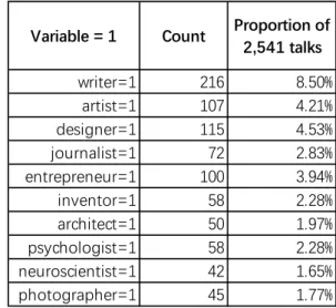
For 24.~ 33. independent variables reflecting a given talk’s themed tag(s) and 34.~ 43.
independent variables reflecting a given talk’s main speaker’s occupations(s), similarly
we use table 4 and table 5 to display their statistics.
Method
In this section, we will focus on how to split our preprocessed data into training,
validation, and test datasets, as well as the machine learning models and methods we
intend to use.
Training, Validation and Test Datasets
Since we are going to use various machine learning models with differing
hyperparameters, we need to split our preprocessed data into training, validation, and test
datasets. Specifically speaking, we will use training and validation datasets to train our
models and select the best one from them based on their different levels of prediction
performances, which can be reflected by mean squared error (MSE). Also, once we have
decided on a certain model, we need the test dataset to report how the selected model can
generally perform on the data outside our model building. Therefore, the test dataset
should not be overlapped with training or validation datasets at any degree.
Also, since we are interested in predicting a TED talk’s popularity, we would like to
build the prediction model in a way of being able to “foresee” the future. Therefore, we
reordered our original dataset by these talks’ published date and picked the most recent
For the 70% talks (1779 observations) left, we will conduct 5-fold cross-validation for
model training and selection.
Machine Learning Models
Corresponding to what has been discussed in the literature review section, we intend to
use two main machine models: linear regression and random forest for our prediction.
Linear Regression
Linear regression assumes linear functional dependency between the independent
variables and the dependent variables. Under this assumption, we will approach our
prediction from the following four methods:
Ordinary least squares (OLS)
OLS is the simplest type of linear regression without regularization or feature selection.
In other words, we will put all 43 independent variables to fit the linear model by the
principle of least squares, which refers to “choosing the regression coefficients so that the
estimated regression line is as close as possible to the observed data, where closeness is
measured by the sum of the squared mistakes made in predicting Y given X.” (Stock and
Watson, 2015).
OLS has its advantages for it is efficient to operate the model building process with
are also evident, for example, without regularization or feature selection, we can include
some useless variables in the model since we have no ideas on how to distinguish which
of these 43 predictors are useful for the model building and this will lead to an overly
complex model or overfitting issues.
After all, OLS could function as the baseline method for others to compare with.
Best feature subset
Best feature subset is a method on top of OLS conducting discrete feature selection. Best
feature subset will allow us to fit separate OLS models for every possible combination of
all independent variables (James et al., 2013). We will use 5-fold cross-validation
approach to determine which of these combinations reaches the best performance with
the smallest training MSE.
Best feature subset can effectively address OLS’s overfitting issues while it usually
involves a much higher level of computation.
Ridge regression
Ridge regression is also invented for controlling model complexity based on OLS.
Instead of directly minimizing OLS’s least squares, ridge regression adds the
regularization/ penalty term 𝜆 ∑& 𝛽𝑗%
'() (where 𝜆 ≥ 0 is a tuning hyperparameter and 𝛽𝑗
the regression coefficients (James et al., 2013). We will use cv.glmnet12’s defaulted
values of 𝜆 and cross-validate them to find the most reasonable hyperparameter.
Although ridge regression helps us control model complexity via 𝜆, it suffers from the
problem of interpretability from the shrunken coefficients. Plus, it will include all 43
variables without doing any feature selection so that it won’t apply well to the cases when
many of the independent variables are useless, which we will never know before running
any models.
LASSO regression
With a similar idea of shrinking coefficients, LASSO regression can be regarded as a
transformation from ridge regression. According to James et al. (2013), the only
difference between these two is LASSO regression adds the term 𝜆 ∑&'()|𝛽𝑗| (where 𝜆 ≥
0 is a tuning hyperparameter, and 𝛽𝑗 refers to any coefficient given p-dimensional model,
which in our case p = 43) instead of 𝜆 ∑& 𝛽𝑗%
'() . We will also use cv.glmnet13’s
defaulted values of 𝜆 and cross-validate them for the optimal hyperparameter.
LASSO regression also controls model complexity via 𝜆 like ridge regression does, while
not like ridge, it does feature selection by yielding zero coefficients for some variables.
Therefore, LASSO regression usually outperforms ridge regression if the case is many of
the independent variables are useless. However, as mentioned, we will never know how
many of our independent variables are useful before running any models. Therefore, it is
Random Forest
The underlying assumption of random forest is the functional dependency between the
independent variables and the dependent variables is non-linear and can be reached by a
collection of decision trees. Random Forest is famous for “decorrelating the trees” by
“not even allowing to consider a majority of the available predictors” at each tree split
(James et al., 2013). For instance, given a total number of independent variables, p, which
is 43 in our case, random forest might only randomly take m = -𝑝 = √43 ≈ 6 of them
for each split in the tree (where m is a hyperparameter deciding how the subset size of
predictors is in each split). Our model building will be based on randomForest14 and
rfcv15’s defaulted number of trees grown and cross-validate the common choices of m,
such as -𝑝, % &, and 5 &, etc.
Random forest is a good complement for linear regression due to it holds a completely
different model building assumption, and it is computationally attractive as well.
Nevertheless, its result cannot be easily interpreted, and the common way to gain insights
from a random forest model is to look at a variable importance plot which only shows the
Result
In this section, we will focus on different models’ prediction performance and the learned
parameter importance from them.
Prediction Performance
For each model, MSE in the raining-validation set will be used to select independent
variables or hyperparameters, and prediction performance will be reflected on each
model’s MSE in the test dataset.
Linear Regression
We will start with illustrating linear regressions’ predication performance.
OLS
Since there is no feature selection or regularization in OLS, we don’t need to do cross
validation in this case. And we can directly apply the OLS model trained from the 70%
training-validation data to the 30% test data for calculating test MSE.
Given the dependent variable is log(daily view), test MSE is 0.7606548; while given
Best feature subset
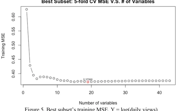
We use 5-fold cross-validation (5-fold CV) for selecting how many variables should be
included in the model to reach the smallest training MSE.
Given the dependent variable is log(daily views), as shown in figure 5, the model
including 19 variables reaches the smallest training MSE (0.37068) and therefore it is
selected. When applied to test data, this model’s corresponding test MSE is 0.8418204.
Figure 5. Best subset’s training MSE, Y = log(daily views)
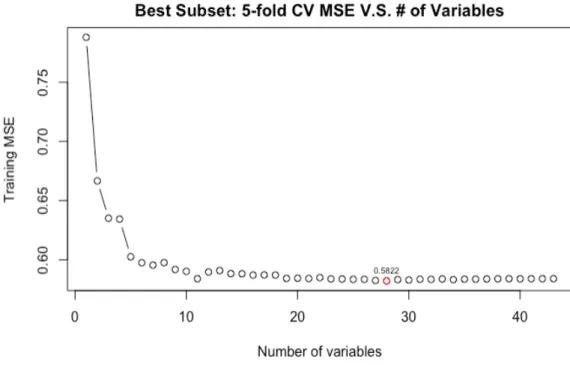
Given the dependent variable is log(daily comments), as shown in figure 6, the model
including 28 features is selected for reaching the smallest training MSE (0.5822), and this
Figure 6. Best subset’s training MSE, Y = log(daily comments)
Ridge
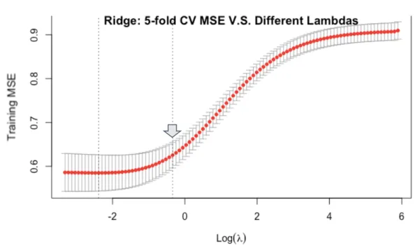
We also use 5-fold CV for selecting which λ should be applied to the model. Inspired by
Hastie and Qian (2014), in instead of using the value of λ that gives minimum
cross-validated training MSE, we choose the largest value of λ within one standard error of the
minimum λ (“lambda.1se”16 , a value saved by cv.glmnet17) to address possible
overfitting issues (as shown in figure 7 and figure 8).
Given the dependent variable is log(daily views), the selected λ (marked in figure 7)’s
Figure 7. Ridge’s training MSE, Y = log(daily views)
Given the dependent variable is log(daily comments), the selected λ (marked in figure
8)’s corresponding model’s test MSE is 0.782524.
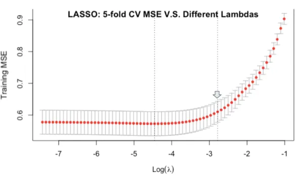
LASSO
We still use 5-fold CV for selecting which λ should be applied to the model. As what we
have done in Ridge, still inspired by Hastie and Qian (2014), in instead of using the value
of λ that yields minimum cross-validated training MSE, we still choose “lambda.1se”18 as
mentioned for generating a more regularized model (as shown in figure 9 and 10).
Given the dependent variable is log(daily views), the selected λ (marked in figure 9)’s
corresponding model only includes 12 features (31 features’ coefficients are assigned as
0), and its corresponding test MSE is 0.8599129.
Figure 9. LASSO’s training MSE, Y = log(daily views)
Given the dependent variable is log(daily comments), the selected λ (marked in figure
10)’s corresponding model only includes 11 features (32 features’ coefficients are
Figure 10. LASSO’s training MSE, Y = log(daily comments)
Random Forest
We also apply 5-fold CV to our selection of which “m” should be optimal for the model
building based on the assumption of random forest.
In the case that the dependent variable is log(daily views), the smallest training MSE is
reached when m = 5, and its corresponding test MSE is 3.19092.
In the case that the dependent variable is log(daily comments), the smallest training MSE
is reached when m = 11, and its corresponding test MSE is 1.13386.
In summary, we create table 6 to display different models’ test MSE. Given the
choices with the smallest test MSE (0.7606548). Meanwhile, given the dependent
variable is log(daily comments), Ridge has the lowest test MSE (0.782524). However, it
is also worth noting that Ridge’s test MSE difference from LASSO’s is fairly small, and
LASSO has a much lower level of model complexity than Ridge, therefore we lean to say
LASSO also performs better the others in the case of log(daily views).
Model OLS Best Subset Ridge LASSO Random Forest
Test MSE given Y = log(daily views)
0.761 0.842 1.094 0.860 3.191
Test MSE given Y = log(daily comments)
0.863 0.881 0.783 0.783 1.134
Table 6. Different models’ test MSE
Since our dependent variables are both log-based, we need to transform them back to the
original unit to better interpret these outperforming test MSEs. With the helpful
instruction from Wang (2020), we have the statements as follows:
Given the dependent variable is log (daily views), test MSE (0.7606548) from OLS
means on average, the prediction deviates from the truth by exp(sqrt(0.7606548))-1 =
139.2061% higher or lower than the original count of daily views.
Given the dependent variable is log (daily comments), test MSE (0.782524) from Ridge
142.2025% higher or lower than the original count of daily comments, while test MSE
(0.7828465) from LASSO means on average, the prediction deviates from the truth by
exp(sqrt(0. 7828465))-1= 142.2466%, which is also not far away from Ridge’s
performance.
Learned Parameter Importance
Not only do we care about different models’ test MSEs indicating different levels of
model performance, but we also would like to explore the learned parameter importance
from them, if possible. In other words, we are eager to learn what variables are
powerful/useless for our prediction to hone our model interpretation.
Linear Regression
In terms of OLS models:
For predicting log(daily views), statistically significant variables (p-value<.05) are
number of language translations (+0.05736), posting gap (-0.00007247), duration in
minutes (+0.03219), mbp (+0.1912), writer (+0.1781), psychologist (+0.3911),
global_issue (-0.3042), culture (+0.09236), design (-0.09074), business (+0.1211), Fri
(+0.2153), Sat (+0.2633), Mar (+0.2108), as well as intercept (3.178). What is in () is
each variable or intercept’s learned coefficient: (+)/ (-) stands for positive/negative effect
Referred to UCLA Statistical Consulting Group19, the intercept, 3.178, is the
unconditional expected mean of log(daily views), and the exponentiated value,
exp(3.178) = 23.99871, is the geometric mean of daily comments. Plus, number of
language translations (+0.05736) means when holding other variables constant, if a TED
talk’s translated languages increase 1 type, the OLS model predicts that its daily views
will increase exp(0.05736)-1= 5.9037%. Also, psychologist (+0.3911) shows that when
holding other variables constant, we expect to see a TED talk delivered by a psychologist
generates exp(0.3911)-1=47.86% more daily views than those which are not. To our
surprise, duration in minutes has an exp(0.03219)-1 = 3.27% positive effect which means
when holding other variables constant, if the talk increases 1 minute, we could expect its
daily views to increase 3.27%. The only explanation we could make is TED talks are so
high-quality that the TED community tends to be immersed watching them, therefore
extending a talk’s duration could trigger more attraction. In other words, in TED
community, a talk is not as engaging or popular if its time duration is too short.
For predicting log(daily comments), statistically significant variables (p-value<.05) are
number of language translations (+0.03944), posting gap (-0.0002041), duration in
minutes (+0.03015), mbp (+0.1295), writer (+0.1629), architect (-0.04516), psychologist
(+0.4010), neuroscientist (+0.3452), culture (+0.1076), TEDx (+0.2035), design
(-0.2558), entertainment (-0.2324), innovation (+0.1961), Sat (+0.5282), Mar (+0.2447), as
well as intercept (-4.662). What is in () is still each variable or intercept’s coefficient: (+)/
(-) stands for positive/negative effect on log(daily comments), and the following number
Still referred to UCLA Statistical Consulting Group20, the intercept, -4.662, is the
unconditional expected mean of log(daily comments), and the exponentiated value,
exp(-4.662) = 0.009447548, is the geometric mean of daily comments. Plus, mbp (+0.1295)
means when holding other variables constant, if U.S. average internet connection speed
increases 1 Mbp, the OLS model predicts that a TED talk’s daily comments will increase
exp(0.1295)-1=13.83%. In addition, Sat (+0.5282) shows that when holding other
variables constant, we expect to see a TED talk published on Saturday generates
exp(0.5282)-1=69.58% more daily comments than those which are not. This makes sense
to us as people are usually more relaxed and more willing to be exposed to Internet-based
contents during the weekend. Mar (+0.2447) means that when holding other variables
constant, we expect to see a TED talk published in March generates
exp(0.2447)-1=27.72% more daily comments than those which are not, and we think this is because
most annual TED conferences hold around March (TED Conference, 2020).
With respect to Best subset models:
Similar variables as OLS’s statistically significant ones are reserved for both dependent
Table 8. Best subset selected variables and their coefficients, Y = log(daily comments)
Given Ridge and LASSO models:
Their introduction of λ makes it hard to interpret independent variables’ effect magnitude
coefficient = 0 to the variables it regards as useless. Therefore, variables with non-zero
coefficients can be deemed as of importance for our prediction.
For predicting log(daily views), LASSO assigned non-zero coefficients to 12 variables,
and they are number of language translations (+), posting gap (-), duration in minutes (+),
mbp (+), writer (+), psychologist (+), global_issue (-), culture (+), design (-), Fri (+), Jan
(-) and March (+), where (+)/ (-) stands for positive/negative effect on log(daily views).
For predicting log(daily comments), LASSO assigned non-zero coefficients to 11
variables, and they are number of language translations (+), posting gap (-), duration in
minutes (+), mbp (+), psychologist (+), culture (+), TEDx (+), design (-), entertainment
(-), Sat (+), and March (+), where (+)/ (-) stands for positive/negative effect on log(daily
comments).
Random Forest
Concerning random forest models:
Even though random forest models do not perform well in the sense of test MSE, and
they are not good at interpretation, these models are still good references to learn
parameter importance because we can generate variable importance plots from them
To sum up, for both dependent variables, the important predictors are very similar, and
the overlapped ones are the number of language translations, mbp, duration in minutes,
and posting gap. Given the main speaker’s occupation, writer and psychologist have the
most noticeably positive effects on a TED talk’s popularity. As for the themed tags,
“culture” stands out for its significant positive influence, while “design” is found to hurt a
talk’s popularity. Besides, Friday, Saturday, and March are good timings for a TED talk
Discussion
This section will discuss our thinking from two aspects: what machine learning prediction
can tell us, and what machine learning prediction cannot tell us.
What Machine Learning Prediction Can Tell us
What machine learning prediction can tell us is how to “detect patterns,” “predict future
data,” and “perform decision making” (Murphy, 2012) based on the prediction model’s
performance and learned parameter importance.
The most evident pattern we have detected is either daily views or daily comments can
function well as the indicator for a TED talk’s popularity, and the important predictors
for them are nearly the same regardless of their different numerical scales. This finding is
also consistent with the previous work (e.g. Ray, Yadav & Garg, 2018) which states a
TED talk’s views and comments are highly related. Therefore, we don’t recommend
predicting a TED talk’s views via comments or vice versa like some work (e.g. Eldor
(2018)’s) did as it would be meaningless like using a feature to predict itself.
Outperforming models can help us “predict future data” (Murphy, 2012). For instance,
once a new TED talk is uploaded online, we could apply the coefficients from OLS to its
all the predictors we use can be known before or as soon as the talk is published. Relying
on the OLS’s test MSE, we would also expect our prediction deviating from the true
values around 140%, which is fairly acceptable given the unit is so small as a talks’ daily
views or comments.
Plus, we can make decisions based on learned parameter importance. For example, the
OLS model predicting log(daily views) tells us that if we increase a talk’s number of
language translations, duration in minutes, or accelerate the U.S. average Internet
connection speed when the talk is published, we could expect more daily views gained.
The OLS model also tells us that if we let a writer/ psychologist be a talk’s main speaker,
or theme the talk on culture/ business instead of design or global issue, or publish it on a
Friday, Saturday or in March, we could also give a plus on the talk’s popularity.
What Machine Learning Prediction Cannot Tell us
What machine learning prediction cannot tell us is strategically speaking, what actions
should TED take in the long term beyond these models and predictors?
Taking the predictor, duration in minutes, as an example, the machine learning prediction
suggests we extend every talk’s duration to gain a higher level of popularity. However,
this won’t make sense in practice. If we only focus on extending a talk’s duration while
ignoring its quality, it might generate more attraction in the short run, however, it will
harm TED’s reputation in the long term. Plus, even if we could maintain each talk’s
as we all know a too-long video could scare people away. The positive effect of duration
in minutes on current TED talks could be a reflection that TED has experience in its
domain, spreading ideas of worth by balancing talks’ duration and attraction. Such
domain knowledge cannot be produced by machine learning prediction while it is of
importance for TED to map out their strategy.
What’s more, machine learning prediction also tells us that if we invite more writers/
psychologists to be TED talks’ main speakers, or theme the talks only on the topics of
culture/ business and avoid topics such as design/ global issue, we could leverage TED
talks’ popularity. Nevertheless, such action goes against the mission TED stands for. We
assume that TED would like to encourage more voices to be heard instead of pursuing a
higher level of popularity by sacrificing its diversity. Therefore, our suggestion is TED
talks’ speakers with different occupations or themed topics could build the
communication bridge among each other and learn the successful experience from
writers/ psychologists or culture/ business topics to improve every talk’s attraction as a
Conclusion
In a nutshell, a TED talk’s popularity can be predicted by its inherent features via
machine learning techniques. We found that the OLS, Ridge, and LASSO models
performed well in the prediction, and we also learned several powerful predictors such as
a talk’s number of language translations, average Internet connection speed, duration,
main speaker’s occupation, as well as its being published timing. With the support of our
experimented models and their corresponding predictors, we detected that a TED talk’s
views or comments are highly related and can either function well as the indicator of
“popularity.” Furthermore, we also looked into how to predict future data and make
sound decisions based on our trained models. In the end, we discussed our suggestion on
how to improve TED talks’ popularity beyond the perspective of machine learning and
emphasized on the importance of domain knowledge in mapping out TED’s long-term
Note
1 https://creativecommons.org/licenses/by-nc-nd/3.0/
2 https://en.wikipedia.org/w/index.php?title=TED_(conference)&oldid=955207602
3 https://www.ted.com/talks
4 https://blog.ted.com/ted-reaches-its-billionth-video-view/
5 https://www.ted.com/talks
6 https://www.ted.com/about/our-organization/how-ted-works
7 https://www.kaggle.com/rounakbanik/ted-talks
8 https://www.kaggle.com/rounakbanik/ted-talks
9 https://www.kaggle.com/rounakbanik/ted-talks
10 https://www.akamai.com/us/en/resources/our-thinking/state-of-the-internet-report/
11 https://www.statista.com/statistics/616210/average-internet-connection-speed-in-the-us/
12 https://www.rdocumentation.org/packages/glmnet/versions/3.0-2/topics/cv.glmnet
13 https://www.rdocumentation.org/packages/glmnet/versions/3.0-2/topics/cv.glmnet
14 https://www.rdocumentation.org/packages/randomForest/versions/4.6-14/topics/randomForest
15 https://www.rdocumentation.org/packages/randomForest/versions/4.6-14/topics/rfcv
16 https://www.rdocumentation.org/packages/glmnet/versions/3.0-2/topics/cv.glmnet
17 https://www.rdocumentation.org/packages/glmnet/versions/3.0-2/topics/cv.glmnet
18 https://www.rdocumentation.org/packages/glmnet/versions/3.0-2/topics/cv.glmnet
19 https://stats.idre.ucla.edu/other/mult-pkg/faq/general/faqhow-do-i-interpret-a-regression-model-when-some-variables-are-log-transformed/
Reference
Akamai Technologies. (May 31, 2017). Average internet connection speed in the United
States from 2007 to 2017 (in Mbps), by quarter [Graph]. In Statista. Retrieved May
01, 2020, from
https://www.statista.com/statistics/616210/average-internet-connection-speed-in-the-us/
Alvarez, T. (2017, October 23). Predicting the Popularity of TED Talks - DZone AI.
Retrieved from https://dzone.com/articles/predicting-ted-talks-popularity
Akamai Technologies. (May 31, 2017). Average internet connection speed in the United
States from 2007 to 2017 (in Mbps), by quarter [Graph]. In Statista. Retrieved May
01, 2020, from
https://www.statista.com/statistics/616210/average-internet-connection-speed-in-the-us/
Banik, R. (2017). TED Data Analysis. Retrieved from
https://www.kaggle.com/rounakbanik/ted-data-analysis
Banik, R. (2017, September 25). TED Talks. Retrieved from
Borges, H., Hora, A., & Valente, M. T. (2016, September). Predicting the popularity of
GitHub repositories. In Proceedings of the 12th International Conference on
Predictive Models and Data Analytics in Software Engineering (p. 9). ACM.
https://dl.acm.org/citation.cfm?id=2972966
Cappallo, S., Mensink, T., & Snoek, C. G. (2015, June). Latent factors of visual
popularity prediction. In Proceedings of the 5th ACM on International Conference
on Multimedia Retrieval (pp. 195-202).
https://dl.acm.org/doi/abs/10.1145/2671188.2749405
Chen, J., Song, X., Nie, L., Wang, X., Zhang, H., & Chua, T. S. (2016, October). Micro
tells macro: Predicting the popularity of micro-videos via a transductive model. In
Proceedings of the 24th ACM international conference on Multimedia (pp.
898-907). ACM. https://dl.acm.org/citation.cfm?id=2964314
Chen, L., & Lee, C. M. (2017). Predicting Audience's Laughter Using Convolutional
Neural Network. arXiv preprint arXiv:1702.02584. https://arxiv.org/abs/1702.02584
cv.glmnet. (n.d.). Retrieved from
https://www.rdocumentation.org/packages/glmnet/versions/3.0-2/topics/cv.glmnet
Deepak Kumar, G. (2017). Lets talk about TED Talks | Kaggle. Retrieved from
Dochev, K. (2019, November 16). Predicting TED Talks Views with ML Models.
Retrieved from
https://www.kaggle.com/dochev/predicting-ted-talks-views-with-ml-models#Predicting-TED-Talks-Views-with-ML-Models
Eldor, T. (2018, January 27). Data Reveals: What Makes a Ted Talk Popular? Retrieved
from
https://towardsdatascience.com/data-reveals-what-makes-a-ted-talk-popular-6bc15540b995
UCLA: Statistical Consulting Group. (n.d.). FAQ How Do I Intepret A Regression Model
When Some Variables are Log Transformed? Retrieved from
https://stats.idre.ucla.edu/other/mult-pkg/faq/general/faqhow-do-i-interpret-a-regression-model-when-some-variables-are-log-transformed/
Fernandes, K., Vinagre, P., & Cortez, P. (2015, September). A proactive intelligent
decision support system for predicting the popularity of online news. In Portuguese
Conference on Artificial Intelligence (pp. 535-546). Springer, Cham.
https://link.springer.com/chapter/10.1007/978-3-319-23485-4_53
Fidelman, M. (2012, June 28). Here's Why TED and TEDx are So Incredibly Appealing
(infographic). Retrieved from
Hastie T. & Qian J. (2014). Glmnet Vignette. Retrieved from
https://web.stanford.edu/~hastie/glmnet/glmnet_alpha.html
Hidayati, S. C., Chen, Y. L., Yang, C. L., & Hua, K. L. (2017, October). Popularity
meter: An influence-and aesthetics-aware social media popularity predictor. In
Proceedings of the 25th ACM international conference on Multimedia (pp.
1918-1923). ACM. https://dl.acm.org/citation.cfm?id=3127903
Hong, L., Dan, O., & Davison, B. D. (2011, March). Predicting popular messages in
twitter. In Proceedings of the 20th international conference companion on World
wide web (pp. 57-58). https://dl.acm.org/doi/abs/10.1145/1963192.1963222
Huang, X., Gao, Y., Fang, Q., Sang, J., & Xu, C. (2017, October). Towards SMP
challenge: Stacking of diverse models for social image popularity prediction. In
Proceedings of the 25th ACM international conference on Multimedia (pp.
1895-1900). ACM. https://dl.acm.org/citation.cfm?id=3127899
How TED works. (n.d.). Retrieved from
https://www.ted.com/about/our-organization/how-ted-works
James, G., Witten, D., Hastie, T., & Tibshirani, R. (2013). An introduction to statistical
Jeon, H., Seo, W., Park, E. L., & Choi, S. (2019). Hybrid Machine Learning Approach to
Popularity Prediction of Newly Released Contents for Online Video Streaming
Service. arXiv preprint arXiv:1901.09613. https://arxiv.org/abs/1901.09613
Liu, Z., Xu, A., Zhang, M., Mahmud, J., & Sinha, V. (2017, May). Fostering User
Engagement: Rhetorical Devices for Applause Generation Learnt from TED Talks.
In Eleventh International AAAI Conference on Web and Social Media.
https://ui.adsabs.harvard.edu/abs/2017arXiv170402362L/abstract
Ma, C., Yan, Z., & Chen, C. W. (2017, November). LARM: A lifetime aware regression
model for predicting youtube video popularity. In Proceedings of the 2017 ACM on
Conference on Information and Knowledge Management (pp. 467-476). ACM.
https://dl.acm.org/citation.cfm?id=3132997
Moser, T. (2017). Predicting a Powerful Idea: A TED Talk Analysis. Retrieved from
https://www.kaggle.com/tristanmoser/predicting-a-powerful-idea-a-ted-talk-analysis
Murphy, K. P. (2012). Machine learning: a probabilistic perspective (pp. 1).MIT press.
O'Sullivan, E., Rassel, G., Maureen, B., & Taliaferro, J. D. (2016). Research methods for
Pappas, N., & Popescu-Belis, A. (2013, June). Combining content with user preferences
for TED lecture recommendation. In 2013 11th International Workshop on
Content-Based Multimedia Indexing (CBMI) (pp. 47-52). IEEE.
https://ieeexplore.ieee.org/abstract/document/6576551
Pappas, N., & Popescu-Belis, A. (2013, July). Sentiment analysis of user comments for
one-class collaborative filtering over ted talks. In Proceedings of the 36th
international ACM SIGIR conference on Research and development in information
retrieval (pp. 773-776). https://dl.acm.org/doi/abs/10.1145/2484028.2484116
Pinto, H., Almeida, J. M., & Gonçalves, M. A. (2013, February). Using early view
patterns to predict the popularity of youtube videos. In Proceedings of the sixth
ACM international conference on Web search and data mining (pp. 365-374). ACM.
https://dl.acm.org/citation.cfm?id=2433443
Provost, F., & Fawcett, T. (2013). Data Science for Business: What you need to know
about data mining and data-analytic thinking. O'Reilly Media, Inc.
randomForest. (n.d.). Retrieved from
Ray, P., Yadav, K., & Garg, G. (2018). TED Talks–A Predictive Analysis Using
Classification Algorithms. Retrieved from
https://www.ideals.illinois.edu/handle/2142/99922
Ray, S., & Business Analytics. (2017, September 9). Commonly used Machine Learning
Algorithms (with Python and R Codes). Retrieved from
https://www.analyticsvidhya.com/blog/2017/09/common-machine-learning-algorithms/
rfcv. (n.d.). Retrieved from
https://www.rdocumentation.org/packages/randomForest/versions/4.6-14/topics/rfcv
Russell, C. J., & Dean, M. A. (2000). To log or not to log: Bootstrap as an alternative to
the parametric estimation of moderation effects in the presence of skewed dependent
variables. Organizational Research Methods, 3(2), 166-185.
https://journals.sagepub.com/doi/abs/10.1177/109442810032002
Stock, J. H., & Watson, M. W. (2015). Introduction to econometrics. (pp.116).
Tanveer, M. I., Hasan, M. K., Gildea, D., & Hoque, M. E. (2019). A Causality-Guided
Prediction of the TED Talk Ratings from the Speech-Transcripts using Neural
Tanveer, M. I., Hassan, M. K., Gildea, D., & Hoque, M. E. (2019). Predicting TED Talk
Ratings from Language and Prosody. arXiv preprint arXiv:1906.03940.
https://arxiv.org/abs/1906.03940
TED Conference. (n.d.). Retrieved from
https://www.ted.com/attend/conferences/ted-conference
TED Staff. (2014, October 30). TED reaches its billionth video view! Retrieved from
https://blog.ted.com/ted-reaches-its-billionth-video-view/
TED Talks. (n.d.). Retrieved from https://www.ted.com/talks
Trzciński, T., & Rokita, P. (2017). Predicting popularity of online videos using support
vector regression. IEEE Transactions on Multimedia, 19(11), 2561-2570.
https://ieeexplore.ieee.org/abstract/document/7903630
Wikipedia contributors. (2020, May). TED (conference). In Wikipedia, The Free
Encyclopedia. Retrieved from
https://en.wikipedia.org/w/index.php?title=TED_(conference)&oldid=955207602
Wingrove, P. (2017). How suitable are TED talks for academic listening?. Journal of
English for Academic Purposes, 30, 79-95.
Wu, Q., Yang, C., Gao, X., He, P., & Chen, G. (2018, November). EPAB: Early Pattern
Aware Bayesian Model for Social Content Popularity Prediction. In 2018 IEEE
International Conference on Data Mining (ICDM) (pp. 1296-1301). IEEE.
https://dl.acm.org/citation.cfm?id=2983859
Yuen, H. (2018). What Makes a Popular TED Talk?. Retrieved from