Spin-correlation coefficients and phase-shift analysis for p+3He elastic scattering

(1)

Spin-Correlation Coefficients and Phase-Shift Analysis for

p+

3

He Elastic Scattering

Timothy Vaughn Daniels

A dissertation submitted to the faculty of the University of North Carolina at Chapel Hill in partial fulfillment of the requirements for the degree of Doctor of Philosophy in the Department of Physics and Astronomy.

Chapel Hill 2009

Approved by:

T. B. Clegg, Advisor

H. J. Karwowski, Reader

W. Tornow, Reader

Y. Wu, Reader

E. J. Ludwig, Reader

(2)

c ○ 2009

(3)

Abstract

TIMOTHY VAUGHN DANIELS: Spin-Correlation Coefficients and Phase-Shift

Analysis for p+3He Elastic Scattering.

(Under the direction of T. B. Clegg.)

A new spin-exchange optical pumping polarized 3_{He target has been used to measure}

(4)

(5)

(6)

(7)

Acknowledgments

This project would not have been successful without the help and support of many people. The value of the patient guidance of my thesis advisor, Professor Thomas Clegg, through all the stages of my graduate studies cannot be overstated. Professor Hugon Karwowski also provided advice and critical feedback throughout. I thank them for their energy, enthusiasm, and accessibility. I am also grateful for Dr. Tatsuya Katabuchi’s intelligence, attention to detail, and cheerfulness.

Many others have contributed to my success at TUNL. Dr. Brian Fisher and Dr. Doug Leonard showed me the ropes when I first arrived. Charles Arnold, Alex Couture, John Cesaratto, and Dr. Astrid Imig were the core team that performed the data-taking, with participation by Dr. Chris Angell. I thank them for hard work on a difficult experiment. I also thank John for tolerating the mess in our office. TUNL staff members John Dunham, Richard O’Quinn, Paul Carter, Bret Carlin, Patrick Mulkey, Brenda West, Dr. Alex Crowell, and Chris Westerfeldt have provided help and advice on subjects including vacuum pumps, beam sources, accelerator operation, radioactive sources, LabVIEW, using the copy machine, and local breweries.

Professor Elizabeth George provided the p+3He phase-shift code along with very helpful advice on the phase-shift analysis. Professor Richard Prior provided the phase-shift code used for p+4_{He scattering. Richard Longland and Dr. Michael Akashi-Ronquest tried valiantly to}

help me make a working GEANT4 target simulation.

Joseph Newton and Dr. Mitzi Boswell have been great friends who pitched in on my experiment, advised me on any number of subjects in physics and life in general, and with whom I enjoyed many beers. My family has also been a source of great support, especially my parents Craig and Sherry. Thanks for believing in me.

Finally, the love and support of my wife Amy have been invaluable.

(8)

(9)

List of Tables

1.1 Global p+3He data set . . . 4

1.2 Theoretical scattering lengths . . . 4

1.3 Experimental scattering lengths . . . 5

3.1 Performance summary of optical pumping cells . . . 21

5.1 Target cell bombarding energies . . . 35

5.2 Estimated precision for TRIM stopping powers . . . 35

5.3 Polarimeter cell bombarding energies . . . 45

5.4 Polarimeter cell analyzing powers . . . 46

5.5 Bombarding energies for target cell calibrations . . . 48

5.6 Bombarding energies forα+3_{He A} y minimum . . . 49

6.1 Points dropped from the phase-shift analysis . . . 63

6.2 Best-fit effective-range parameters . . . 64

6.3 Single-energy phase-shift results . . . 65

6.4 Global phase-shift results . . . 65

7.1 Theoretical scattering lengths . . . 91

7.2 Experimental scattering lengths . . . 91

B.1 Angular momentum coupling . . . 99

B.2 Mixing between orbital angular momentum states . . . 99

C.1 Data at 2.28 MeV . . . 101

C.2 Data at 2.77 MeV . . . 101

C.3 Data at 3.15 MeV . . . 102

C.4 Data at 4.02 MeV . . . 102

(12)

(13)

List of Figures

1.1 Observables for p+3He elastic scattering at 4 MeV . . . 6

2.1 Jacobi vectors for four-nucleon calculations . . . 10

3.1 Overview of the polarized target . . . 14

3.2 A target cell . . . 15

3.3 The sine-theta coil . . . 16

3.4 Sine-theta coil currents . . . 17

3.5 Atomic levels in Rb relevant to optical pumping . . . 18

3.6 An optical pumping cell . . . 18

3.7 Accumulation of3He polarization . . . 19

3.8 Alkali filling station for optical pumping cells . . . 20

3.9 Polarizer schematic . . . 23

3.10 Narrowed laser output . . . 24

5.1 Diagram of chamber setup . . . 34

5.2 Diagram of spin-flip electronics . . . 36

5.3 Chamber detector spectrum for3He(p,p)3He . . . 37

5.4 Chamber detector spectrum for3He(α,α)3He . . . 38

5.5 Polarimeter detector spectrum . . . 38

5.6 Polarimeter background . . . 40

5.7 Chamber background . . . 40

5.8 Wein Filter Calibration . . . 45

5.9 Target cell “spin-down” . . . 47

5.10 Determination of target nmr calibration constant. . . 48

5.11 4He +3He Ay measurements with respect to angle . . . 50

5.12 4He +3He Ay measurements with respect to energy . . . 50

5.13 Instrumental steering effect . . . 52

5.14 Steering of the incoming proton beam and scattered particles by the sine-theta coil magnetic field . . . 52

5.15 Deflection of the incoming beam and scattered particles through anglesα and β, respectively, by the sine-theta coil magnetic field. . . 53

5.16 Angular distribution of Ay0 for p+3He elastic scattering at 2.25 MeV . . . 54

5.17 Calculated instrumental effect for Ay0 at 2.25 MeV . . . 55

5.18 Extrapolation of systematic asymmetries to zero target polarization . . . 55

(14)

6.1 Measurements of Ay0 at 1.60 MeV shown with the phase-shift solution . . . . 63

7.1 Present results at 2.28 MeV . . . 69

7.6 Comparison of 3.15 MeV measurements with theoretical calculations . . . 74

7.9 Results for S-wave phase-shifts . . . 78

7.10 Results for P-wave phase-shifts . . . 79

7.11 Results for D- and F-wave phase-shifts . . . 80

7.12 Results for mixing parameters . . . 81

7.13 Comparison with theoretical S-wave phase-shifts. . . 84

7.14 Comparison with theoretical P-wave phase-shifts . . . 85

7.15 Comparison with theoretical P-wave phase-shifts . . . 86

7.16 Comparison with theoretical D-wave phase-shifts. . . 87

7.17 Comparison with theoretical 3_F 2 and mixing parameters . . . 88

7.18 Triplet P-wave splitting. . . 89

(15)

1

Introduction

According to our modern understanding, protons and neutrons interact through the strong nuclear force to form atomic nuclei. The exact form of the interaction between the “nucleons” has been sought since the proposal of this picture of the nucleus, which in fact predates both the discovery of the neutron and the development of the Standard Model [Bro96]. We now believe that nucleons are composed of quarks and gluons, which interact according to Quantum Chromodynamics (QCD). The force between nucleons should be derivable from this underlying physics in much the same way that molecular forces can be derived from the electromagnetic interaction of atomic electrons. The difficulty of solving QCD in the non-perturbative nuclear regime, however, has prevented that derivation.

A model of the nucleon-nucleon interaction would, in principle, allow one to understand nuclear systems in terms of their constituent nucleons. Such an ab initio approach requires both a workable model of the interaction and computational techniques to solve it for a system of multiple nucleons. Because the interaction has not been derived from QCD, physi-cists have developed various phenomenological models. These models start from the general experimentally-deduced description of the nuclear force, which is described in many nuclear physics textbooks, such as [Ros48, Kap62, Kra88]. The meson exchange model, first proposed by Yukawa in 1935 [Yuk35], accounts for many of the observed features, including finite range, saturation, and spin-dependence. More phenomenological terms are included to describe the short-range repulsion as well as more subtle effects such as charge symmetry breaking. As a result, the models have free parameters which must be adjusted to reproduce experimen-tal data. Several models now exist which accurately describe the extensive NN scattering database [Car98].

(16)

energies find that a three-nucleon force (3NF) must be added to the potential models in order to reproduce the experimental values [Nog02, Nog03]. The models generally reproduce p+d and n+d scattering data well. There are a few significant exceptions to this success, includ-ing the “Ay puzzle”, in which the nucleon and deuteron vector analyzing powers for elastic scattering at low energy are under predicted [Gl¨o96].

In the 4N system, the alpha-particle binding energy is well reproduced without additional interactions beyond the 3NF [Wir00, Nog02, Viv05b], but an even stronger Ay puzzle has been firmly established for p+3He elastic scattering [Fis06]. Despite this and some other discrepancies, observables in many 4N reactions are well reproduced [Del07a, Del07b, Del07c]. For heavier systems, bound-state properties have been calculated up to A=12 [Nav03, Pie04], as well as n+4He elastic scattering phase-shifts [Car07].

The four-nucleon system provides a more difficult challenge to nuclear interaction models than either the 2N or 3N systems, and has been characterized as a “theoretical laboratory” for studying those models [Laz05]. It is more tightly bound than the latter two systems, which should amplify the importance of both the more phenomenological short-range parts of interaction models and 3NF. It is also the lightest nuclear system to exhibit such typical “nuclear” properties as resonances and thresholds [Til92], which makes its accurate description an important milestone for ab initio nuclear physics. Finally, calculating the interaction between four nucleons uses 3NF in higher isospin channels than have so far been available.

The work described in this thesis is aimed at clarifying the comparison of theory and experiment in p+3_{He elastic scattering at the low energies relevant to the A}

y puzzle. A unique set of experimental phase-shifts and mixing parameters for the system would allow a systematic comparison to theoretical models and perhaps establish which partial waves are to blame for the disagreement. Phase-shift analyses, in which these parameters are fit to measured angular distributions of scattering observables, have been attempted since the first measurements were made in 1954, but have historically been hampered by the lack of double-polarized observables.

The global data-set for p+3He elastic scattering below 12 MeV proton energy is sum-marized in Table 1.1. The first measurements were angular distributions of differential cross-section by Famularo in 1954 [Fam54]. A few other cross-section measurements were made in the following several years [Swe55, Lov56, Bro60, Art60] and phase-shift analy-ses [Low54, Fra55] of available data indicated that no spin-dependence was necessary to reproduce those data. In the 1960’s, systematic measurements of precision cross sections became available [Tom62, Cle64, McD64, Tom65, Kav66, Dri66], as well as Ay0 obtained

from double-scattering experiments [Ros60, McD64, Dri66]. Spin-dependent analyses were attempted [Tom62, Cle64, Tom65, Dri67] but wide solution bands were still possible. In the late ’60s, polarized proton beams and polarized 3_{He targets were developed, so that}

(17)

coefficients [McS69, May73], and spin-transfer coefficients [Wei78], as well as cross-sections and Ay0 below 1MeV [Ber80] became available. Phase shift analyses [McS69, Mor69, Bos72,

Bly75, Sza78a, Ber80, Bel85] including these data were better constrained, but the solutions were generally not unique.

The situation improved substantially in 1993, when Alley and Knutson published an energy-dependent, global analysis which included their measurements of Ay0, A0y, and Ayy

at 4, 5.54, 7, 8.5, and 10 MeV, as well as Axx, Axz, Azx, and Azz at 5.54 MeV [All93a]. This dramatic increase in the available spin-correlation data enabled subsequent analyses [All93b, Yos00] to obtain unique solutions. However, a later reanalysis that included the Berg cross-section and analyzing power measurements below 1 MeV, as well as Ay0 measurements

between 1 and 2 MeV, found two distinct solutions [Geo03]. The observables most sensitive to the difference between those solutions are spin-correlation coefficients below 4 MeV. That is not surprising, since no such measurements are present in the database.

The first theoretical calculation for the p+3He elastic scattering observables was by Swan in 1953 [Swa53], who obtained scattering phase-shifts from simple interaction models using variational methods. The first scattering calculation using a realistic model for the system was of the triplet scattering length by Carlsonet al. in 1991 [Car91], who used a variational approach with the AV14+URVII potential. That work was motivated in part by the fact that the triplet scattering length is an important input parameter in calculations of the weak

p-3_{He capture rate, which is the reaction that produces the highest-energy solar neutrinos. The}

singlet and triplet scattering lengths were calculated in 2000 by both Filikhin and Yakovlev [Fil00], who used a cluster reduction method to solve the Fadeev-Yakubovski equations with the Malfet-TjonI-III potential. The scattering lengths were also calculated by the Pisa group, Viviani, Rosati, and Kievski [Viv98], who used the Correlated Hyperspherical Harmonics with the Kohn variational principle to solve the Schrodinger equation with the AV14 and AV18 potentials with a variety of 3N interactions. These three calculations, summarized in Table 1.2, disagree with one another, which implies that experimental values for the scattering lengths might distinguish between them.

Scattering lengths for the system can be obtained from experimental phase shifts by extrapolating a parameterization of the energy dependence of the appropriate phase shift to zero energy, and the three available values are summarized in Table 1.3. Tegner and Bargholtz [Teg83] fit an effective range expansion to the 3S1 phase shifts of [Tom65] and

[Ber80] to obtain the triplet scattering length. The energy dependent phase-shift analyses of [All93b] and [Geo03] determine scattering lengths explicitly as search parameters. The scattering lengths from the two solutions of [Geo03] disagree with each other as well as with those from [All93b], which in turn disagree with [Teg83].

(18)

Table 1.1: Global data set. See section 6.4 for a discussion of [Geo03] data groups.

Reference Ep Observable PSA? in [Geo03]? (group)

[Fam54] 1.01-3.53 σ n y (5)

[Low54] 1.01-3.53 - y

-[Swe55] 4.96, 8.6 σ n n

[Fra55] 1.0-3.5 - y

-[Lov56] 9.75 σ n y (14)

[Bro60] 6.5, 8.3 σ n y (13)

[Art60] 4.96, 8.6 σ n n

[Ros60] 10 Ay0 n n

[Tom62] 2.0-4.8 σ y n

[Cle64] 4.55-11.48 σ y y (11)

[McD64] 4.05-12.79 σ, Ay0 n y (9,10)

[Tom65] 1-11.5 - n

-[Kav66] 0.125-2.0 σ (excitation) n n

[Dri66] 3.38-4.46 Ay0 y excluded

[Mor69] 4.0-10.8 Ay0 y y (12)

[McS69] 8.8 Axz y y (4)

[McS70] 3.86-10.94 A0y y y (4)

[Bos72] 4-10.77 - y

-[May73] 6.80,8.82 Ay0, A0y, Axx, Ayy ? y (3)

[Bly75] 10.5 A0y y y (8)

[Sza78b] 2.3-8.8 A0y y y (7)

[Sza78a] 13.6 - y

-[Wei78] 6.82, 8.82, 10.7 Kxx,Kyy,Kxz n n

[Det79] 1.75-4.5 Ay0 R? y (6)

[Ber80] 0.3-1.0 σ, A0y y y (16,17)

[Bel85] 0-10 - y

-[Geo06] 12.4 A0y n y (15)

[All93a] 4-10 Ay0,A0y,Ayy n y (1,2)

[All93a] 5.54 Axx,Axz,Azx,Azz n y (1)

[All93b] 0-12 - y

-[Yos00] 4-20 - y

-[Viv01] 1.60,2.25 A0y n y (18)

[Geo03] 0-12 - y

-[Fis06] 1-4 σ, A0y y

-Table 1.2: Theoretical scattering lengths Reference as (fm) at (fm)

[Viv98] 11.5 9.13

[Fil00] 8.2 7.7

(19)

Table 1.3: Experimental scattering lengths Reference as (fm) at (fm)

[Teg83] 10.2_±1.4

[All93b] 10.8_±2.6 8.1_±0.5 [Geo03] Soln. 1 15.1_±0.8 7.9_±0.2 [Geo03] Soln. 2 7.2_±0.8 10.4_±0.4

earlier zero-energy calculations. Updated calculations are given in [Fis06]. Pfitzinger and col-laborators [Pfi01] used the Resonating Group Model (RGM) with the AV18, AV8, URIX, and TRA potentials, and compared their results to an updated R-matrix analysis of T=1 data in the four-nucleon system. Most recently, the Lisbon group, Fonseca and Deltuva, has solved the Alt-Grassberger-Sandhas (AGS) equations [Alt67] in momentum space for a variety of modern potentials, including one derived from effective field theory [Del07b]. Quaglioni and Navratil [Qua08] have developed a hybrid method that combines the RGM with the “no core shell model” (NCSM).

These calculations generally compare well with measured angular distributions of cross-section, but underpredict the beam analyzing power by as much as 40%, and the target ana-lyzing power to a lesser extent. Calculations of the Pisa group [Viv05a] are shown with mea-surements from [Fis06] and [All93a] at 4 MeV proton energy in Figure 1.1. Spin-correlation coefficients agree within the large experimental uncertainties. This Ay puzzle is discussed by the various authors in terms of the P-wave phase shifts. In [Fis06], the authors report that Ay is strongly influenced by the combination3P2- 1₂(3P1+3P0), the calculated value of which

is smaller than would be necessary to reproduce the experiment data.

(20)

50 100 150 200 250 300 350

0 20 40 60 80 100 120 140 160 180

d

σ

/d

Ω

(mb/str)

θ_cm (Deg.) [Fis06] av18+urix av18 0 0.1 0.2 0.3 0.4 0.5

0 20 40 60 80 100 120 140 160 180 Ay0

θ_cm (Deg.) [Fis06] av18+urix av18 0 0.02 0.04 0.06 0.08 0.1 0.12 0.14

0 20 40 60 80 100 120 140 160 180 A0y

θcm (Deg.)

[All93a] av18+urix av18 -0.04 -0.02 0 0.02 0.04 0.06 0.08 0.1 0.12 0.14

0 20 40 60 80 100 120 140 160 180 Ayy

θcm (Deg.)

[All93a] av18+urix av18

(21)

2

Theory

2.1 Interaction Models

Two commonly-used models for the force between nucleons are AV18 [Wir95] and CD-Bonn [Mac01]. Both models use one-pion exchange to describe the long-range part of the force, and both include electromagnetic interactions. While the intermediate and short-range physics terms in both models are phenomenological and have about 40 free parameters adjusted to fit experimental data, the two differ in style. The terms in the AV18 potential are written in configuration space and are each of a different functional form with respect to the relevant variables, including position and spin. In this way, each term serves to include a particular feature, such as spin-orbit dependence or charge-independence breaking, into the model. In contrast, the terms of the CD-Bonn potential, written in terms of momentum, each correspond to the exchange of a different meson. A phenomenologicalσ meson is included to account for the two-meson exchange that is important at small distances, and it is primarily the coupling constants and masses of theσ mesons for each partial wave that are fit to data. The former model is therefore more explicitly phenomenological than the latter, but the two are fit to nucleon-nucleon scattering data and measured deuteron properties with similar accuracy.

As discussed in the Introduction, three-nucleon forces are required to reproduce 3_{H and} 3_{He binding energies. The URIX model [Car83], used in [Fis06], is based on two-pion}

ex-change and is written in configuration space. It contains two terms, each of which contains a parameter that is fit to experimental data. The first term describes two-pion exchange through an intermediate delta excitation, and is fit to the3H and 4He binding energies. The second is more phenomenological and is fit to the equilibrium density of nuclear matter.

(22)

parameters of the σ mesons’ coupling to the delta in each partial wave were adjusted to reproduce the Nijmegan NN database. This fit included the readjustment of some of the original nucleon-nucleon parameters. This “CD-Bonn + ∆” potential therefore includes a three-nucleon interaction without actually being fit to any 3N data, and still underbinds3H and 3He, though to a lesser degree than CD-Bonn.

Doleschall and collaborators, in an attempt to exploit the connection between three-nucleon forces and non-local interactions described in [Pol90], have developed so-called “In-side non-local, out“In-side Yukawa” (INOY) potentials. These potentials consist of a purely phenomenological non-local interaction at small distances (within about 3 fm) that smoothly connects to the AV18 potential at larger distances. In its most realistic form [Dol03], the non-locality is restricted to S and D waves and its parameters are fit to the Nijmegan NN database, deuteron properties, and the3He binding energy. The more recent INOY04 [Dol04] and ISuj [Dol08] models include modified P-wave interactions which better describe nucleon-deuteron scattering below 10 MeV, including Ay.

A different approach to constructing nuclear potential models is chiral pertubation theory (χPT). This approach, first used by Weinberg [Wei90], starts with the most general La-grangian consistent with the approximate chiral symmetry of the underlying theory of QCD at low energy. Though interaction models developed in this way contain an infinite number of terms, Weinberg showed that they can be ordered in powers of the ratio of the momentum to the chiral-symmetry breaking scale. Actual potential models, therefore, contain a finite num-ber of terms up to a given order. These terms are associated with either contact interactions or with pion exchange, and the contact terms contain constants which must be fit to NN data. A nucleon-nucleon potential at next-to-next-to-next-to leading order, (N3LO), containing 29 parameters has been constructed by Entem and Macleidt [Ent03]. Terms involving three or more nucleons emerge from the chiral Lagrangian just as NN terms do, so that chiral 3NF’s can be constructed. For example, Navratil [Nav07] discusses the chiral 3NF at N2LO.

2.2 Methods

(23)

overall ground-state energy.

Navratil and Quaglioni [Qua08, Qua09] have developed a hybrid method which combines the ability of the RGM to calculate scattering observables with the accurate use of realistic NN interactions in the No-Core Shell Model (NCSM) to describe the clusters. The interaction between clusters is calculated by considering the interaction of each nucleon in the first cluster with each nucleon of the second through a realistic model. The NCSM uses an average potential derived from the underlying NN interaction in a harmonic oscillator basis. The NCSM results converge to those of an exact calculation provided that enough basis states are used. These calculations are limited both in the cluster excitations and the number of clusters considered, which means that even virtual break-up of the3He is not included. This, in turn, may reduce their accuracy.

In contrast to the RGM, two other methods have been developed which explicitly consider all possible interactions between nucleons without regard to clusters. The Pisa group has used the method of Hyperspherical Harmonics (HH) to calculate 3- and 4-nucleon bound-state and scattering observables [Fis06] with realistic potential models. The wave function is divided into two terms, one of which describes the p+3He system asymptotically while the other describes the system of four nucleons in the interaction region. The former can be written in terms of the S-matrix, which contains the phase-shifts and mixing parameters as described in Chapter 6, through a partial-wave expansion:

ΨLSJπJz

A =

!

L!_S! "

δ_LL!δ_SS!Ω−_LSJJ z−S

J

LS,L!_S!(q) Ω+

L!_S!_JJ z

#

, (2.1)

where Ω−is an incoming spherical wave with relative angular momentum L and total spin S, and Ω+ is an outgoing spherical wave with L! and S!.

The “core” wave function, on the other hand, is expanded in the HH basis. This basis is derived from a set of Jacobi coordinates for the system, a suitable choice for which are, as shown in Figure 2.1:

& x1p =

$

3 2

%

& rm−

&ri+&rj +&rk 3

&

,

& x2p =

$

4 3

%

& rk−

& r_i+&r_j

2

&

, (2.2)

&

x₃_p =&r_j₋&r_i,

where the vectors&r are the locations of the nucleonsi,j,k, andm, and the subscriptprefers to a given permutation of the particles.

(24)

p

k

m

j

i

X

1

X

2p

X

₃

p

Figure 2.1: Jacobi vectors for four-nucleon calculations. Figure adapted from [Fis03].

of a hyperradius:

ρ='x2

1p+x22p+x23p,

(2.3)

hyperangles:

cosφ2p =

x₂_p

'

x2₁_p+x2₂_p

, (2.4)

cosφ3p =

x3p

'

x2₁_p+x2₂_p+x2₃_p ,

as well as the polar angles for each Jacobi vector.

In these coordinates, the kinetic energy operator depends on the hyperradius in one term and on the angular variables, collectively referred to as Ω, in another. The core wavefunction is expanded in the eigenfunctionsYα(Ω) of the angular term, called the hyperspherical harmonic functions:

ΨLSJπJz

C =

!

α

12 !

p=1

uα(ρ)SpαTpαYα(Ωp), (2.5)

(25)

the Kohn variational principle [Koh48] to the complete wavefunction, in which a functional of the Hamiltonian is made stationary with respect to variation of the both the asymptotic scattering-matrix elements and the internal hyperradial coefficients.

The Lisbon group [Del07b, Del08] in contrast, solves the Alt-Grassberger-Sandhas (AGS) [Alt67] equations in momentum space. The method is based on transition operatorsU, such as

U_|φ_"=V _|ψ_", (2.6)

where V is the interaction potential, _|φ_" is an asymptotic free-particle state, and _|ψ_" is the full wave function. Configurations of the four nucleons are considered where: (1) one nucleon is free and the other three bound, and (2) where two pairs are separately bound, and the transitions from the former configuration in the incoming channel to either configuration in the outgoing channel are considered. Each transition has its own operator satisfying the the AGS equations. The scattering observables are extracted from the 4-body transition matrix

T, which is obtained from the four-body transition operator through numerical integration of the momentum-space integrals:

#&p!_|T_|&p_"=_#φ_f_|U_|φ_i_". (2.7)

(26)

(27)

3

Polarized Target

A new spin-exchange optical pumping (SEOP) spin-polarized 3_{He target, described in}

detail in [Kat05], was developed for this work. Previous polarized 3He targets used in low energy charged particle scattering experiments (e.g. protons below 10 MeV) [Roh68, Bak69, Har71, Lee71, Mil89, All93a], have used metastability-exchange optical pumping (MEOP) [Col63], which operates at about 2 mbar3He pressure. With SEOP [Wal97], in contrast, one operates at a3_{He pressure of 1-8 bar. Since thicker targets are advantageous for scattering}

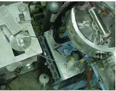
experiments, many polarized3He targets today use SEOP in, for example, high-energy elec-tron [Ant96] and gamma-ray [Kra07] experiments. The low-energy proton beams used in our experiment, however, required that thin foils be used to contain the gaseous3He. This limited gas pressure to 1 bar, and precludes optical pumping of the actual target. This constraint was accommodated in our target, shown in Figure 3.1, by performing the optical pumping in an external polarizer at 8 bar and dispensing 1 bar at a time of polarized 3He into the scattering target.

3.1 Scattering Target

The design of the target cell used to hold polarized 3He during scattering measurement required significant care to minimize the various depolarization mechanisms [Wal97]. In gen-eral, magnetic materials must be avoided, since the presence of inhomogeneous magnetic fields would depolarize the gas. Depolarizing surface interactions, which are not well understood, further limit the choice of materials which come into contact with polarized gas. The target cells used in the experiment, one of which is shown in Figure 3.2, were 5.08 cm diameter Pyrex1 bulbs. Windows were cut along each cell’s mid-plane to allow the low-energy charged particles to emerge. Thin foils were epoxied over the windows to contain the gas. Kapton2 foil and Torr Seal3 _{epoxy were selected based on their emprirically-determined compatibility}

1

Corning Inc. 2

Free samples provided by DuPont, http://www.dupont.com/kapton 3

(28)

Figure 3.1: Overview of the polarized target. The scattering chamber containing the sine-theta coil and target cell is on the right-hand side, with the beam coming in from the top of the picture toward the bottom-right. On the left is the polarizer, where optical pumping was performed, on a cart next to the chamber. The two are connected by a PFA fill-tube.

with3He polarization.

Despite optimization for maintaining 3He polarization, the polarization P of gas in any container will decay over timetaccording to [Dri05]:

P(t) =P₀e−t/T1, (3.1)

whereP0 is the initial polarization and the decay constantT1 is called the “spin-down” time.

The effect of optimizing the cell construction was to lengthen T1 as much as possible, and the spin-down time of the cells used in the experiment was about 2 hours. The T1 for target cells or optical pumping cells, discussed below, could be determined simply by making repeated target polarization measurements as a function of time and fitting Equation 3.1 to the data. A target cell example is shown in Figure 5.9.

(29)

Figure 3.2: Pyrex target cell with Kapton windows. Part of the NMR coil used for mea-suring the target polarization is visible between the cell and its Delrin holder. Figure by T. Katabuchi.

off the cell, which was then placed in a sonic cleaner with a solution of Citronox4 and distilled water.

A uniform magnetic holding field is necessary to define the quantization axis for a sample of polarized 3_{He gas. A Helmholtz coil pair, commonly used to provide uniform magnetic}

fields, failed to provide the necessary uniformity for this project because of steel structures5

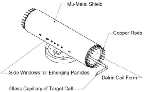
near the scattering chamber. A “sin-theta” coil, shown in Figure 3.3 was therefore developed, which was easily shielded with mu-metal because of its compact design, to provide a field of 0.7 mT with a fractional gradient of 10−3/cm. This device, 30 cm long and 7.5 cm in diameter, contained the target cell and actually fit inside the scattering chamber. It consisted of copper rods pressed onto a hollow cylindrical Delrin form, and each rod carried an electric current proportional to the sine of the angle between that rod and a point on the cylinder as viewed from one of its ends, as illustrated in Figure 3.4. Each current was hardware-regulated to within about 0.1% of its programmed value to maintain uniformity. A mu-metal shield around the outside of the coil prevented non-uniform external fields from reaching the interior. The rod currents were controlled by the polarized target computer through National Instruments LabVIEW FieldPoint modules. This approach allowed the magnetic field direction to be conveniently reversed by stepping through an automated sequence of intermediate field orientations. Similarly, the target spins could be aligned easily along either x or y axes transverse to the beam as necessary for measurements of Ayyand Axx, respectively. The target polarization was measured using pulsed nuclear magnetic resonance (NMR) as described in [Kat05]. A current pulse through a small coil of wire placed against the

4

Alconox, Inc. 30 Glenn St. White Plains NY, 10603 5

(30)

Figure 3.3: The sine-theta coil, shown with a target cell installed. Figure by T. Katabuchi.

cell beam-exit window caused 3_{He spins to precess coherently around the magnetic holding}

field, provided the pulse was at the Larmour frequency determined by the magnitude of the field. The induced voltage from the coherent precession was detected in the coil, and was proportional to both the3_{He polarization and the cell pressure. The pressure-corrected signal,}

therefore, provided a relative polarization measurement which was calibrated by a separate scattering experiment as described in Chapter 5. Similar, though uncalibrated, measurements were made on the optical pumping cells described below.

3.2 Optical Pumping

In optical pumping, circularly polarized light is used to pump atoms placed in an external magnetic field into a particular hyperfine state, as illustrated in Figure 3.5. The wavelength of the light is tuned to the desired atomic transition, but its polarization only allows it to excite transitions to magnetic substates that differ from the ground state by 1 ¯h. The excited atoms decay by collisions with N2 buffer gas to both ground hyperfine states. The fact that

atoms are only pumped out of one ground hyperfine state means that more and more atoms collect in the other, thus creating polarization.

This technique has been exploited to produce nuclear spin-polarization in samples of noble gases since an optically pumped atomic polarization can transfer to nuclear polarization via spin-exchange collisions. MEOP systems optically pump metastable atoms excited by a weak RF discharge, while SEOP optically pump an admixture of alkali metal. In a typical SEOP

3_{He polarizing system, a glass cell is filled with a mixture of}3_{He, N}

(31)

Figure 3.4: Schematic view of the sine-theta coil send end-on. The current in each rod is proportional to the sine of the angle from the intended magnetic field direction. Figure by T. Katabuchi.

the uniform magnetic field of a pair of Helmholtz coils. Circularly polarized laser light at 795 nm illuminates the cell and performs the optical pumping while the cell temperature is kept high enough to ensure sufficient Rb in the vapor phase.

In practice, the accumulation of3_{He polarization p takes hours and saturates below unity}

according to:

p(t) =A(1₋e(−t/τ)), (3.2) wheretis time,A is the saturation polarization, and τ is the “spin-up” time for the system. These limitations result from both the inherently small size of the spin-exchange cross-section and the environmentally dependent loss of accumulated 3He polarization. Depolarization mechanisms include the surface and magnetic gradient interactions discussed above, as well as dipole-dipole interactions between 3_{He nuclei and spin-destruction collisions between Rb}

and 3He [Wal97]. The typical parameters of 8 atm cell pressure and 180 C temperature reflect a balance between increasing the efficiency of optical pumping and minimizing these depolarization mechanisms [Dri05].

3.3 Optical Pumping Cells

The optical pumping cells used in the experiment were spherical bulbs 7.62 cm in diame-ter, as shown in Figure 3.6 and were made of either Ge-180 or Pyrex glass. A pnumatically-actuated anodized aluminum valve, specially ordered from Swagelok6 by Amersham Health, sealed each cell, with a several-inch capillary between the valve and cell to minimize

depolar-6

(32)

5S1/2

m = −1/2 m = +1/2

5P1/2

Figure 3.5: Atomic levels in Rb relevant to optical pumping. Circularly polarized light tuned to the D1 (5S1/2 to 5P1/2) transition excites electrons from only one magnetic substate.

The excited electrons decay to either substate through collisions with N2 buffer gas, but the

population in the “pumped” state is depleted over time, producing polarization.

Figure 3.6: An optical pumping cell. Photo by A. Couture.

ization. The sharp bend in the capillary was made necessary by the tight constraints inside the polarizer solenoid.

The optical pumping cells were loaded with either Rb or a mixture of Rb and K. Though the intended Rb/K ratio was 1:10, the cells used in the experiment actually contained an estimated 1:2 mix [Cou06]. The admixture of K into the “hybrid” or “mixed-metal” cells de-creased the “spin-up” time necessary for the3_{He polarization to saturate by taking advantage}

(33)

0 0.02 0.04 0.06 0.08 0.1 0.12 0.14 0.16 0.18 0.2

0 5 10 15 20 25 30

Polarization

Time (hrs) Rb/K

Rb

Figure 3.7: Accumulation of 3_{He polarization in two optical pumping cells, one of which}

(34)

Figure 3.8: Alex Couture, whose shoulder is visible in the upper left, filling optical pumping cells with alkali metal. The cells are shown with the bakeout oven lowered so that the torch can be used to move (“chase”) the metal down the glass tubes from a retort located out of the picture on the left. The manifold used for evacuation and purging with N2 is visible in

the background toward the right. Photo by A. Couture.

The original pumping cell was prepared by Amersham Health7_{, and was used for}

data-taking until it was accidentally destroyed after Rb blocked its capillary. Replacement cells were loaded [Cou06] with alkali in a system designed to allow the cells, which were attached to a glass manifold, to be baked at 400 C for several days while they were evacuated to 10−8 Torr. A turbo-pump backed by a diaphragm pump was used in order to eliminate the risk of introducing hydrocarbons. The alkali metal ampules were introduced into the manifold before pumping, and during the bakeout were “distilled” by heating with an oxygen-methane torch. After the bake-out was complete, the alkali were “chased” with the torch into the pumping cells, as shown in Figure 3.8

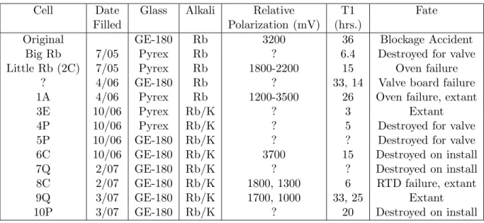
The optical cell performances are summarized in Table 3.1. Several of the cells were unusable because of very short T1 times or because they wouldn’t fit into the oven. None of the replacement cells quite matched the T1 and saturation polarization of the original, and many of their performances degraded over time. Sadly, two of the usable cells were damaged when the oven temperature control failed, while another was destroyed by a malfunction of the computer valve-control. The mixed-metal cells had generally shorter T1 times than the Rb cells.

Interestingly, one cell’s T1 and polarization depended on how it was oriented in the sole-niod. This apparent magnetization could be “degaussed” by connecting the solenoid to AC power through a variac and increasing and decreasing the current. Similar phenomena were reported for Pyrex cells in [Jac01], and were attributed to magnetic domains in the glass.

7

(35)

Table 3.1: Performance and fate of the optical pumping cells used in this work. The amount of information on each cell varies, since those cells with a poor T1 time were never installed on the polarizer, while others would not physically fit into the solenoid. Some cells were accidentally destroyed, while the valves of some poorly performing cells were deliberately removed for use on new pumping cells.

Cell Date Glass Alkali Relative T1 Fate

Filled Polarization (mV) (hrs.)

Original GE-180 Rb 3200 36 Blockage Accident

Big Rb 7/05 Pyrex Rb ? 6.4 Destroyed for valve

Little Rb (2C) 7/05 Pyrex Rb 1800-2200 15 Oven failure

? 4/06 GE-180 Rb ? 33, 14 Valve board failure

1A 4/06 Pyrex Rb 1200-3500 26 Oven failure, extant

3E 10/06 Pyrex Rb/K ? 3 Extant

4P 10/06 Pyrex Rb/K ? 5 Destroyed for valve

5P 10/06 GE-180 Rb/K ? ? Destroyed for valve

6C 10/06 GE-180 Rb/K 3700 15 Destroyed on install

7Q 2/07 GE-180 Rb/K ? ? Destroyed on install

8C 2/07 GE-180 Rb/K 1800, 1300 6 RTD failure, extant

9Q 3/07 GE-180 Rb/K 1700, 1000 33, 25 Extant

10P 3/07 GE-180 Rb/K ? 20 Destroyed on install

3.4 Polarizer

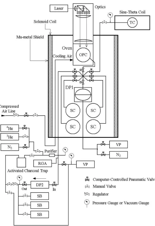
When actually used for data-taking, an optical pumping cell was placed in a gypsum oven, with the capillary and valve emerging from the side to connect to the gas-handling manifold. About 60 W of laser light from an Optopower8 system of diode arrays tuned to the Rb D1 absorption line was fiber-optically coupled to the polarizer. The unpolarized light emerging from the fiber-optic was split into separate linear polarization states, each of which was circularly polarized with quarter-wave plates before passing down into the oven. The oven temperature was computer regulated by blowing laboratory compressed air into it whenever the temperature, measured with an RTD, exceeded a setpoint. The oven was located inside a mu-metal shielded solenoid, 29.4 cm in diameter and about 1m in height, to provide the 0.7 mT magnetic field. This location imposed strict constraints on the dimensions of the pumping cells, and care was required to accomodate the oven, with its electrical and air-cooling connections, as well as the gas-handling apparatus described below, inside the solenoid. A schematic of the polarizer is shown in Figure 3.9.

Gas-handling systems, including pnumatically-actuated valves operated by the target com-puter using LabVIEW, were used to perform a variety of tasks including charging the optical pumping cells with unpolarized 3He, dispensing 1 atm of polaried gas to the target cell,

re-8

(36)

claiming depolarized gas from the target cell, and purifing reclaimed 3_{He in preparation for}

recharging the pumping cell. The pumping cell was filled with 8 bar of unpolarized 3He mixed with about 50 Torr of N2 using a rubber membrane stretched across the middle of

a sphererical plastic cavity. The diaphragm could be “inhaled” or “exhaled” by alternately connecting high-pressure N2 or a mechanical pump to the lower cavity portion. About 2 bar

of gas in the upper cavity portion in the inhaled position would be compressed to 8 bar in the exhaled position. An aluminum manifold connected this “balloon pump” to the pumping cell. Polarized gas was dispensed to the target cell by first equalizing pressure between the pumping cell and that manifold, and then equalizing pressure between the manifold and the target cell, which was connected by a perfluoroalkoxy (PFA)9 fill tube. An external manifold which included a oxygen getter, a liquid-nitrogen trap, and an oil-less diagphram pump was used to remove impurities from gas reclaimed from the target. The entire system had to be leak-tight, since the presence of paramagnetic O2 was poisonous to the3He polarization.

3.5 Narrowed Laser

Some fraction of the broadband laser light used for optical pumping is wasted by being outside the range of wavelengths where absorption by Rb occurs, as shown in Figure 3.10. Thus, concentrating laser power into a smaller bandwidth would put more power into the actual absorption. Motivated by the promising results of [Cha03], a frequency-narrowed laser system was developed as an alternative to the broadband laser for optical pumping [Arn06]. A nominally 50 W Quintessence10 _{diode bar array was placed in an external Littrow cavity}

[Dua95], in which the first-order diffracted light from a diffraction grating is used for feedback. The grating used in this work had 2400 lines/mm. A system of lenses and mirrors, together with the laser and diffraction grating, was mounted on a standard optical table which fit on top of the optical polarizer to direct narrowed light onto the pumping cell. Narrowed light output was typically 0.3 nm FWHM and 30 W. The frequency of the narrowed light was tuned to 795 nm by controlling the temperature of the water-cooled diode array and by adjusting the orientation of the diffraction grating.

The resulting 3He polarization was typically comparable to, though somewhat smaller than, that achieved with the broadband laser. In practice, the optics table, which was mag-netic, had to be removed from the polarizer for dispensing polarized gas to the target, and using the 30 W narrowed laser instead of the 60 W broadband laser required the use of a “hot-watt” resistive heater to keep the oven in the temperature range of 180-220 C necessary for optical pumping. Given the somewhat inferior performance of this system, together with the inconveniences of its use, the broadband laser was used for the majority of data-taking.

9

Obtained from Whitey Co. 318 Bishop Rd. Highland Heights, OH 44143 10

(37)

(38)

0 0.1 0.2 0.3 0.4 0.5 0.6 0.7 0.8 0.9 1

792 793 794 795 796 797 798

Power (mW)

Wavelength (nm)

Narrowed Broadband

(39)

3.6 Performance Summary

The UNC polarized 3He was, in contrast to previous polarized targets for low-energy charged-particle scattering, a high-pressure (1 bar) target whose polarization could be clearly determined. The polarization of the gas dispensed to the target cell varied from 30% using the original optical pumping cell to as low as 10% using various replacement cells, including mixed-metal ones. Unlike systems polarized by continuous optical pumping, the target’s “duty cycle” included time, which was about 24 hours when Rb cells were used and about 12 hours for mixed-metal cells, to polarize new gas. This was generally necessary after 2 or 3 days of data-taking. As described in the remainder of this thesis, the target was used successfully to measure p +3He spin-correlation coefficients between 2 and 6 MeV.

(40)

(41)

4

Observables

This chapter describes the measurement of angular distributions of the beam and target analyzing powers, Ay0 and A0y, and spin-correlation coefficients Ayy and Axx for protons

elastically scattered from3_{He at 5 proton energies between 2 and 6 MeV. These observables}

determine how the scattering at a given energy and angle depends on the spins of the beam and target. The precise definition of the observables and the methods used to measure them are discussed in detail.

4.1 Spin-

1₂

Formalism

4.1.1 One Particle

The spin state of a spin-1₂ particle can be described by a two-component spinor

χ=

*

a b

+

, (4.1)

where a and b represent the probability of the projection along a given axis being measured as “up” or “down”, respectively [Ohl72]. The expectation value for a given observable, rep-resented by operator Ω, is obtained from the spinor,

#Ω_"=χ†Ωχ. (4.2)

We can also use a density matrix to describe the spin state,

ρ=χχ†=

*

|a_|2 ab∗

a∗b _|b_|2

+

. (4.3)

This makes the expectation value of an operator Ω

(42)

The density matrix formalism has the advantage of immediately including the description of anensembleof particles, since a density matrix for the ensemble can easily be constructed,

ρ=

* _,

|a_|2 ,

ab∗

,

a∗b ,

|b_|2

+

. (4.5)

The ensemble average of an operator Ω is likewise given by

#Ω_"=T rρΩ, (4.6)

and the total number of particles is given by

I =T rρ. (4.7)

The polarization of the ensemble with respect to a given axis is given by the ensemble average of that component of the spin

Pi=T rρσi. (4.8)

Polarization varies between -1, when all particles are spin “down”, to +1, when all are spin “up”. A value of 0 indicates equal numbers of up and down.

For later use, the density matrix can be expanded in the basis of the Pauli spin matrices

ρ= 1 2

3 !

j=0

pjσj, (4.9)

wherep0σ0 is defined as the identity matrix.

4.1.2 Two Particles

In the usual spin-coupling scheme, the state of the combined system of two particles can be described in either the basis of the projections of the individual spins or the basis of the total spin and its projection. The density matrix formed from a spinor in the former basis is the same as that obtained from the direct product of the density matrices for the beam and target, and is the one used in the following. Using the expansion 4.9:

ρ= 1 4

3 !

j,k=0

p_jpT_kσ_j_⊗σT_k. (4.10)

The beam and target polarizations are obtained from the expectation values of the operators

(43)

4.2 Observables

The asymptotic wave-function for the elastic scattering of particles with spin is [Got66]:

ψ_∼

%

ei$k·$r+e ikr

r M(E, θ, φ)

&

χ=ψ_inc+ψ_scatt, (4.11)

where

ψ_inc=ei$k·$rχ

is the incoming plane wave describing the incoming beam and

ψscatt =

eikr

r M(E, θ, φ)χ

is the outgoing spherical wave that describes the outgoing particles. Both the overall magni-tude and anisotropy with respect to angles θ and φ of this spherical wave are described by the matrix M.

The fundamental observable for a scattering experiment is the cross-section, which is defined as the ratio of the number of particles scattered into a given element of solid angle to the number of incident particles per area. In terms of particle flux&j:

dσ dΩ =

&jscatt_·_{d &}_A

jinc =

&jscatt_·_r2_d_Ωˆ_r

jinc

Using 4.11 and ignoring interference betweenψinc andψscatt, we obtain:

dσ

dΩ(χi→χf) =|Mf i|

2_, _(4.12)

where _ddσ_Ω(χi→χf) is the cross-section for the transition between particular initial and final statesχi and χf, respectively. The scattering matrix elements, which are functions of energy and angle, therefore contain all the available information about the scattering. For the scat-tering of spin-1/2 particles from spin-1/2 particles, as in p + 3_{He elastic scattering is,}_χ_{is a}

four-component spinor and M is a 4 x 4 matrix.

Equation 4.12 suggests an experiment in which the beam and target are prepared in some polarization state, and then, after the scattering, the final polarization state is fully determined. From an experimental point of view, the latter step requires a second scattering from a known analyzer for both particles, and multiple scattering experiments suffer from low count rates. Fortunately, it is sufficient to determine only the scattered flux when using a polarized beam and target, provided that one can do so for several different inital states. This “spin-correlation” experiment is the type performed for this thesis1.

1

(44)

The differential cross-section for such an experiment is the cross-section for scattering into any final state, and is given by the sum of the cross-sections for transition from each available initial state weighted by the fraction of the ensemble in that initial state:

dσ dΩ =

!

i,f

|Mf i|2ρii,

or, more generally,

dσ

dΩ =T rM ρM

†_, _(4.13)

whereρ is the initial density matrix. Using 4.10, we can see how the scattered yield depends on each combination of each component of beam and target spin,

dσ dΩ =

dσ0

dΩ(θ)

,

pjpTkT rM σj ⊗σkTM†

T rM M† ,

where the T superscript refers to the target. The coefficients that control that dependence are

A_jk(θ) = T rM σj⊗σ T kM†

T rM M† , (4.14)

so that the cross-section can be rewritten

dσ dΩ =

dσ0

dΩ(θ)

!

pjpTkAjk(θ), (4.15)

whereσ0 is the unpolarized cross-section.

This expression must be referred to a specific coordinate system in order to fix the meaning of the observables Ajk. The Madison Convention [Bar71] establishes the coordinate system for polarized scattering experiements. The z axis is along the incoming beam direction, the y axis is in the direction of the incoming beam direction crossed with the direction of scattering, and the x axis is in the direction which makes the system right-handed2. The constraints of time-reversal invariance, parity conservation, and rotational invariance make many of the coefficients identically zero, reducing the expression to

I =I0(1±pyAy0±pTyA0y+pxpTxAxx±pzpTxAzx+pypTyAyy+pzpTzAzz ±pxpTzAxz). (4.16)

The_±refers to scattering to the left or right of the beam, respectively, as necessary to preserve invariance under rotation about the z axis.

scattering elements. In spin-transfer experiments, an unpolarized beam is scattered from an unpolarized target, and the resulting polarization for one of the scattered particles is measured. This type of experiment suffers from requiring two scatterings, as described above.

2

(45)

4.3 Detector Yields

The number of particles detected by a detector at a scattering angleθfrom a beam incident on a gas cell target is proportional to the cross-section,

N =,bpGI. (4.17)

The experimental factors are b, the number of incident beam particles, p, the target pres-sure, the detector efficiency,which describes what fraction of particles entering the detector are actually detected, and the detector “G-factor” [Sil59]. The G-factor describes both the geometrical effects of the detector collimation and the size of the target.

The detector yield as a function of arbitrary spin orientations is therefore

N =,GbpI0(1±pyAy0±pTyA0y+pxpTxAxx±pzpTxAzx+pypTyAyy+pzpTzAzz±pxpTzAxz). (4.18)

For left and right detectors, the yields for different combinations of the beam and target spin orientations as a function of the average polarizations are

L_↑↑=,LGLb↑↑p↑↑I0(1 +pyAy0+pTyA0y+pypTyAyy)

L_↑↓=,LGLb↑↓p↑↓I0(1 +pyAy0−pTyA0y−pypTyAyy)

L_↓↑=,LGLb↓↑p↓↑I0(1−pyAy0+pTyA0y−pypTyAyy)

L_↓↓=,LGLb↓↓p↓↓I0(1−pyAy0−pTyA0y+pypTyAyy)

R_↑↑=,RGRb↑↑p↑↑I0(1−pyAy0−pTyA0y+pypTyAyy)

R_↑↓=,RGRb↑↓p↑↓I0(1−pyAy0+pTyA0y−pypTyAyy)

R_↓↑=,RGRb↓↑p↓↑I0(1 +pyAy0−pTyA0y−pypTyAyy)

R_↓↓=,RGRb↓↓p↓↓I0(1 +pyAy0+pTyA0y+pypTyAyy),

Using these yields, we form the following cross-ratios:

X1 =

-%

L%_↑↑₊_L% _↑↓

L%_↓↑₊_L% _↓↓ & %

R% _↓↑₊_R% _↓↓

R% _↑↑₊_R% _↑↓ &

= 1 +pyAy0 1₋p_yA_y₀

X2 =

-%

L%_↑↑₊_L% _↓↑

L%_↑↓₊_L% _↓↓ & %

R% _↑↓₊_R% _↓↓

R% _↑↑₊_R% _↓↑ &

= 1 +p T yA0y 1₋pT

yA0y

X3 =

-%

L%_↑↑₊_L% _↓↓

L%_↑↓₊_L% _↓↑ & %

R% _↑↑₊_R% _↓↓

R% _↑↓₊_R% _↓↑ &

= 1 +pyp T yAyy 1₋pypTyAyy

(46)

where the primes indicate that we have normalized the yields to the appropriate b and p. The observables are therefore

Ay0=

1

py

%

X1−1

X1+ 1 &

(4.19)

A0y = 1

pT y

%

X2−1

X₂+ 1

&

(4.20)

Ayy= 1

p_ypT y

%

X3−1

X₃+ 1

&

. (4.21)

Similarly, when the beam and target spins are aligned along the x-axis,

A_xx= 1

p_xpT x

X3−1

X₃+ 1. (4.22)

If either the beam or target is unpolarized, only one analyzing power will be non-zero, and the expression 4.19 reduces to the usual cross-ratio expression for analyzing powers,

Ay =

'

L!_↑_R!_↓

L!_↓_R_↑ −1 '

L!_↑_R!_↓

L!_↓_R!_↑ + 1

. (4.23)

(47)

5

Data Collection and Analysis

Spin-correlation coefficients for p+3He scattering were measured according to equations 4.19 through 4.22 using a polarized beam and target. To better understand systematic effects, additional measurements were made of both unpolarized target instrumental asymmetries with either polarized or unpolarized proton beams and the observable A0y with an unpo-larized proton beam. Several other scattering experiments were made in support of these measurements. Briefly, a target cell calibration point was found by the location of an ab-solute minimum in α+3He scattering, frequent target cell calibrations were made using that scattering, the Wein filter spin-precession of the polarized beam was calibrated by maximiz-ing the p+4He asymmetry, and beam polarization was measured with that scattering during data-taking. The performance and analysis of all these measurements are described in detail in this chapter.

5.1 Experimental Set-Up

The measurements were performed using the Triangle Universities Nuclear Laboratory (TUNL) tandem accelerator. Accelerated beams were directed by an analyzing magnet down the 52° beam line to the 62cm scattering chamber, where the Pyrex target cell was installed inside the sin-theta coil as described in the Chapter 3. The chamber set-up is illustrated in Figure 5.1. Beam intensity on the target cell was intially limited to 100nA to avoid damaging the Kapton entrance foils. Experience with failure of the epoxy, especially on the beam exit foils, prompted us to further limit the intensity to 50nA. Even with this reduction, cells lasted no more than a few days.

(48)

Polarimeter Cell Beam

Faraday Cup Target Cell

Sin−Theta Coil Detectors

Figure 5.1: Diagram of Chamber Setup. The polarimeter chamber could be configured with the detectors either horizontal, as shown, or vertical. The polarimeter cell was removed from the beam during data-taking to allow beam to reach the target chamber.

The beam energy was set high enough to offset energy loss, so that the proton energy at the cell’s center was as desired. The bombarding energies for data taken with different thickness entrance foils were slightly different, and the average value, weighted by the error-bars ac-cording to Equation 5.25, was adopted. The uncertainty in the TRIM stopping powers was estimated by comparison with experimental stopping powers [Sri08], as summarized in Table 5.2. A precision of 10% was assigned to cases where no data were present in the relevant energy range.

Polarized beam and target spins were reversed frequently. The beam spin was reversed during data-taking at either 1 or 10 Hz in the sequence +–+-++-, where “+” means “spin-up” and “-” means “spin-down”. The target spin was reversed less frequently, since it required a few seconds to reverse the target’s magnetic field. Polarized target data was collected in the following sequence: the data were collected for about 2.5 minutes with the target spin in one orientation, an NMR measurement was taken, then the spin was flipped, another NMR was taken, and data collection then proceeded with the spin in the second orientation. The target polarization decayed with a 2-3 hour time constant, so this process was stopped when the gas was judged to be too depolarized, generally after about an hour. At that time the gas was exhausted from the target, the target was flushed with research-grade N2, and new

polarized gas, called a “shot”, was dispensed to the target cell.

Scattered particles emerging from the target were detected by four pairs of Si detectors (a mix of surface-barrier and ion-implanted), which could be rotated to the desired angle. The available angles were restricted by the windows in the sin-theta coil’s mu-metal shield to 20°

(49)

Table 5.1: Calculation of target cell bombarding energies for beam which passes first through a Kapton entrance foil and then through the target He gas. The energy at the center of the cell is reported as the bombarding energy. Slightly different bombarding energies which result from the variety of foil thicknesses are averaged together.

Incoming Kapton Entrance Energy After Energy at Average Beam Energy Foil Thickness Entrance Foil Cell Center Energy

(MeV) (µm) (MeV) (MeV) (MeV)

5.77_±0.04 25.4 5.54_±0.04 5.51_±0.04

5.54_±0.03 5.66_±0.04 7.62 5.59_±0.04 5.56_±0.04

4.15_±0.03 7.62 4.06_±0.03 4.02_±0.03 4.02_±0.03 3.54_±0.03 25.4 3.19_±0.03 3.15_±0.03

3.15_±0.02 3.31_±0.03 7.62 3.20_±0.02 3.16_±0.02

3.13_±0.03 17.8 2.86_±0.03 2.81_±0.03

2.77_±0.02 3.13_±0.03 25.4 2.75_±0.03 2.70_±0.03

2.75_±0.02 25.4 2.33_±0.03 2.27_±0.03

2.28_±0.02 2.48_±0.02 7.62 2.34_±0.02 2.29_±0.02

Table 5.2: Estimated precision for TRIM stopping powers Ion Kapton Havar He

proton 7% 5% 3%

α 10% 10% 4%

the target without the 30° snout’s touching the sin-theta coil. The distance from the center of the target cell to the front collimators was about 10.2 cm. Beam current on target was measured by a Faraday cup located about 0.5 m behind the target cell, which was suppressed to -100V. Charge went to ground through a current integrator, which produced the beam current integration (BCI) scaler used as a measure of the relative number of beam particles in each spin state.

Signals from each detector were processed and read into a MicroVAX II1computer running XSYS, as described in [Fis03]. As in that work, spin-routing bits at the ADC interface were used to route data to different data-areas for different spin-states. The use of a polarized target as well as a polarized beam, however, required allocating more data areas, installing an extra scaler module, and modifying the EVL detector sorting codes. Our use of 8 detectors with 6 ADC modules required using two modules for two pairs of detectors, so that the left and right detectors in the first and fourth detector pairs were each routed through a different module, but the left and right detectors for the second and third pairs went through the same module. A logic module was designed and constructed to sort scalers, which in XSYS is done by enabling and disabling the hardware scaler modules as appropriate. A diagram of the

1

(50)

744 Pulser Integrator Current from Faraday cup veto

To bit 1 of ADC interface

to each scaler

to each scaler module

module

module 1 Hz Clock TUNL

Spin State Controller

Fiber + Fiber −

Scaler + Scaler −

TUNL Communications Controller Fan Out 744 Fan Out 744 SF TTL MF2 TTL

Gate & Delay 794

Gate & Delay 794 Fan In 744 Fan Out 744 Fan Out 744 Target transition bit bit Target "down" Target "up" bit

Gate & Delay 794

Gate signal from detector electronics

Gate & Delay 794

60Hz Clock TUNL

Pol. Target Spin Flip Veto

to bit 11 of each ADC interface 433A Dual Sum and Invert 433A Dual Sum and Invert 433A Dual Sum

and Invert Level AdaptorNIM to TTL

Norm Level Adaptor TTL to NIM

688AL Compl. 688AL Discriminator 706 Norm Compl. Level Adaptor NIM to TTL

688AL

TUNL Scaler Control

to bit 12 of each ADC interface To control for each scaler module Clock MF2 SF target beam Fan Out Fan Out Fan Out 744 744

Figure 5.2: Diagram of spin-flip electronics. The scheme is that of [Gei98] with an added signal describing the target spin state.

spin-sorting electronics is given in Figure 5.2.

5.2 Spectra

Spectra obtained from the Si detectors represent histograms of the number of detected particles vs. energy. Typical spectra are shown in Figures 5.3-5.5. The existence of well-defined peaks results from the kinematic determination of the energy of a scattered particle by its mass, its incoming energy, the mass of the target, and the angle of scattering. Knowledge of these factors allows peaks to be identified. The finite width of the peaks is primarily the result of energy straggling in the target. This also causes peak asymmetry, since more energy is lost to straggling by lower-energy particles. The peaks also have a long low-energy tail which arises from scattering on the snout slits.

5.2.1 Peak Sums

(51)

Energy (arbitrary units)

200 400 600 800 1000

Counts

0 2000 4000 6000 8000 10000

He

3

He(p,p)

3

N

14

N(p,p)

14

Pulser

Energy (arbitrary units)

130 135 140 145 150

Counts

0 1000 2000 3000 4000 5000 6000 7000 8000 9000

Summed

State 1

State 2

State 3 State 4

(52)

0 200 400 600 800 1000 0 50 100 150 200 250 300 350 400 Pulser N 14 ) α , α N( 14 α He) 3 , α He( 3 Li 6 ,p) α He( 3 He 3 ) α , α He( 3 State 1 State 2

Figure 5.4: 3He(α,α)3He spectrum at 15.44 MeV and 45°. Individual target spin-states are shown with the summed spectrum

0 200 400 600 800 1000

0 100 200 300 400 Pulser Air(p,p)Air He 4 He(p,p) 4 State 1 State 2 Summed

(53)

peak. Gate sums, scalers, and gate limits were exported from XSYS in text files, which were read into a ROOT script. All further analysis was performed by this script.

Scattering is a random process, so that peak yields are governed by Poisson statistics. The uncertainty in peak area is therefore the square-root of the number of counts. Uncertainties in calculated quantities are determined from uncertainties in peak areas using the standard propagation of error formula [Bev92]. The uncertainty of a function f of n independent quantities ai is

σf =

. / / 0 n ! i=0 % ∂f ∂ai σi &2 + 2 n ! i n ! j>i

σ2_ij∂f ∂ai

∂f ∂aj

(5.1)

where the σ_i2 are the variances in the ai and the σij2 are the covariances between them. The random scattering process insures that there are no correlations between peak yields, so the second term under the radical was often assumed to be zero for this work. When a fitted function was used during analysis, however, correlations between fit parameters were obtained from the error matrix and used in the error propagation.

5.2.2 Background

Two types of background had to be subtracted from the number of counts obtained from summing gates. The first was a flat background, which happened either when a pulser was set below the highest energy peak in the spectrum or when protons scattered from the polarimeter cell itself in addition to the4He gas, as in Figure 5.6. The number of background counts, NA, inside a gate A of width wA set around the peak was estimated from the number of counts NB in a gate B of width wB set to one side of the peak.

NA=NB

wA

w_B (5.2)

σNA = 1

NB

wA

w_B (5.3)

Sometimes two background gates were used, one on either side of the peak. When both gates were used, the sums were averaged.

The second type of background occurred when the 3_{He and} 4_{He peaks overlapped in}

chamber spectra at 30° and 40°. The 4He gas was sometimes added to the cell to measure beam polarization. Two Gaussian peaks modified to mimic energy-loss were fit to these spectra, as in Figure 5.7.

The functional form for a single Gaussian peak with energy loss as a function of channel number x was

y=Ae−12((x+∆x(x)−x0)/σ) 2

Spin-correlation coefficients and phase-shift analysis for p+3He elastic scattering