Choi_unc_0153D_12105.pdf

(1)

Statistical Methods for Joint Analysis of

Survival Time and Longitudinal Data

Jaeun Choi

A dissertation submitted to the faculty of the University of North Carolina at Chapel Hill in partial fulfillment of the requirements for the degree of Doctor of Philosophy in the Department of Biostatistics.

Chapel Hill 2011

Approved by:

(2)

c

○ 2011

Jaeun Choi

(3)

Abstract

JAEUN CHOI: Statistical Methods for Joint Analysis of Survival Time and Longitudinal Data.

(Under the direction of Dr. Jianwen Cai and Dr. Donglin Zeng.)

In biomedical studies, researchers are often interested in the relationship between patients’ characteristics or risk factors and both longitudinal outcomes such as quality of life measured over time and survival time. However, despite the progress in the joint analysis for longitudinal data and survival time, investigation on modeling approach to find which factor or treatment can simultaneously improve the patient’s quality of life and reduce the risk of death has been limited. In this dissertation, we investigate joint modeling of longitudinal outcomes and survival time. We consider the generalized linear mixed models for the longitudinal outcomes to incorporate both continuous and categorical data and the stratified multiplicative proportional hazards model for the survival data. We study both Gaussian process and distribution free approaches for the random effect characterizing the joint process of longitudinal data and survival time.

(4)

(5)

Acknowledgments

I would like to thank my dissertation advisors, Drs. Jianwen Cai and Donglin Zeng, for their expert guidance, deep insights, and thoughtful encouragement throughout my dissertation research process. The lessons I have learned under their direction and the experience I have gained during this process are invaluable. I am grateful to Dr. Jianwen Cai for her financial support as well.

I want to express my sincere gratitude to the committee members, Drs. David Couper, Bahjat Qaqish, and Andrew F. Olshan, for their constructive and perceptive comments. In particular, I am thankful to Dr. Andrew F. Olshan for providing the CHANCE data.

(6)

List of Tables

3.1 Descriptive statistics of predictors in the CHANCE study . . . 43 3.2 Descriptive statistics of outcome variables in the CHANCE study . . . . 44 3.3 Summary of simulation results of maximum likelihood estimation for

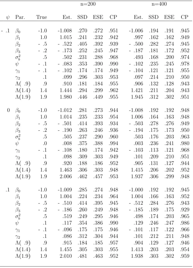
binary longitudinal outcomes and survival time. . . 96 3.4 Summary of simulation results of maximum likelihood estimation for

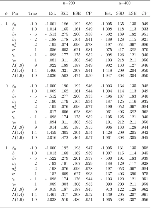
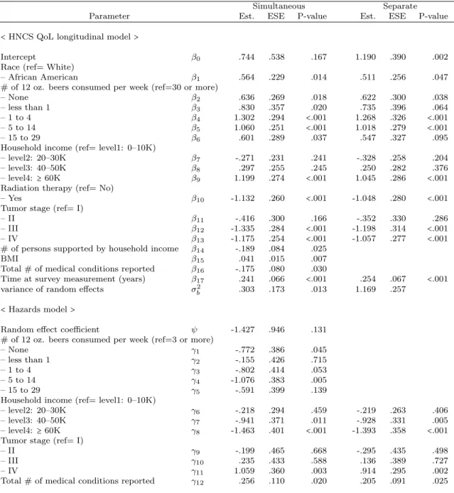
Poisson longitudinal outcomes and survival time. . . 98 3.5 Analyses results for the HNCS QoL and survival time of the CHANCE

study . . . 102

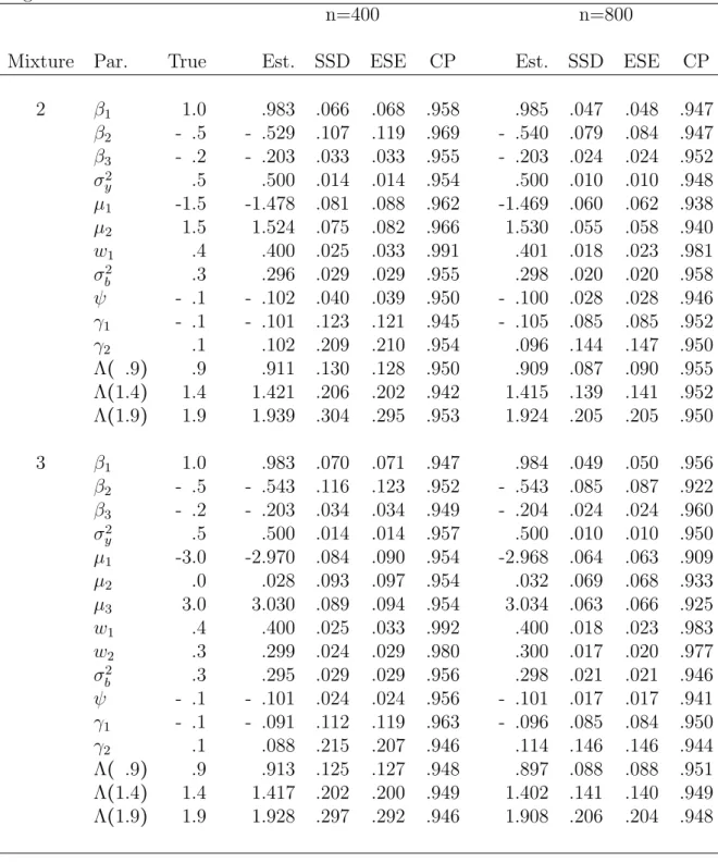
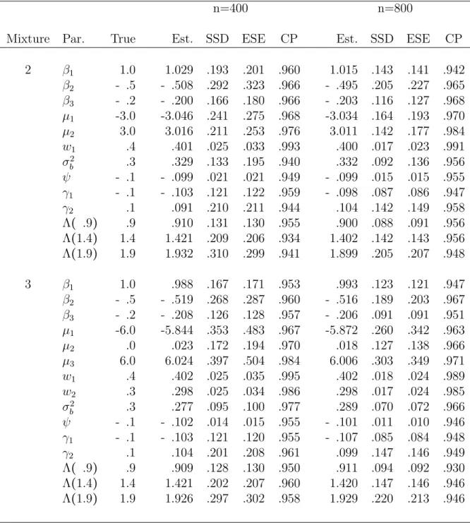
4.1 Summary of simulation results of maximum likelihood estimation using mixtures of Gaussian distributions for random effects in the joint mod-eling of continuous longitudinal outcomes and survival time. . . 168 4.2 Summary of simulation results of maximum likelihood estimation using

mixtures of Gaussian distributions for random effects in the joint mod-eling of binary longitudinal outcomes and survival time. . . 170 4.3 Summary of simulation results of sensitivity for model-misspecification . 172 4.4 Summary of simulation results: Frequencies on the selected number of

Normal distributions in mixture (n=200) . . . 175 4.5 Results from final models of simultaneous and separate analyses for the

Quality of Life and survival time for the CHANCE study . . . 178

(11)

5.2 Summary of simulation results from maximum likelihood estimation (MLE) and maximum penalized likelihood estimation (MPLE) in the si-multaneous modeling of binary longitudinal outcomes and survival time (n=400). . . 203 5.3 Analyses results from maximum likelihood estimation (MLE) and

(12)

List of Figures

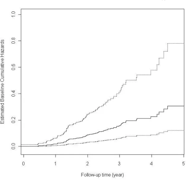
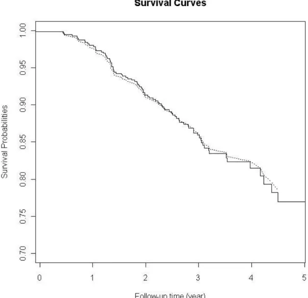
3.1 Estimated baseline cumulative hazards (solid line) with 95% confidence interval (dashed lines) by the simultaneous analysis of HNCS QoL lon-gitudinal outcome and survival time . . . 103 3.2 Kaplan-Meier estimates (solid line) and the predicted survival

proba-bilities based on the simultaneous analysis of HNCS QoL longitudinal outcome and survival time (dashed line) . . . 104

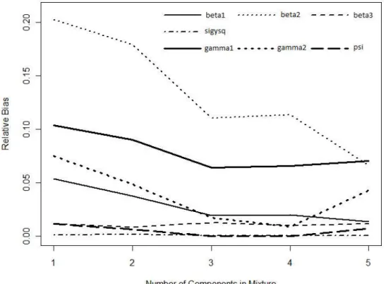
4.1 Density plots of random effects from simulation results of sensitivity for model-misspecification . . . 173 4.2 Relative bias plot of parameters in longitudinal and hazard models (thin

and thick lines respectively) from simulation results of sensitivity for model-misspecification . . . 174 4.3 Estimated baseline cumulative hazards (solid line) with 95% confidence

interval (dotted lines) by the simultaneous analysis of HNCS QoL longi-tudinal outcome and survival time . . . 181 4.4 The predicted conditional longitudinal trend based on the simultaneous

models (solid line) and the empirical longitudinal trend (dotted line) based on the empirical longitudinal HNCS QoL satisfaction probabilities (dots) . . . 182

5.1 Plot of ratios of mean squared errors (MSEs) of maximum penalized likelihood estimator (MPLE) to maximum likelihood estimator (MLE) for parameters of predictors in longitudinal and hazard models (n=200, 400) . . . 207 5.2 Plot of ratios of user times of maximum penalized likelihood estimator

(13)

Chapter 1

INTRODUCTION

(14)

1.1 Joint Analysis for Survival Time and Longitudinal

Cate-gorical Measurements of Quality of Life in Head and Neck

Cancer Patients

(15)

1.2 Joint Modeling of Survival Time and Longitudinal

Out-comes with Flexible Random Effects

(16)

1.3 Penalized Likelihood Approach for Joint Analysis of

Sur-vival Time and Longitudinal Outcomes

(17)

Chapter 2

LITERATURE REVIEW

In this section, we review the statistical literature for : 1) failure time models, 2) longitudinal data models and methods, 3) joint models of failure time and longitudinal data, and 4) penalized quasi-likelihood approach. The organization of the rest of this section is as following. We review literature on statistical methods for Cox proportional hazard models of univariate failure time and frailty models of correlated failure times in section 2.1, and, for generalized linear models with random effects and parameter estimation of longitudinal data in section 2.2. In section 2.3, we review the literature on statistical methods for joint models of failure time and longitudinal data. Lastly, we review penalized quasi-likelihood approach for generalized linear mixed model and bias correction for the estimator in section 2.4.

2.1 Failure Time Models

(18)

why this problem cannot be handled via straightforward regression approaches: First, the dependent variable of interest (failure/survival time) is most likely not normally distributed, which is a serious violation of an assumption for ordinary least squares multiple regression. Survival times usually follow a skewed distribution. Second, there is the problem of censoring, that is, some observations will be incomplete.

We summarize the Cox proportional hazard model for the univariate failure time, which is not based on any assumptions concerning the nature or shape of the underlying survival distribution, in section 2.1.1, and the frailty model for the correlated failure time, which formulates the nature of dependence explicitly, as an extension of the Cox model in section 2.1.2.

2.1.1 Univariate failure time model

The Cox proportional hazards model (Cox, 1972) has been the most widely used pro-cedure to study the effects of covariates on a failure time. The Cox model assumes that the hazard function for the failure timeT associated with a covariate vectorZ is given by

λ(t∣Z) =λ0(t)exp{βT0Z(t)}, t≥0 (2.1)

whereλ0(t)is an unspecified baseline hazard function andβ0is ap×1 vector of unknown

regression parameters. The model (2.1) is semi-parametric in that the effect of the covariates on the hazard is explicitly specified while the form of the baseline hazard function is unspecified. The model (2.1) assumes that hazard ratios are proportional across groups or subpopulations over time, and the regression coefficientβ₀ represents the log hazard ratio for one unit increase in the corresponding covariate given that the other covariates in the model are held at the same value.

Let C denote the potential censoring time and X=min(T, C) denote the observed

(19)

process and ∆ = I(T ≤ C) be an indicator for failure, where I(.) is an indicator function. The failure time is assumed to be subject to independent right censorship. Let(Ti, Ci,Zi)(i=1, . . . , n)be n independent replicates of (T, C,Z) and τ denote the

study end time.

The regression parameterβ₀ in (2.1) can be estimated by applying standard asymp-totic likelihood procedure to the ‘partial’ likelihood function, introduced by Cox (1975),

L(β) = n

∏

i=1

[ exp{βTZi(Ti)}

∑n

l=1Yl(Ti)exp{β

T

Zl(Ti)}

]

∆i

,

where Zi(Ti) is the covariate vector for the subject failing at Ti, and Zl(Ti) is the

corresponding covariate vector for thel-th member who is at risk at Ti. The estimator

for β₀, denoted by ˆβ, is obtained by the partial likelihood score function

U(β) =

n

∑

i=1

∆i{Zi(Xi) −

S(1)(

β, Xi)

S(0)(_β_{, X}

i)

},

where S(0)(_β_{, t}) =_n−1∑n

i=1Yi(t)exp{β ′

Zi(t)}, S(1)(β, t) =n−1∑ni=1Yi(t)exp{β

′

Zi(t)}

Zi(t). The maximum partial likelihood estimator ˆβ, defined as the solution to the

unbiased score equationU(β) =0, has been shown to be approximately normal in large samples with meanβ₀ and with a covariance matrix that can be consistently estimated by−{∂U(β)

∂β ∣β=βˆ} −1

(Andersen & Gill, 1982; Tsiatis, 1981). Iterative procedures, such as Newton-Raphson method and EM algorithm, are commonly used to solve the score equation.

(20)

from Cox model, Clayton & Cuzick (1985) and Hougaard (2000) proposed frailty model for clustered failure data in which subjects may or may not experience the same type of event but they may be correlated because subjects are from the same cluster. In the frailty model, Cox proportional hazards model is used to model each individual’s hazard function, and then an unobserved cluster-specific frailty is introduced into each model to account for within-cluster correlation. This frailty model is reviewed in the next section 2.1.2.

2.1.2 Correlated failure time model

The Cox model (2.1) in the previous section 2.1.1 assumes the independent failure times. In many biomedical studies, however, the independence between failure times might be violated, which may arise because study subjects may be grouped in a manner that leads to dependencies within groups, or because individuals may experience multiple events. For such data, there are two main approaches: the marginal model approach which leaves the nature of dependence among related failure times completely unspecified and the frailty model approach which formulate the nature of dependence explicitly. When the interest resides in estimating the effect of risk factors and the correlation among the failure times are considered as a nuisance, the marginal model approach suits this purpose very well. However, in some settings, one might be interested in the strength and nature of dependencies among the failure time components, for which the frailty models have been proposed and studied by many authors. We focus on frailty model in this section.

(21)

consider a Cox proportional hazards model for subjectiwith respect to thekth event :

λik(t∣wi) =wiλ0(t)exp{βT0zik(t)} (2.2)

where the frailty terms {wi}, i = 1, . . . , n are assumed to be independent and to arise

from a common parametric density. The commonly used one is the gamma distribution, mostly for mathematical convenience. Various choices are possible for this density, which include the positive stable distributions, the inverse Gaussian distributions and the log-normal distributions. Note that β₀ in (2.2) generally needs to be interpreted conditionally on the unobserved frailty. The frailty model approach is particularly sensible, when the strength of the dependence of failure times is of interest.

The parameter estimates are obtained through the EM algorithm, making use of the partial likelihood expression in the maximization step as shown in Klein (1992). An alternative approach is to use a penalized partial likelihood for the estimation of the shared frailty (Therneau & Grambsch, 2001).

Troxel & Esserman (2004) proposed a novel application of frailty models to assess the correlation between survival and quality of life in oncology. A frailty parameter is a random effect that allows the variability among clusters of measurements to be incor-porated into survival models. The collected quality of life outcomes are dichotomized in order to apply the multivariate survival methods. In spite of the necessity of the conversion, the discretization of the quality of life scores from a continuous to a failure-time structure leads to the loss of information available from continuous quality of life data.

(22)

frailty, with subjects nested within clusters) are used in the model with the responses linked at the higher cluster level. This additional level of random effects makes the model more flexible. They used a mixed effects model for the repeated measures that incorporates both subject- and cluster-level random effects, with subjects nested within clusters. A Cox frailty model is used for the survival model as it allows for between-cluster heterogeneity. Then they link the two responses via the common between-cluster-level random effects, or frailties, using a multivariate normal assumption for computation ease (Li & Lin, 2000). More joint models of survival and longitudinal data are reviewed using different models in section 2.3.

2.2 Longitudinal Data Models and Methods

The defining feature of a longitudinal study is that individuals are measured repeatedly through time. Longitudinal data require special statistical methods because the set of observations on one subject tends to be intercorrelated. This correlation must be taken into account to draw valid scientific inferences.

(23)

2.2.1 Generalized linear model with random effects

The linear random effects model is applied where the response is assumed to be a linear function of explanatory variables with regression coefficients that vary from one individual to the next. This variability reflects natural heterogeneity due to unmeasured factors, which can be represented by a probability distribution. Correlation among observations for one person arises from their sharing unobservable variables, Ui.

The random effects GLM has the following general specifications:

1. Given the random effectsUi, the responsesYi1, . . . , Yini are mutually independent and follows a distribution from the exponential family with density

f(yij∣Ui;β) =exp[{(yijθij−ψ(θij))}/φ+c(yij, φ)]. (2.3)

The conditional moments, µij = E(Yij∣Ui) = ψ′(θij) and vij =Var(Yij∣Ui) = ψ′′(θij)φ,

satisfy h(µij) = xTβ+dTijUi and vij = v(µij)φ where h and v are known link and

variance functions, respectively, and xij and dij are covariate vectors of length p and

q, respectively. dij is a subset of xij.

2. The random effects, Ui, i =1, . . . , m, are mutually independent and identically

distributed with density function f(Ui;G).

Another fundamental assumption of the random effects model is that the Ui are

independent of the explanatory variables. A model of this type is sometimes referred to as a “latent variable” model (Bartholomew, 1987).

2.2.2 Maximum likelihood and conditional likelihood methods

LetU = (U1, ..., Um). In maximum likelihood approach, U is treated as a set of

(24)

variance matrix G. In conditional likelihood approach, the random effects is treated as if they were fixed parameters to be removed from the problem, so that we need not rely on the second assumption in the previous section 2.2.1.

Maximum likelihood approach treats Ui as a sample of independent unobservable

variables from a random effects distribution. Then, the likelihood function for the unknown parameter δ, which is defined to include bothβ and the elements of G, is

L(δ;y) = m

∏

i=1

∫

ni ∏

j=1

f(yij∣Ui;β)f(Ui;G)dUi, (2.4)

which is the marginal distribution of Y obtained by integrating the joint distribution ofY and U with respect toU. In some special case such as the Gaussian linear model, the integral in (2.4) has a closed form, but for most non-Gaussian models, numerical methods are required for its evaluation.

To find the maximum likelihood estimate, we solve the score equations obtained by setting to zero the derivative with respect to δ of the log likelihood. Considering the ‘complete’ data for an individual to comprise (y_i,Ui) and restricting attention to

canonical link functions (McCullagh & Nelder, 1989) for which θij = h(µij) = xTijβ+ dT_ijUi, then the ‘complete data’ score function for β has a particularly simple form

Sβ(δ∣y,U) =

m

∑

i=1

ni ∑

j=1

xij{yij−µij(Ui)} =0, (2.5)

where µij(Ui) = E(yij∣Ui) = h−1(xT_ijβ+dTijUi). The observed data score functions Sβ(δ∣y)are defined as the expectations of the complete data score functionsSβ(δ∣y,U)

in (2.5) with respect to the conditional distribution ofU giveny. This gives,

Sβ(δ∣y) =

m

∑

i=1

ni ∑

j=1

(25)

The score equations forG can similarly be obtained as

SG(δ∣y) =

1 2G

−1{

m

∑

i=1

E(UiUTi ∣yi)}G

−1−m

2G

−1=

0. (2.7)

A common strategy to solve for the maximum likelihood estimate of δ is to use the EM algorithm (Dempster et al., 1977). This algorithm iterates between an E-step, which involves evaluating the expectations in the above score equations (2.6) and (2.7) using the current values of the parameters, and an M-step, in which we solve the score equations to give updated parameter estimates. The dimension of the integration involved in the conditional expectation isq, the dimension ofUi. Whenqis one or two,

numerical integration techniques can be implemented reasonably easily. (e.g. Crouch & Spiegelman, 1990) For higher dimensional problems, Monte Carlo integration methods can be used. (e.g. the application of Gibbs sampling in Zeger & Karim, 1991)

Gaussian distribution is a convenient model used most for the random effects. When the regression coefficients are of primary interest, the specific form of the random effects distribution is less important. However, when the random effects are themselves the fo-cus, inferences are more dependent on the assumptions about their distribution. Lange & Ryan (1989) suggested a graphical way to test the Gaussian assumption when the response variables are continuous. When the response variables are discrete, the same task becomes more difficult. Davidian & Gallant (1992) developed a non-parametric approach to estimate the random effects distribution with non-linear models.

In conditional likelihood approach for the generalized linear models with random effects (Diggle et al., 1994; McCullagh & Nelder, 1989), the main idea is to treat the random effects Ui as a set of nuisance parameters to be removed, and to estimate β

(26)

Treating U as fixed, the likelihood function for β and U is

L(β,U;y) = m

∏

i=1

ni ∏

j=1

f(yij∣β,Ui) ∝ m

∏

i=1

ni ∏

j=1

exp{θijyij−ψ(θij)}, (2.8)

where θij = θij(β,U). Restrict attention to canonical link functions (McCullagh &

Nelder, 1989) for which θij =xTijβ+d T

ijUi, the likelihood in (2.8) can be written as

L(β,U;y) =exp{βT ∑ i,j

xijyij + ∑

i

UT_i ∑

j

dijyij− ∑

i,j

ψ(θij)}.

Hence, the sufficient statistics for β and Ui are ∑i,jxijyij and ∑i,jdijyij respectively,

and ∑_i,jdijyij is sufficient for Ui for fixed β.

The conditional likelihood is proportional to the conditional distribution of the data given the sufficient statistics for the Ui, and the contribution from subject i has the

form

f(y_i∣ ∑ j

dijyij =bi;β) =

f(y_i;β,Ui)

f(∑_jdijyij =bi;β,Ui)

= f(∑jxijyij =ai,∑jdijyij =bi;β,Ui)

f(∑_jdijyij =bi;β,Ui)

. (2.9)

For a discrete generalized linear model, this expression (2.9) can be written as

P(y_i∣ ∑ j

dijyij =bi;β) = ∑

Ri1exp(β

T

ai+UTi bi)

∑Ri2exp(β

T _∑

jxijyij +UTi bi)

,

whereRi1 is the set of possible values foryi such that∑jxijyij =ai and ∑jdijyij =bi,

and Ri2 is the set of values for yi such that ∑jdijyij =bi. The conditional likelihood

for β given the data for all m individuals simplifies to

L(β∣y,∑

j

dijyij =bi) =

m

∏

i=1

∑Ri1exp(β

T

ai)

∑R exp(β T

∑ni

j 1xijyij)

(27)

For simple cases such as the random intercept model, the conditional likelihood is reasonably easy to maximize (Breslow and Day, 1980). By the analogy with the usual score equations derived from the full likelihood, the score equations obtained from the conditional likelihood (2.10) can be used to get maximum conditional likelihood estimator for β.

The random effects generalized linear models in biostatistics have been studied enormously including the following literatures providing useful additional references: Laird & Ware (1982); Stiratelliet al.(1984); Gilmour et al.(1985); Schall (1990); Zeger & Karim (1991); Waclawiw & Liang (1993); Solomon & Cox (1992); Breslow & Clayton (1993); Drum & McCullagh (1993); Breslow & Lin (1995) and Lin & Breslow (1996).

2.3 Joint Models of Failure Time and Longitudinal Data

Joint analysis of survival time and repeated measurements has been intensively studied in recent literature. The most models which have been used in such analysis can be categorized into a selection model or a pattern mixture model. The selection model would answer the question regarding how one’s quality of life affects death and the pattern-mixtrure model would describe the pattern of quality of life given one’s death time. However, research interest is also often in finding which factor or treatment can simultaneously improve the patients’ quality of life and reduce the risk of death, which can be studied by the simultaneous analysis of quality of life and survival.

Let Y denote the longitudinal outcomes, for example, quality of life, then Y are realizations of a latent process ˜Y measured with errors. Let T denote survival time.

(28)

effects; then it is fed into the model ofT given ˜Y as a linear predictor. Selection model is reviewed in section 2.3.1.

In the pattern mixture model, a model is assumed for longitudinal outcome Y

conditional on survival timeT (Wu and Carroll, 1988; Wu and Bailey, 1989; Hogan and Laird, 1997) and interest focuses on estimating parameters in the model for longitudinal outcome.

Simultaneous modeling serves the purpose to model both the process for quality of life, Y, and survival time, T, given observed covariates X. Zeng & Cai (2005) proposed such a model of quality of life Y following normal distribution and survival time T by the observed covariates X and by unobserved factors with normal density. This approach is reviewed in section 2.3.2. It is noted that this approach is different from either selection model or pattern-mixture model, although mathematically, all three models can be regarded as different ways of writing the distribution of (T, Y) given covariates.

2.3.1 Failure time model with longitudinal covariates

(29)

1975) the closest observed covariate value prior to that time, often termed ‘last value carried forward’. It is well known (Prentice, 1982) that substituting mis-measured val-ues for true covaiates in the Cox model leads to biased estimation. Another strategy for estimation of the proportional hazard regression parameters is a two-stage approach (Pawitan & Self, 1993; Tsiatis et al., 1995) : First, the mixed effects model is fitted to data at each risk set assuming normality for both random effects and intra-subject error from which empirical Bayes estimates of the individual random effects are ob-tained as described by Laird and Ware (1982). Then, predictors for the covariate for each subject at each failure time based on the relevant fit are substituted for the true covariate values in the Cox partial likelihood. This approximate method uses regression calibration (Carroll et al., 1995) to reduce bias of the naive approach but still yields biased estimators for large measurement error. Alternatively, the joint likelihood of the survival and longtidinal data may form the basis for inference. DeGruttola & Tu (1994) assumed the covariate process and survival times to be multivariate normal and fitted the model via parametric maximum likelihood. Wulfsohn & Tsiatis (1997) adopted the less rigid proportional hazards relationship and used nonparametric maximum likeli-hood, but continued to assumed normal random effects. Henderson et al.(2000) used normal random effects in Gaussian covariate stochastic processes. Faucett & Thomas (1996) assumed normality and took a Bayesian approach.

(30)

In this section, we focus on the conditional score estimation approach by Tsiatis & Davidian (2001) since the fundamental idea of the maximum likelihood approach, which has been mostly studied with distributional assumption of random effects by many authors, is same as that reviewed in section 2.3.2.

For each subject i (i=1, ..., n), let Ti and Ci denote time to failure and censoring,

respectively, where time on studyVi =min(Ti, Ci) and failure indicator ∆i=I(Ti ≤Ci)

are observed; all variables are independent across i. Let Zi denote time-independent

covariates andXi(u)denote time-dependent covariates at time ufor subject i; for

sim-plicity, assume Xi(u) is scalar, but generalization to vector-valued Xi(u) is

straight-forward. Assume that Xi(u) follows a subject-specific linear model Xi(u) =α0i+α1iu,

where αi = (α0i, α1i)T are the intercept and slope for i. The covariate process Xi(u)

is not directly observed; rather, longitudinal measurements Wi(tij) are obtained at

ordered times ti = (ti1, ..., timi)

T_{, for} _t

imi ≤ Vi, where Wi(tij) = Xi(tij) +eij, with

ei = (ei1, ..., eimi)

T_{. The errors} _e

ij reflect uncertainty in measuring Xi(u) at tij and

are assumed identically normally distributed and independent with mean zero and variance σ2_{, independent of} (_T

i, Ci, αi, Zi, ti, mi). More precisely,

(ei∣Ti, Ci, αi, Zi, ti, mi)∼Nmi(0, σ

2_I

mi),

whereImithe mi-dimensional identity matrix.

The survival model assumes that the hazard of failure is related to Xi(u) and Zi

through a proportional hazards regression model; that is,

λi(u) = lim du→0

du−1_pr{_u≤_T

i<u+du∣Ti ≥u, αi, Zi, Ci, ei(u), ti(u)}

= lim

du→0

du−1

pr{u≤Ti<u+du∣Ti ≥u, αi, Zi}

(31)

where λ0(u) denotes an unspecified baseline hazard function, the collection of times

of longitudinal measurements up to and including u is denoted by ti(u) = (tij ≤ u),

ei(u) = (eij ∶tij ≤u), and η is (q×1). The model (2.11) shows explicitly the nature of

the assumption that timing of measurements and censoring are noninformative. Interest focuses on estimation of the parameters γ and η.

Let ˆXi(u)be the ordinary least squares estimator ofXi(u)using all the longitudinal

data up to and including time u, that is based on ti(u). This requires at least two

longitudinal measurements on iup to and including u, for ti2≤u. Define the counting

process increment

dNi(u) =I(u≤Vi<u+du,∆i=1, ti2≤u)

and the ’at risk’ process Yi(u) = I(Vi ≥ u, ti2 ≤ u); that is, dNi(u) puts point mass

at time u corresponding to the observed death time for the i-th subject as long as this occurs after the second longitudinal measurement, andYi(u) is the indicator that

subject i is at risk with at least two longitudinal measurement at time u. Then the estimator ˆXi(u), conditional on {αi, ti(u), Yi(u) =1, Zi}, is normally distributed with

meanXi(u) =α0i+α1iuand varianceσ2θi(u), the usual variance of the estimated mean

ˆ

Xi(u)atuusing data up to and includingu, which depends on timing of measurements

for i up to and including u. For Xi(u) =α0i+α1iu, θi(u) = 1/mi,u+ (u−t¯i,u)2/SSi,u,

whereti(u)contains mi,u time-points tij with mean ¯ti,u, SSi,u= ∑ mi,u

j=1 (tij−t¯i,u)

2_.

At any time u, given that i is at risk at time u so that Yi(u) = 1, random effects

αi, longitudinal measurements taken up to and including time u at times ti(u), and

time-independent covariatesZi, the conditional density for {dNi(u) =r,Xˆi(u) =x}is

(32)

which equals

[λ0(u)duexp{γXi(u)+ηTZi}]r[1−λ0(u)duexp{γXi(u)+ηTZi}]1−r

{2πσ2_θ

i(u)}

1 2

exp[−{x−Xi(u)}

2

2σ2_θ

i(u)

];

thus, the conditional likelihood of {dNi(u),Xˆi(u)} given {Yi(u) = 1, αi, Zi, ti(u)}, up

to order du, is

[λ0(u)duexp{γXi(u) +ηTZi}]dNi(u)

exp[−{Xˆi(u) −Xi(u)}2/{2σ2θi(u)}]

{2πσ2_θ

i(u)}

1 2

=exp[Xi(u){γdNi(u) +

ˆ

Xi(u)

σ2_θ

i(u)

}]{λ0(u)exp(ηTZi)du}dNi(u)

{2πσ2_θ

i(u)}

1 2

exp{− ˆ

X2

i(u) +Xi2(u)

2σ2_θ

i(u)

}.

This representation implies that, conditional onYi(u) =1,

Si(u, γ, σ2) =γσ2θi(u)dNi(u) +Xˆi(u)

is a complete sufficient statistic forαi, suggesting that, at each time u, conditioning on

Si(u, γ, σ2)would remove the dependence of the conditional distribution on the random

effects αi. Then, the conditional intensity process defined as

lim

du→0

du−1

pr{dNi(u) =1∣Si(u, γ, σ2), Zi, ti(u), Yi(u)}

is equal to λ0(u)exp{γSi(u, γ, σ2) −γ2σ2θi(u)/2+ηTZi}Yi(u). Reasoning underlying

the conditional score estimator follows by analogy with that for estimators for the proportional hazards model with no measurement error.

The conditional intensity ofdN(u) =Σn

j=1dNj(u), given{Si(u, γ, σ

2)_{, Z}

i, ti(u), Yi(u),

i=1, ..., n},is λ0(u)E0(u, γ, η, σ2), where E0(u, γ, η, σ2) = ∑nj=1E0j(u, γ, η, σ

2)_,

(33)

This suggests that a reasonable estimator for dΛ0(u)=λ0(u)du is given by

dΛˆ0(u) =dN(u)/E0(u, γ, η, σ2).

By analogy with the usual score equations derived from the partial likelihood in a proportional hazard model, (γ, η) can be obtained by solving the (q+1) ×1 set of estimating equations

n

∑

i=1

∫ {Si(u, γ, σ2), ZiT}T{dNi(u) −E0i(u, γ, η, σ2)dΛˆ0(u)} =0,

which upon substitution ofdΛˆ0(u) for dΛ0(u), may be written as

n

∑

i=1

∫ {Si(u, γ, σ2), ZiT}T{dNi(u) −

dN(u)E0i(u, γ, η, σ2)

E0(u, γ, η, σ2)

} =0 (2.12)

Defining E1j(u,γ, η, σ2)={Sj(u,γ, σ2),ZjT}Texp{γSj(u,γ, σ2)−γ2σ2θj(u)/2+ηTZj}Yj(u),

E1(u, γ, η, σ2) =

n

∑

j=1

E1j(u, γ, η, σ2),

and interchanging the sums in (2.12), the estimating equations are expressed as

n

∑

i=1

∫ [{Si(u, γ, σ2), ZiT}

T ₋E1(u, γ, η, σ2)

E0(u, γ, η, σ2)

]dNi(u) =0. (2.13)

With no measurement error, σ2 = _{0, (2.13) is identical to the score equations for the}

maximum partial likelihood estimator of Cox (1975). With Xi(u) time-independent

andσ2 _{known, the equations are asymptotically equivalent to those proposed by}

Naka-mura (1992). There is an alternative semiparametric estimator with time-independent covariates studied by Buzas (1998).

(34)

Allen-Mersh (2000) proposed the application of a random effect selection model in the form of a trivariate Normal model for the joint analysis of QoL response and log survival time. The trivariate Normal model presented by Schluchter is a model that has been discussed in the context of drop-out. This model is a random effect selection model that assumes that the random parameters of a subject’s underlying response profile such as intercept and slope of QoL response over time, and the logarithm of the survival time follow a trivariate Normal distribution.

Xu & Zeger (2001) developed latent variable models for joint analysis of longitu-dinal data comprising repeated measures and times to events, starting with the latent variable formulation of Fawcett and Thomas(1996), and extending and adapting it to the problem of identifying whether a longitudinal variable Y is a useful auxiliary or surrogate variable for event timeT given other covariates. The linking linear predictor of Y and T was assumed to follow a Gaussian stochastic process suggested by Diggle (1988).

Song, Davidian, & Tsiatis (2002) assumed that the random effects have distribu-tion in a plausible class with smooth densities, in mixed effects model for longitudinal covariates process belonging to proportional hazards model of event time. They used a class of smooth densities studied by Gallant & Nychka (1987). One speculation of Song et al.(2002) is that it is possible that the likelihood based approach using normality

yields consistent estimator even when normality is a mis-specification under certain ‘nice’ conditions through their simulations.

(35)

Tsi-atis & Davidian 1998). Their theoretical results further confirmed that nonparametric maximum likelihood estimation, which was proposed in the literature (Wu & Carroll, 1988; Tsiatis, DeGruttola and Wulfsohn, 1995; Wulfsohn & Tsiatis, 1997), provided efficient estimation. Additionally, it was also shown that the profile likelihood function can be used to give a consistent estimator for the asymptotic variance of the regression coefficients.

Tseng, Hsieh, & Wang (2005) proposed the joint modeling of longitudinal covariates and survival time using accelerated failure time since the accelerated failure time model is an attractive alternative to the Cox model when the proportionality assumption is not appropriate to describe the relationship between the survival time and longitu-dinal covariates. Hsieh, Tseng, & Wang (2006) recently studied maximum likelihood approach for the joint modelling of survival time and longitudinal covariates in details more.

Song & Wang (2007) proposed semiparametric approaches for joint modeling of longitudinal covariates and survival data with time-varying coefficients. To deal with covariate measurement error, they proposed a local corrected score estimator and a local conditional score estimator which are semiparametric methods in the sense that there is no distributional assumption needed for the underlying true covariates. Li, Wang, & Wang (2007) proposed score functions, named generalized sufficient and conditional scores, for the joint models of a primary endpoint and multiple longitudinal covariate processes by adjusting the bias resulted from the approaches by Li, Zhang & Davidian (2004).

2.3.2 Simultaneous model of failure time and longitudinal data

(36)

(2001b) and Zeng & Cai (2005) proposed similar simultaneous models of continuous longitudinal outcome Y and survival time T. However, while in the model by Xu & Zeger a common latent process is shared by bothY andT, Zeng & Cai allow individual random effects to affect quality of life and survival time very differently.

In the approach by Zeng & Cai (2005), quality of life and survival time are modeled through parametric and semiparametric models, respectively, assuming a linear mixed effect model for the longitudinal outcomes of quality of life and a multiplicative haz-ard model for survival time. In both models, observed covariates, which are included as predictors, are assumed to be either time-independent or external time-dependent variables. Unobserved factors enter the models as subject-specific random effects so as to account for unobserved heterogeneity.

For subject i given T > t and the observed history till time t, the longitudinal outcome of quality of life Yi(t) at timet follows the linear mixed effect model,

Yi(t) =Xi(t)β+X˜i(t)ai+i(t),

whereXi(t)and ˜Xi(t)are the row vectors of the observed covariates and can be

com-pletely different or share some components,i(t)is a white noise process with mean zero

and varianceσ2

y, andai denotes a vector of subject-specific random effect of dimension

k0 following a multivariate normal distribution with mean zero and covariance matrix

Σa, and β is a column vector of coefficients for Xi(t). The random effect ai reflects

the unobserved heterogeneity and is allowed to differ for different levels of covariates ˜

Xi(t).

For the survival timeTi given the observed covariates, the observed history till time

(37)

multiplicative hazards model,

λ(t)exp{W˜ i(t)(φ○ai) +Wi(t)γ},

whereWi(t)and ˜Wi(t) are the row vectors of the observed covariates and may share

the same components, φ is a vector of parameters, and λ(t) is the baseline hazard rate function, and γ is a column vector of coefficients for Wi(t). For the dependence

parameterφbetween quality of life and survival time,φ=0 means the dependence can be fully attributed to the observed covariates, and φ≠0 implies that such dependence may also be due to some latent variables.

Supposing the survival time is possibly right censored with completely random right-censored time Ci, and assuming Ni, the number of the observed quality of life

measurements for subject i, to be non-informative about parameters of interest, the observed data fromn subjects are

(Ni, Y_ij,Xj_i,X˜ j

i), j =1, . . . , Ni, i=1, . . . , n,

(Zi,∆i,{(Wi(t),W˜ i(t)) ∶t≤Zi}), i=1, . . . , n,

where for subjecti,(Y_ij,X_ij,X˜_ij)is thej-th observation of(Yi,Xi,X˜i),Zi=min(Ti,Ci),

and ∆i =I(Ti ≤Ci). Interests are estimating and making inference on the parameters θ= (σy,Σa,β,φ,γ)and the baseline cumulative hazard function Λ(t) = ∫

t

0 λ(s)ds.

(38)

function for(θ,Λ) is expressed as

L =

n

∏

i=1

∫_a[(2πσ2

y)

−Ni/2_exp{−(_Y

i−Xiβ−X˜ia)T(Yi−Xiβ−X˜ia)/2σy2}

λ(Zi)∆iexp{∆i(W˜i(Zi)(φ○a) +Wi(Zi)γ)−∫ Zi

0

eW˜ i(s)(φ○a)+Wi(s)γ

dΛ(s)}

(2π)−k0/2∣

Σa∣−1/2exp{−aTΣ

−1

a a/2}]da,

where Yi denotes the vector of (Y_i1, ..., Y_iNi)T, Xi denotes the matrix of ((X1i)T, ...,

(XNi

i )T)T, ˜Xi denotes((X˜

1

i)T, ...,(X˜ Ni

i )T)T, and k0 is the dimension of a.

EM algorithms are employed for the maximum likelihood estimates for (θ,Λ) over a set in which θ is in a bounded set and Λ belongs to a space consisting of all the increasing functions with Λ(0) = 0. It is clear that the maximum likelihood estimate for Λ can be chosen as a step function with jumps only at the observed failure times. In the EM algorithm, ai is considered as the missing statistics for i=1, . . . , n. Therefore,

the M-step solves the conditional score equation from the complete data given the observations, where the conditional expectation can be evaluated in the E-step. The iteration between E-step and M-step is conducted until the estimates converge. The final maximum likelihood estimate for (θ,Λ) is denoted by(θˆ,Λˆ).

The variance estimator for ˆθ is obtained by using the profile likelihood function whose logarithm is defined aspln(θ) =maxΛn−1∑ni=1qi(θ,Λ)whereqi(θ,Λ),i=1, . . . , n,

(39)

2.4 Penalized Quasi-Likelihood Approach

In the view of the cumbersome and often intractable numerical integrations required for a full likelihood analysis, several suggestions were made for approximate inference in generalized linear mixed models and other nonlinear variance component models. One approach was proposed by Breslow & Clayton (1993) with some modifications to a Laplace expansion in order to motivate standard estimating equations that may be solved by iterative application of normal theory variance components procedures. In this section, we mainly review the penalized quasi-likelihood for generalized linear mixed model proposed by Breslow & Clayton (1993), and the bias correction in the penalized quasi-likelihood estimators proposed by Breslow & Lin (1995).

2.4.1 Penalized quasi-likelihood in generalized linear mixed

model

(40)

com-ponents and (in absolute value) fixed effects when applied to clustered binary data, but the situation improves rapidly for binomial observations having denominators greater than one.

Within the framework of the generalized linear mixed model(GLMM), given an unobserved vector of random effects, observations are assumed to be conditionally in-dependent with means that depend on the linear predictor through a specified link func-tion and condifunc-tional variances that are specified by a variance funcfunc-tion, known prior weights and a scale factor. The random effects are assumed to be normally distributed with mean zero and dispersion matrix depending on unknown variance components.

Consider hierarchical model and denote yi, i = 1, . . . , n, as the i-th observation

of a univariate response variable with two vectors xi and zi of explanatory variables

associated with the fixed and random effects respectively. The n responses may be blocked in some way, for example when they involve repeated measures on the same subject. Suppose that, given a q-dimensional vector b of random effects, the yi are

conditionally independent with means E(yi∣b) =µbi and variances Var(yi∣b) =φaiv(µbi),

where v(⋅) is a specified variance function, ai is a known constant (e.g., the reciprocal

of a binomial denominator) and φ is a dispersion parameter that may or may not be known. The conditional mean is related to the linear predictorηb

i =xTi α+zTi b by the

link function g(µb

i) = ηib, with inverse h = g−1, where α is a p vector of fixed effects.

Denoting the observation vector byy= (y1, . . . , yn)T and the design matrices with rows

xT

i and zTi byX and Z, the conditional mean satisfies

E(y∣b) =h(Xα+Zb).

(41)

of yi, the dispersion parameter φ is fixed at unity. In other cases, however, it may

be estimated together withθ as a parameter in the covariance matrix of the marginal distribution ofy.

The integrated quasi-likelihood function used to estimate (α,θ) is defined by

eql(α,θ)∝ ∣_D∣−1/2

∫ exp[ − 1 2φ

n

∑

i=1

di(yi;µbi) −

1 2b

T_D−1

b]db, (2.14)

wheredi(y, µ) = −2∫ µ y

y−µ

aiv(u)du denotes the deviance measure of fit. If, conditionally on

b, the observations are drawn from a linear exponential family with variance function

v(⋅), then the deviance is well known to equal to the scaled difference 2φ{l(y;y, φ) − l(y;µ, φ)}, where l(y;µ, φ) denotes the conditional likelihood of y given its mean µ

(McCullagh & Nelder 1989). In this case ql(α,θ) represents the true log-likelihood of the data. The primary difficulty in implementing full likelihood inference lies in the integrations needed to evaluate ql and its partial derivatives.

The equation (2.14) can be written as c∣D∣−1/2

∫ e−κ(b)_d_b_{, and then applied with}

Laplace’s method for integral approximation (Barndorff-Nielsen & Cox 1989; Tierney & Kadane 1986). Letκ′ _and_κ′′ _{denote the} _q _{vector and}_q×_q _{dimensional matrix of}

first-and second-order partial derivatives ofκwith respect tob. Ignoring the multiplicative constant c, the approximation yields

ql(α,θ) ≈ −1

2log∣D∣ − 1 2log∣κ

′′(˜_b)∣ −_κ(_b˜)_, _(2.15)

where ˜b=˜b(α,θ) denotes the solution to

κ′= −

n

∑

i=1

(yi−µb_i)zi

φaiv(µb_i)g′(µb_i)

+D−1

(42)

that minimizes κ(b). Differentiating again with respect to b, we have

κ′′ = −

n

∑

i=1

zizTi

φaiv(µbi)[g′(µbi)]2

+D−1+

R

≈ ZTW Z+D−1

, (2.16)

where W is the n×n diagonal matrix with diagonal terms wi = {φaiv(µb_i)[g′(µb_i)]2}−1

that are recognizable as the GLM iterated weights (Firth 1991, McCullagh & Nelder 1989). The remainder termR= − ∑n_i=1(yi−µ

b i)zi

∂ ∂b[

1

φaiv(µb_i)g′₍_µb

i)]

has expectation 0 and is thus, in probability as a function of n, of lower order than the two leading terms in the equation ofκ′′_. _R_equals₀_{for the canonical link functions, for which}_g′(_µ) =_v−1(_µ)

(McCullagh & Nelder 1989). Combining (2.14)–(2.16) and ignoringR leads to

ql(α,θ) ≈ −1

2log∣I+Z

T_{W ZD}_{∣ −} 1

2φ

n

∑

i=1

di(yi, µ

˜_b

i) −

1 2 ˜

bTD−1˜

b, (2.17)

where ˜b is chosen to maximize the sum of the last two terms.

Assuming that the GLM iterative weights vary slowly (or not at all) as a function of the mean, the first term in this expression is ignored, andαis chosen to maximize the second. Thus (αˆ,ˆb) = (αˆ(θ),ˆb(θ)), where ˆb(θ) =˜b(αˆ(θ)), jointly maximize Green’s (1987) PQL

− 1 2φ

n

∑

i=1

di(yi, µbi) −

1 2b

T

D−1

b. (2.18)

Differentiation with respect to α and b leads to the score equations for the mean parameters:

n

∑

i=1

(yi−µbi)xi

φaiv(µbi)g′(µbi)

= 0

n

∑

i=1

(yi−µbi)zi

φaiv(µbi)g′(µbi)

= D−1

(43)

For the estimation of variance component θ, we substitute the maximized value of (2.18) into (2.17) and evaluate W at (αˆ(θ),ˆb(θ)), which generate an approximate profile quasi-likelihood function ql(αˆ(θ),θ) for inference on θ. To make degrees-of-freedom adjustments that account for the fact that ˆα rather than α appears in the approximate profile quasi-likelihood function ql(αˆ(θ),θ), we modify ql(αˆ(θ),θ) to the REML version (Patterson & Thompson 1971) in practice. By differentiating the modified profile quasi-likelihood with respect to the components of θ, we obtain the estimating equations for the variance parameters.

2.4.2 Bias correction in penalized quasi-likelihood

The approach proposed by Breslow & Clayton (1993) have been applied to a wide variety of generalized linear mixed models. Although the approximate procedure have been demonstrated to work reasonably well for discrete data problems with moderate to large cell frequencies, their performance is less satisfactory when the data are sparse. Breslow & Lin (1995) derived the general expressions for the asymptotic biases in approximate estimators of regression coefficients and variance component, for small values of the variance component, in generalized linear mixed models with canonical link function and a single source of extraneous variation. Their numerical studies of a series of matched pairs of binary outcomes showed that the first order estimators of the variance component are seriously biased, and they provided the easily computed correction factors which produce satisfactory estimators of small variance components. Their variance correction factors for a series of matched pairs of binomial observations rapidly approach one as the binomial denominators increase.

Let the data be in a series of m clusters of observations(yij, xij), where iidentifies

the cluster, j = 1, . . . , ni identifies subjects within clusters and xij are p-vectors of

(44)

random effectbi, the observations in thei-th cluster are assumed to have log conditional

density

li(α;bi) = ni ∑

j=1

aij

φ {yijηij−h(ηij)} +c(yij;φ), (2.19)

where ηij = xTijα+bi denotes a linear predictor, the aij are prior weights, and φ is

a known scale parameter. This restriction to canonical link functions (McCullagh & Nelder, 1989) implies that the the conditional means µbi

ij = E(yij∣bi) = g−1(ηij) and

variances Var(yij∣bi) =φa−_ij1v(µ_ijbi) are related via g′=1/h′′ =1/v for link and variance

functions g and v, respectively. The bi are assumed to be a random sample from a

normal population with mean 0 and variance θ. Thus the likelihood for the observed data is

L(α, θ) =

m

∏

i=1

Li(α, θ) = m

∏

i=1

(2πθ)−1

2∫ eli(α,b)−b 2

/2θ

db. (2.20)

Denote (α,ˆ θˆ) as the true maximum likelihood estimator. For approximations, we con-sider the derivatives l(k)

i =∂kli/∂bk. Using Laplace method (e.g. Barndorff-Nielson &

Cox 1989), the likelihood function in (2.20) may be approximated by expanding the integrand in a Taylor series about its maximizing value ˜bi, where ˜bi = ˜bi(α, θ) solves

˜_b_i ₌_θl(1)

i (α,˜bi). Setting ˜l

(k)

i =l

(k)

i (α,˜bi), a quartic expansion gives

Li(α, θ) ≏ (2πθ)−

1

2 exp(˜l_i−

˜_b2

i

2θ) ∫ exp{

1 2(

˜

l(2)

i −

1

θ)(b−

˜_b

i)2}

×{1+1 6 ˜

l(3)

i (b−˜bi)3+

1 24

˜

l(4)

i (b−˜bi)4}db

= (1−θ˜l(2)

i )

−1

2 exp(˜l_i−

˜_b2

i

2θ){1+

θ2˜_l(4)

i

8(1−θ˜l(2)

i )2

}

≏ (1−θ˜l(2)

i )

−1

2 exp{˜l_i−

˜

b2

i

2θ +

θ2˜_l(4)

i

8(1−θ˜l(2)

i )2

},

where we evaluated the integral by taking expectations with respect to a normal variate having mean ˜bi and variance θ/(1−θ˜l

(2)

(45)

approxi-mation to the log likelihood using only the leading terms of this expansion,

lL1(α, θ) =

m

∑

i=1

{ −1

2log(1−θ ˜

l(2)

i ) +˜li−

˜_b2

i

2θ}. (2.21)

The Laplace approximation estimator (αˆL1,θˆL1)are defined to be those that maximize

lL1.

Breslow & Clayton (1993), following Green (1987), termed the log conditional like-lihoods (2.19) minus the penalty term ∑_ib2

i/(2θ) a log penalized quasi-likelihood in

recognition of the fact thatli requires specification only of the mean-variance

relation-ship for the conditional distribution. Maximizing the penalized quasi-likelihood as a function of b= (b1, . . . , bm)T for fixed (α, θ) leads to an objective function

lp(α, θ) = m

∑

i=1

(˜_l

i−

˜_b2

i

2θ)

that equals the sum of the last two terms in the first order Laplace approximation (2.21). The penalized quasi-likelihood estimator of the regression coefficients is defined to be the value ˆαP(θ) that maximizes li(α, θ) for fixed θ. The optimization may be

programmed as a problem in iterated weighted least squares. Specifically, letY denote the N = ∑_ini dimensional ‘working vector’ whose components in lexicographic order

are Yij =xTijα+˜bi+ (yij −µ

˜

bi

ij)/v

˜

bi

ij; let V denote the N ×N block diagonal covariance

matrix whose ni ×ni dimensional diagonal submatrices Vi have terms φ(aijv

˜_b_i

ij)−1 +θ

along their diagonals and off-diagonal elements θ; and let X denote the N ×p design matrix with rows xT

ij. Then, the Fisher scoring algorithm for solving the penalized

quasi-likelihood equations

∂lp(α, θ)

∂α =

m

∑

i=1

ni ∑

j=1

aij

φ (yij−µ

˜_b_i

(46)

for α reduces to iterative solution of(XTV−1

X)α=XTV−1

Y (Green, 1987).

Estimation of θ under penalized quasi-likelihood treats the working vector Y as normally distributed with covariance matrixV depending onθ, except that the depen-dence of the termsv˜bi

ij onθthrough ˜bi is ignored when calculating derivatives (Breslow &

Clayton, 1993). The principal advantage of this approach over the Laplace approxima-tions is that it may be implemented using standard software for mixed model analysis. In this paper by Breslow & Lin (1995) the simpler maximum likelihood is used since they focused on asymptotic results rather than small sample properties while Breslow & Clayton (1993) used the restricted maximum likelihood normal theory approach. Thus, the penalized quasi-likelihood variance estimating equation is

˜

U(θ) = 1

2{(Y −Xα)

T_V−1∂V

∂θ V

−1(

Y −Xα) −tr(V−1∂V

∂θ )}∣_α

=αˆP(θ)

= 1 2

m

∑

i=1

(˜_l(1)2

i +

˜

l(2)

i

1−θ˜l(2)

i

)∣

α=αˆP(θ)

=0. (2.23)

The penalized quasi-likelihood estimators(αˆP,θˆP)simultaneously solve equations (2.22)

and (2.23). While ˆαP(θ)maximizeslP(α, θ), however, ˆθP does not maxmizelP{αˆP(θ),

θ}.

Depending upon the distribution of the data and thus the link function in canonical generalized linear mixed models, the estimates of regression coefficients may be heavily influenced by the value assumed for the dispersion parameter. Accordingly, since some of the bias in an estimator of α may arise from bias in the corresponding estimator of

θ, Breslow & Lin (1995) studied the bias in the estimator of α for small fixed θ, and then the bias in the estimator of θ.

(47)

about θ=0. Then, we have

l =

m

∑

i=1

li0+θ

m

∑

i=1

(l

(2)

i0

2 +

l(1)2

i0

2 ) +

θ2

2θ

m

∑

i=1

(l

(2)2

i0

2 +l

(1)2

i0 l

(2)

i0 +l

(1)

i0 l

(3)

i0 +

l(4)

i0

4 ) +o(θ

2₎

lP = l−

θ

2

m

∑

i=1

l(2)

i0 −

θ2

4

m

∑

i=1

l(2)2

i0 −

θ2

2

m

∑

i=1

l(1)

i0 l

(3)

i0 −

θ2

8

m

∑

i=1

l(4)

i0 +o(θ 2₎_,

where we use the fact that

∂˜bi

∂θ∣_θ

=0

=l(1)

i0 ,

∂˜bi

∂θ2∣

θ=0

=2l(1)

i0 l

(2)

i0 .

Then, the difference between ˆαP and ˆα are studied by expanding

0= ∂l

∂α∣_α

=αˆ

= ∂l

∂α∣_α

=αˆP

+ ∂2l

∂ααT∣

α=α∗

(αˆ−αˆP).

Consequently, we have

ˆ

αP =αˆ +

θ

2(X

T_W

0X)−1XTu+o(θ), (2.24)

where W0 denotes the diagonal matrix with weight aijv0ij/φ on the diagonal u is an

N×1 vector with componentsaijv(µ0ij)v′(µ0ij)/φ and both∂l/∂αand∂lP/∂αare

eval-uated at α=αˆP(θ). The corrected penalized quasi-likelihood estimate is obtained by

subtracting the linear term in (2.24) from ˆαP.

The asymptotic biases in the estimator of θ derived from the penalized quasi-likelihood were evaluated by equating expansions of the log profile quasi-likelihood l♯(_θ) =

logL{αˆ(θ), θ} to expansion of the penalized quasi-likelihood approximations. Then, we have

ˆ

θP

ˆ

θ = ( ∂2_l♯

P

∂θ2 )

−1

∂2_l♯

∂θ2∣

θ=0

∼B−C

(48)

where

B = ∑

i

l(2)2

i0 /2−u

T_X₍_XT_W

0X)−1XTu/4,

C = ∑

i

l(4)

i0 /4,

D = ∑

i

l(2)2

i0 /2.

(49)

Chapter 3

JOINT ANALYSIS FOR SURVIVAL

TIME AND LONGITUDINAL

CATEGORICAL MEASUREMENTS OF

QUALITY OF LIFE IN HEAD AND

NECK CANCER PATIENTS

3.1 Introduction

When choosing a treatment, it is well known that decision–making on treatment is fre-quently based on probability of survival. However, when there are multiple treatment modalities with similar survival rates, Quality of Life (QoL) factors are raised as im-portant considerations for patients. In particular, oncology community has recognized that QoL and functional status are the major outcome variables in the evaluation of head and neck cancer treatment because of the potential impact on critical functions such as speech, swallowing, and breathing, as well as cosmesis and communication.

(50)

and Redelmeier (2004) studied QoL of particulary laryngeal cancer patients among those with head and neck cancer. Hollowayet al. (2005) studied psychosocial effects in long-term head and neck cancer survivors. Fang et al. (2004) studied changes in QoL of head and neck cancer patients following postoperative radiotherapy. Most recently, Nibu et al. (2010) collected QoL data at scheduled clinic appointments of head and neck cancer patients and conducted a longitudinal QoL analysis. All these studies did not take the survival time into consideration. In order to completely understand the factors influencing both QoL and survival, it is important to study the QoL and survival simultaneously.

The Carolina Head and Neck Cancer Study (CHANCE) is a population based epi-demiologic study conducted at 60 hospitals in 46 counties in North Carolina from 2002 through 2006 (Divariset al. 2010). Patients were diagnosed with head and neck cancer (oral, pharynx, and larynx cancer) from 2002–2006. Their survival status was collected up to 2007 and QoL was evaluated over time for three years after diagnosis. QoL information was collected through questionnaires. Based on summary scores of the five domains of self-perceived quality of life including Physical Well-Being (PWB), So-cial/Family Well-Being (SWB), Emotional Well-Being (EWB), Functional Well-Being (FWB) and Head and Neck Cancer Specific symptoms (HNCS), patient’s QoL informa-tion was classified into satisfacinforma-tion or dissatisfacinforma-tion with life. Survival time is defined as the time to death from diagnosis. Demographic and life style characteristics, medical histories and clinical factors are also collected. It is of interest to elucidate the vari-ables which are associated with both QoL satisfaction and survival time for patients with head and neck cancer. Additionally, the longitudinal QoL satisfaction outcomes and survival time are correlated within a patient, and this dependency should be taken into account in the analysis.

(51)

(52)

using a copula function. As an extension of this study, Rizopoulos, Verbeke, Lesaffre and Vanrenterghem (2008) considered longitudinal binary data with excess zeros and proposed a two-part shared parameter model framework. In the Bayesian perspec-tive, Wang and Taylor (2001) and Brown and Ibrahim (2003) studied the simultaneous analysis of continuous longitudinal outcomes and survival time. Hu, Li and Li (2009) extended the existing Bayesian approach by considering the more general joint model of Elashfoffet al. (2008) with multiple types of failures in the failure time data.

Compared to the studies for continuous longitudinal data and survival time, rel-atively little work has been done in the joint modeling frame work for categorical longitudinal data and survival time. However, the outcomes may not be continuous in some biomedical studies, for example, where the outcomes are disease symptom with categories of mild/moderate/severe, quality of life measurements with dissatis-fied/satisfied, or dichotomized test results with categories of positive/negative. With these categorical longitudinal outcomes, the existing theory cannot be applied directly and the numerical algorithm needs to be modified. Therefore, in this paper, we investi-gate the simultaneous modeling of survival time and longitudinal categorical outcomes. Furthermore, hazards model for survival time is extended to allow multiple strata in our approach. Random effects are introduced into the proposed models to account for the dependence between survival time and longitudinal outcomes due to unobserved factors.

(53)

is provided in Section 3.7. In Section 3.8, we discuss some further consideration and generalization.

3.2 The CHANCE Study

The Carolina Head and Neck Cancer Study (CHANCE) is the largest epidemiologic study of squamous cell carcinoma of the head and neck in the United States and the first to include a significant number of black patients. Patients who were diagnosed with head and neck cancer (oral, pharynx, and larynx cancer) from 2002 to 2006 were evaluated for Quality of Life (QoL) at maximum three times over follow-up at one to six months, one year and three years after diagnosis. At each evaluation, they were given questionnaires asking about their QoL satisfaction. Ending in December 2009, information on QoL has been obtained from 587 head and neck cancer patients. Based on the death information through 2007 available from the National Death Index (NDI), 91 patients died. It is of interest to study the effects of demographic and life style char-acteristics, medical histories, and clinical factors on patients’ QoL and survival time. In particular, it is of interest to compare between African-Americans and Whites since it is known that African-Americans have a higher incidence of head and neck cancer and worse survival than Whites. Furthermore, because QoL outcomes are especially critical for physicians, head and neck cancer patients, and their caregivers, more research was needed on the experiences of survivors, especially among black patients. Given the paucity of data and studies on QoL among African-American head and neck cancer survivors, this study yields valuable new data.

(54)

(55)

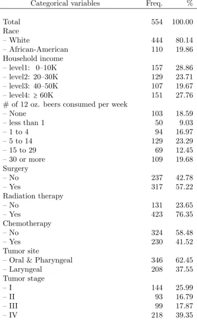
Table 3.1: Descriptive statistics of predictors in the CHANCE study

Categorical variables Freq. %

Total 554 100.00

Race

– White 444 80.14

– African-American 110 19.86

Household income

– level1: 0–10K 157 28.86

– level2: 20–30K 129 23.71

– level3: 40–50K 107 19.67

– level4: ≥60K 151 27.76

# of 12 oz. beers consumed per week

– None 103 18.59

– less than 1 50 9.03

– 1 to 4 94 16.97

– 5 to 14 129 23.29

– 15 to 29 69 12.45

– 30 or more 109 19.68

Surgery

– No 237 42.78

– Yes 317 57.22

Radiation therapy

– No 131 23.65

– Yes 423 76.35

Chemotherapy

– No 324 58.48

– Yes 230 41.52

Tumor site

– Oral & Pharyngeal 346 62.45

– Laryngeal 208 37.55

Tumor stage

– I 144 25.99

– II 93 16.79

– III 99 17.87

– IV 218 39.35

Continuous variables n mean std.dev min median max

Age at diagnosis 554 59.11 10.19 24.00 59.00 80.00

# of persons supported by household income 554 2.23 1.06 1.00 2.00 5.00

BMI 554 27.47 5.98 15.66 26.48 56.28

Total # of medical conditions reported 554 .92 1.10 .00 1.00 6.00

Time at 1st survey measurement (years) 209 .41 .45 .09 .28 3.55

Time at 2nd survey measurement (years) 500 1.85 .86 .44 1.81 3.91

Time at 3rd survey measurement (years) 353 3.49 .54 1.88 3.54 4.88

(56)

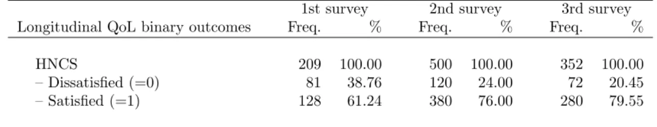
Table 3.2: Descriptive statistics of outcome variables in the CHANCE study

1st survey 2nd survey 3rd survey

Longitudinal QoL binary outcomes Freq. % Freq. % Freq. %

HNCS 209 100.00 500 100.00 352 100.00

– Dissatisfied (=0) 81 38.76 120 24.00 72 20.45

– Satisfied (=1) 128 61.24 380 76.00 280 79.55

Survival outcomes n mean std.dev min median max

min(Survival time, Censored time) (years) 554 3.07 1.04 .44 2.91 5.98

Freq. %

Censorship 554 100.00

– Alive 469 84.66

– Death 85 15.34

3.3 Models and Inference Procedure

3.3.1 Model formulation and notation

Longitudinal measurements are considered as the realizations of a certain marker pro-cess at finite time points, and we useY(t)to denote the value of such a marker process at timet. We letT be survival time, and suppose that the survival timeT is possibly right censored and the right-censoring time is missing at random. Suppose a set of n

subjects are followed over an interval [0, τ], where τ is the study end time. Denote

bi, i=1, . . . , n, as a vector of subject-specific random effects of dimension db and bi’s

are mutually independent and identically distributed from a multivariate normal with mean zero and covariance matrix Σb.

Given the random effects bi, the observed covariates, and the observed outcome

Choi_unc_0153D_12105.pdf

Statistical Methods for Joint Analysis of

Survival Time and Longitudinal Data

Abstract

Acknowledgments

Table of Contents

List of Tables

List of Figures

Chapter 1

INTRODUCTION

1.1

Joint Analysis for Survival Time and Longitudinal

Cate-gorical Measurements of Quality of Life in Head and Neck

Cancer Patients

1.2

Joint Modeling of Survival Time and Longitudinal

Out-comes with Flexible Random Effects

1.3

Penalized Likelihood Approach for Joint Analysis of

Sur-vival Time and Longitudinal Outcomes

Chapter 2

LITERATURE REVIEW

2.1

Failure Time Models

2.1.1

Univariate failure time model

2.1.2

Correlated failure time model

2.2

Longitudinal Data Models and Methods

2.2.1

Generalized linear model with random effects

2.2.2

Maximum likelihood and conditional likelihood methods

2.3

Joint Models of Failure Time and Longitudinal Data

2.3.1

Failure time model with longitudinal covariates

2.3.2

Simultaneous model of failure time and longitudinal data

2.4

Penalized Quasi-Likelihood Approach

2.4.1

Penalized quasi-likelihood in generalized linear mixed

model

2.4.2

Bias correction in penalized quasi-likelihood

Chapter 3

JOINT ANALYSIS FOR SURVIVAL

TIME AND LONGITUDINAL

CATEGORICAL MEASUREMENTS OF

QUALITY OF LIFE IN HEAD AND

NECK CANCER PATIENTS

3.1

Introduction

3.2

The CHANCE Study

3.3

Models and Inference Procedure

3.3.1

Model formulation and notation