Preventing NEETs During the Great Recession –
The Effects of a Mandatory Activation Program
for Young Welfare Recipients
∗
Emile Cammeraat
†Egbert Jongen
‡Pierre Koning
§October 2017
Abstract
We study the impact of a mandatory activation program for young welfare recipients in the Netherlands. Introduced at the end of 2009, the goal of the program was to prevent so-called NEETs (individuals not in employment, ed-ucation or training). We use a large administrative data set for the period 1999–2012 and employ differences-in-differences and regression discontinuity to estimate the effects of the reform. We find that the reform reduced the number of NEETs on welfare, increased the number of NEETs not on wel-fare, and had no effect on the overall number of NEETs. Our finding that the reform did not reduce the total number of NEETs contrasts with previous studies, which may be due to the fact that the reform took place during a severe economic recession.
JEL codes: C21, H31, J21
Keywords: NEETs, mandatory activation programs, differences-in-differences,
regression discontinuity
∗We are grateful to Ineke Bottelberghs, Marina Pool and Mirthe Bronsveld-de Groot of Statistics
Netherlands for the data on participation in mandatory activation programs by young welfare recipients. Furthermore, we are grateful for comments and suggestions by Leon Bettendorf, Richard
Blundell, Matz Dahlberg, Sander Gerritsen, Bas Jacobs, Max van Lent, Dani¨el van Vuuren and seminar and conference participants at Leiden University, CPB Netherlands Bureau for Economic
Policy Analysis, the IIPF 2016 Doctoral School in Mannheim, the IIPF 2016 Conference in South Lake Tahoe, EALE 2016 in Ghent, NED 2016 in Amsterdam, LAGV 2017 in Aix-en-Provence and
the RWI-GIZ Conference ‘What Works? The Effectiveness of Youth Employment Programs’ 2017 in Berlin. Remaining errors are our own.
†Leiden University. Corresponding author. Department of Economics, Steenschuur 25, 2311
ES, Leiden, The Netherlands. E-mail: [email protected].
‡CPB Netherlands Bureau for Economic Policy Analysis and Leiden University. E-mail:
§Leiden University, VU University Amsterdam, Tinbergen Institute and IZA. E-mail:
1
Introduction
Individuals not in employment, education or training (NEETs) are a major policy concern, in particular during periods of recession. NEET rates have not recov-ered yet from the Great Recession, making them a prime concern for the European Commission (Carcillo et al., 2015). Recently, President Juncker of the European Commission stated in his 2016 State of the Union speech that he wants to “continue to roll out the Youth Guarantee across Europe, improving the skillset of Europeans and reaching out to regions and young people most in need.” (European Commis-sion, 2016) This increased policy attention for reducing the number of NEETs is accompanied with a trend towards stricter conditions for receiving welfare benefits; via e.g. the imposition of job search requirements and/or by making welfare benefits receipt conditional on participation in so-called work-learn programs. Prominent ex-amples of such policies that are targeted at young unemployed individuals include the New Deal for Young People in the UK and the Jobs Corp in the US (Kluve, 2014). Previous studies have found that stricter conditionality of welfare benefits de-creases welfare claims and inde-creases employment rates (Blundell et al., 2004; Hernæs et al., 2016; Dahlberg et al., 2009; Bolhaar et al., 2016).
In this paper, we study the effects of a mandatory activation program for young
individuals during a severe economic recession. Specifically, we study the WIJ (Wet
Investeren in Jongeren, Work Investment Act for Young Individuals) reform, in-troduced in the Netherlands at the end of 2009, just after the start of the Great Recession. The reform targeted individuals up to and including 26 years of age. The goal of the WIJ reform was to reduce the number of young NEETs. To this end, welfare benefits were made conditional on participation in work-learn programs. We consider the effects of the WIJ reform on a large number of outcome variables: NEETs claiming welfare benefits, NEETs not claiming welfare benefits, the overall NEETs rate, the employment rate and the enrollment rate in education.
We use a large administrative data set called the Labour Market Panel (
Arbei-dsmarktpanel) of Statistics Netherlands (2015). The Labour Market Panel tracks 1.2 million individuals over the period 1999–2012 and contains a large set of labour market outcomes and a large number of individual and household characteristics. We use differences-in-differences and regression discontinuity to estimate the causal effects of the WIJ reform. Our base treatment group consists of individuals 25-26
years of age, and our base control group consists of individuals 27-28 years of age. A key challenge in the empirical analysis is to control for potentially different time effects between the treatment and control group, due to e.g. differential trends or different business cycle responses (Bell and Blanchflower, 2011). In our preferred specification we therefore include demographic controls, a full set of unemployment-age dummies, unemployment-age-specific trends and control-specific trends. We also present an extensive placebo analysis, including placebo treatment dummies for the years just before the reform and placebo treatment dummies for the earlier economic downturn in 2002–2004.
Our main findings are as follows. First, we find that the reform had a statistically significant large negative effect on the number of young NEETs claiming welfare benefits of –24%. Second, the reform had only a small and statistically insignificant effect on the total number of young NEETs. The reform pushed young individuals out of welfare, but did not increase the number of young individuals in employment or education. Third, our analysis shows that controlling for differential trends in a differences-in-differences analysis may be important for some outcome variables, like the enrollment rate in education, when studying a reform that targets young individuals and using somewhat older individuals as a control group.
Our paper relates to a number of studies that consider the effects of mandatory
activation programs for young individuals.1 Blundell et al. (2004) use area-based
piloting and age-related eligibility rules to identify the employment impact of a mandatory job search programme in the UK, the New Deal for Young People. They find that the program increased the probability to find employment by about five percentage points. Persson and Vikman (2010) analyze entry and exit effects of a welfare reform in Sweden where city districts in Stockholm implemented mandatory activation programs at different rates. They find that the reform reduced welfare participation and increased employment rates of younger individuals, particularly those born in non-Western countries. Hernæs et al. (2016) exploit a geographically differentiated implementation of conditionality of welfare benefits for Norwegian
1Our analysis also contributes to a broader literature on the effect of training programs targeted
at the youth. The overall success rate of programs on employment and wage earnings is found to be small, see e.g. a recent meta-analysis by Kluve et al. (2016). According to Kluve et al.
(2016), one of the key determinants of success is that programs consist of a comprehensive set of interventions, like training, counselling, intermediation and private sector incentives.
youth and find that stricter conditionality reduces welfare claims and increases high school completion rates. These analyses suggest that the combination of welfare conditionality and welfare-to-work programs can reduce the number of NEETs and promote employment and enrollment in education among young individuals.
We make the following contributions to this literature. First, we show that stricter conditionality combined with welfare-to-work programs does not always in-crease employment or enrollment in education. Indeed, we find that for the WIJ reform there was no effect on the number of young NEETs. The main effect of the reform was simply to push young individuals out of welfare. This is likely to be due to the state of the business cycle, as the reform clashed head on with the start of the Great Recession, during which it was hard for people, in particular young individuals, to find a job. Second, we consider all potential outcome states, not only NEETs on welfare but also NEETs not on welfare, and the enrollment in education next to employment. Indeed, our analysis for young individuals in the treated group shows that when looking at the effects on the employment rate, it is important to study changes in the enrollment rate in education as well. Third, we use an excep-tionally large and long data set, that allows us to study and account for differential trends and test for differences in business cycle responses across age groups and in an earlier economic downturn.
The outline of the paper is as follows. Section 2 describes the institutional setting and the main features of the reform. Section 3 discusses the empirical methodology. Section 4 discusses the data set and gives descriptive statistics. In Section 5 we then present graphical evidence, the estimation results and a number of robustness checks. Section 6 discusses our findings and concludes. An appendix contains supplementary material.
2
Institutional setting and the reform
Young NEETs are a policy concern in all OECD countries. However, there is con-siderable variation in the share of NEETs among the young across OECD countries, and the extent to which the share of NEETs has risen (or fallen) during the Great Recession, see Table 1. Panel A gives indicators for individuals 20–24 years of age, and panel B gives indicators for individuals 25–29 years of age. The Netherlands has one of the lowest NEETs shares among OECD countries, in 2015 only 8.9% of
20–24 year olds in the Netherlands were NEETs.2 Compared to 2005, there has
been a moderate rise in the share of NEETs in the Netherlands. The low share of NEETs in the Netherlands is mirrored by the high share of 20–24 year olds that are in education, as well as by the high share of 20–24 year olds that are employed, whereas the share of unemployed 20–24 year olds is relatively low, see again Table
1.3 Also regarding individuals 25–29 years of age, the Netherlands scores relatively
favorable in terms of a low NEETs rate, a high enrollment rate in education and participation rate in employment rate, and a relatively low unemployment rate.
In the Netherlands, welfare benefits form a safety net that is provided by munic-ipalities to support unemployed individuals who are not, or are no longer, entitled to other types of social insurance benefits like unemployment insurance. The vast majority of new welfare recipients consists of individuals with insufficient work his-tory for entitlement to unemployment insurance. Indeed, in 2014, only 22% of all new welfare recipients consisted of unemployed workers who exhausted their unem-ployment insurance benefits (UWV, 2014). Welfare benefits are means-tested and
assets-tested.4 The level of welfare benefits differs across household types and age
groups. In 2008, before the start of the WIJ reform, welfare benefits ranged from 220 euro per month for singles of 18–20 years of age to 1,320 euros per month for couples with children (Ministry of Social Affairs and Employment, 2008).
The Work Investment Act for Young Individuals (Wet Investeren in Jongeren,
WIJ) came into force in October 2009 as a consequence of increased policy atten-tion for NEETs and welfare dependency. The reform was designed before the start of the Great Recession, but the implementation was after the start of the Great Recession (September 2008). The WIJ reform aimed at activating the young, as well as fostering their human capital formation. The WIJ stipulated that for in-dividuals below the age of 27, entitlement to welfare benefits was conditional on
participation in a mandatory activation program.5 These programs were defined
2In 2015, the only country in the OECD with a lower share of NEETs was Iceland (6.6%).
3The shares of individuals in education and individuals in employment add up to more than
100% because individuals in education can be employed, and employed individuals can also be in education.
4For single individuals, net worth should not exceed 5,765 euro. For households with more
persons, net worth should not exceed 11,895 euro.
5The WIJ contains many elements that are similar to the New Deal program for younger
individuals in the UK (Wilkinson, 2003; Blundell et al., 2004; Dorsett, 2006).
Table 1: NEETs – An international perspective
NEETs-to- Education-to- Employment-to-
Unemployment-to-population rate population rate population rate population rate
Year 2005 2015 2015 2015 2015
Panel A: Individuals 20–24 years of age Continental Europe
Netherlands 8.1 8.8 57.7 69.4 6.7
Belgium 18.3 15.8 45.3 42.0 9.8
France 17.8 20.9 44.4 46.2 14.2
Germany 18.7 9.3 54.4 64.3 5.1
Scandinavia
Denmark 8.3 12.4 59.1 63.4 7.6
Finland 13.0 18.3 47.8 52.5 14.7
Norway 9.6 10.2 42.1 66.6 5.8
Sweden 13.4 11.8 46.0 56.4 13.0
Anglo-Saxon countries
Australia 11.6 13.1 44.5 71.5 7.3
Canada 14.4 14.4 41.6 64.7 8.3
United Kingdom 16.8 15.6 33.8 65.3 8.2
Unites States 15.5 15.8 38.5 64.1 6.5
OECD average 17.3 16.9 44.8 53.4 9.9
Panel B: Individuals 25–29 years of age
Continental Europe
Netherlands 10.7 12.1 20.8 82.2 5.7
Belgium 17.7 20.2 8.5 74.4 11.0
France 19.8 23.4 8.5 72.1 12.5
Germany 21.2 12.8 20.8 77.9 5.0
Scandinavia
Denmark 11.6 15.2 30.4 73.8 7.9
Finland 14.0 18.2 26.9 70.2 10.1
Norway 12.3 14.0 14.6 77.1 5.2
Sweden 10.0 10.8 25.1 75.6 8.7
Anglo-Saxon countries
Australia 15.4 15.5 19.1 78.5 4.4
Canada 15.7 17.6 12.8 76.7 7.0
United Kingdom 16.6 16.2 12.7 79.4 5.0
Unites States 18.1 20.0 13.2 75.4 4.7
OECD average 19.0 19.3 16.3 73.5 9.4
Notes: Using data from OECD (2016a), OECD (2016b) and OECD (2016c). The education-to-population rate is the enrollment in education divided by the relevant age population. The unemployment-to-population rate is calculated as
Figure 1: Participation rate of individuals on welfare in activation programs
0.0 0.1 0.2 0.3 0.4 0.5 0.6 0.7 0.8 0.9 1.0
2009 2010 2011 2012 2013 2014
25-26 27-28
Source: Statistics Netherlands (personal communication). The solid black line and the dashed red line give the share of individuals on welfare participating in an activation program in our preferred control group (27–28 years
of age) and our main treatment group (25–26 years of age), respectively.
as work-learn offers and consisted of public employment programs, apprenticeships and internships. Any wage earnings in these programs were supplemented up to the level of welfare benefits. As Figure 1 shows, the WIJ increased the coverage rate of activation programs for young welfare recipients in our preferred treatment group (individuals 25–26 years of age) from around 80% in January 2009 to almost 90% in 2011. Hence, the reform restricted the discretionary room of caseworkers in administering welfare benefits and work-learn offers.
The WIJ applied to all new entrants into welfare from October 2009 onwards. However, as the enactment of the WIJ implied a substantial increase in the workload for municipalities, municipalities were given 9 additional months – until July 2010 – to increase coverage of the WIJ to 100% of the pre-existing stock of welfare recipients. Figure 1 suggests that in the end it took until January 2011 for the WIJ to achieve
its largest coverage.6
6This is consistent with the numbers presented in Leenheer et al. (2011), who calculate that
about 70% of the WIJ applications received a work-learn offer in 2010, 11% received welfare benefits
without a work-learn offer, and the remaining 19% did not receive welfare benefits.
To get a better understanding of the implementation of the WIJ reform at the local level, we interviewed policymakers and caseworkers in the city of Amsterdam that were involved in the design and implementation of the WIJ. In Amsterdam, the majority of work-learn offers were provided by retail companies, local industries and welfare-to-work organizations. The respondents in our interviews stressed that some aspects of the WIJ were already common practice in Amsterdam. That is, ap-prenticeships, internships and public employment programs were already provided for individuals up to 23 years of age (Board of Amsterdam, 2009). In effect, in Ams-terdam the WIJ reform thus implied the extension of these programs to individuals with 24–26 years of age, together with the imposition of welfare conditionality for all young individuals below the age of 27. In our empirical analysis, we focus on the group of individuals 25–26 years of age, but we also consider the effects for younger age groups.
Finally, next to the WIJ reform, there were two other reforms relevant for our analysis that took place in January 2012. First, the government replaced the manda-tory acceptance of work-learn offers with ’work-first’ arrangements. Specifically, the government introduced an initial one-month ‘job-search period’ during which indi-viduals younger than 27 years of age did not receive welfare benefits. This may explain the small drop in the participation rate in activation programs in January 2012, and the larger drop in January 2013, see Figure 1. Second, adult children liv-ing at home were no longer eligible to welfare benefits when they lived in a household in which first-degree relatives had sufficient income or assets (the ‘household-income test’). In the empirical analysis we also consider treatment effects by individual years, the treatment effect on the probability of being an adult child living at home and the treatment effects for the subgroup of adult children living at home.
3
Empirical methodology
We use differences-in-differences (DD) and regression discontinuity (RD) to estimate
the effects of the WIJ reform on a number of outcome variables.7,8
7For a general introduction to the differences-in-differences and regression discontinuity
method-ologies see e.g. Angrist and Pischke (2009).
8Our preferred method is differences-in-differences because this gives us an average treatment
effect for a larger group than the local average treatment effect of regression discontinuity.
3.1
Differences-in-differences
We stated earlier that the reform was targeted at individuals up to 27 years of age and started in October 2009. A key assumption of the DD approach is common time effects for the treatment and control group (in the absence of the reform). In this context, our preferred model focuses on a treatment group consisting of individuals 25–26 years of age and a control group consisting of individuals 27–28 years of age. We will also consider the treatment effects for younger individuals, but we will show that changes in the enrollment in education complicate the analysis for this group (young individuals in the treated group have a choice of staying in education, while this is hardly a choice for individuals in the control group). The age variable is measured on the 1st of October of each year, and the outcome variables are averages for October each year.
As outcome variables we consider (i) the ‘participation rate’ in NEETs, defined
as not being in employment or education9, (ii) the participation rate in NEETs on
welfare, (iii) the participation rate in NEETs not on welfare, (iv) the employment rate, and (v) the enrollment rate in education. The participation rate in NEETs, the employment rate and the enrollment rate in education sum to one, but we analyse them independently.
For all these outcome variables we estimate a linear probability model (Angrist
and Pischke, 2009). Let yiat be a dummy variable that is 1 if individual i in age
group a is ‘participating’, ’employed’ or ‘enrolled’ in period t. In our most
ex-tensive specification, we regress the outcome variable on a set of year fixed effects
(αt), age fixed effects (βa), age-specific trends with coefficients (γa), an interaction
term between age and the unemployment rate (ut) with age-specific coefficientφa, a
set of demographic controlsXi (gender and ethnicity) with coefficients µx, a set of
demographic-control-specific trends with coefficients ψx, a treatment effect (DDat)
for individuals in the treatment group with ageain a given yeartin the post-reform
thermore, we may be concerned that welfare recipients or their caseworkers might anticipate the 27th birthday of the welfare recipient, when participation in work-learn arrangements is no longer
obligatory, or that participation in work-learn arrangements may continue after the 27th birthday of the welfare recipient, although a robustness analysis where we leave out observations close to
the threshold using a so-called donut-RD design yields similar results as the base RD specification
with these observations included.
9Similar to the OECD, we do not observe participation in training programs in our dataset.
period with coefficientδa, and an error term (iat):
yiat =αt+βa+γat+φaut+Xi0µx+Xit0 ψxt+δa,tDDat+iat. (1)
We are primarily interested in the treatment coefficients δa,t. We include an
inter-action term between age and the unemployment rate to allow for different business cycle responses across age groups (Bell and Blanchflower, 2011). Furthermore, we include age-specific and demographic-control-specific trends to allow for trend
dif-ferences.10
In an extension to this model, we add placebo treatment dummies for the pre-reform years 2008 and 2009. The coefficients on these placebo treatment dummies are informative about potential remaining differential time effects between the treat-ment and control groups, for example because of changes in group specific trends or differences in business cycle responses not captured by the age-specific unemploy-ment terms, and also about potential anticipation effects of the reform. In addition, we will allow for time trends that vary across all ages in our sample.
Finally, to allow for correlation in the error terms at a higher level than the individual and over time, we use cluster-robust standard errors (Bertrand et al., 2004; Donald and Lang, 2007). We cluster the standard errors by year of birth interacted with the region where the individual is living. This results in 216 clusters in our base DD specification, which is deemed sufficiently large by Angrist and Pischke (2009) to use the large sample properties of the estimator.
3.2
Regression discontinuity
In the RD approach we estimate the impact of the policy by comparing differences in the outcome variables for individuals that are just younger than the cutoff of 27 years that determines treatment by the WIJ reform with individuals that are just older than this cutoff. A key assumption here is that in the absence of the reform, the outcome variables are a smooth function in age, and the reform introduces a discontinuity in these relations.
Similar to the DD approach, we specify outcomes in linear probability models. In
our preferred specification, we regress participation statusyiat on a year fixed effect
10We have 10 years of pre-reform data to estimate the coefficients on these trends.
(βt), age in months ait (recentered11, with coefficient βa), an interaction term that
captures the additional effect of age when the person is younger than the cutoff a0
(with coefficientβa<a0) to allow for a different slope to the left of the discontinuity, a
treatment effect if the age of the person is below 27 (with coefficientβRD) capturing
the discontinuity, individual characteristicsXi and an error term it:12
yit =βt+βaait+βa<a01(ait < a0)ait+βRDRDit+X0
iµx+it. (2)
Our primary interest is in βRD, which measures the size of the discontinuity in
the relationship between the outcome variable and age due to the policy. For an accurate measurement of the discontinuity it is important to get a precise estimate of the relation between age and the outcome variables around the discontinuity. In
the RD analysis we therefore use month of birth relative to the discontinuity13as the
running variable. Since the identification in the RD approach comes from differences in month of birth, we cluster standard errors by month of birth (with persons born in the same month but in different years in different clusters). This generates 72 clusters in the base specification, again deemed large enough to use the large sample properties of the estimator (Angrist and Pischke, 2009).
In an extension of the RD analysis we consider a ‘difference-in-discontinuity’ setup, using both the pre- and post-reform data – see e.g. the analysis of Bettendorf et al. (2014). This specification may be relevant if the age cutoff of 27 years of age cannot be uniquely linked to the WIJ reform but that other pre-existing policies use a similar cutoff. To test for this possibility, we use observations both before and after the policy reform to control for a potential discontinuity before the reform. In
this specification we include a treatment effect γP RD that captures the pre-reform
discontinuity, and an additional treatment effect for the post-reform discontinuity
relative to the pre-reform discontinuityγDRD. In the specification below, the
discon-tinuity before the reform equalsγP RD and the discontinuity after the reform equals
11Age is recentered so that individuals that have turned 27 in September have a value of 1, they
are the first age group to the ‘right’ of the discontinuity.
12We also esitmated models with a quadratic term in age, and with a different quadratic term
in age to the left of the threshold. The estimated discontinuities are similar to the results of our
preferred specification (available on request).
13The exact date of birth during the month is not available in our data set.
γP RD+γDRD:
yit = γt+γaait+γa2(ait)2+γa<a01(ait < a0)ait
+γP RDPRDit+γDRDDRDit+Xi0ν+υit, (3)
where for the same reasons as in the RD analysis we use age measured in months relative to the discontinuity as the running variable, and we cluster the standard errors by month of birth.
4
Data
We use data from the Labour Market Panel (Arbeidsmarktpanel) of Statistics
Nether-lands (2015). The Labour Market Panel is a large and rich household panel data
set, tracking 1.2 million individuals over the period 1999–2012.14 We use the years
1999–2009 as the pre-reform years, and 2010–2012 as the treatment years.
To ensure that the treatment and control groups are sufficiently similar, we limit the sample to individuals 25–28 years of age. As stated earlier, our preferred treatment group consists of individuals 25–26 years of age, and our main control
group consists of individuals 27–28 years of age.15
The outcome variables are based on the social-economic classification (SEC) variable in the Labour Market Panel. The SEC variable classifies individuals ac-cording to their main source of income, where individuals in education are always classified as being in the state of education (even if their wage income is larger than their study grant) and individuals with profit income are always classified as being self-employed (even if their wage income exceeds their profit income). According to the SEC individuals can be in the following states: (1) employee, (2) owner of closely-held company, (3) self-employed, (4) other type of employment, (5) on un-employment insurance, (6) on welfare benefits, (7) on disability or sickness benefits,
14For a limited number of variables, not used in this study, the data set also contains data for
2013.
15In the empirical analysis we show that business-cycle responses of the larger group of 20–26
years of age are not similar for all outcome variables, so that the assumption of common time effects does not hold.
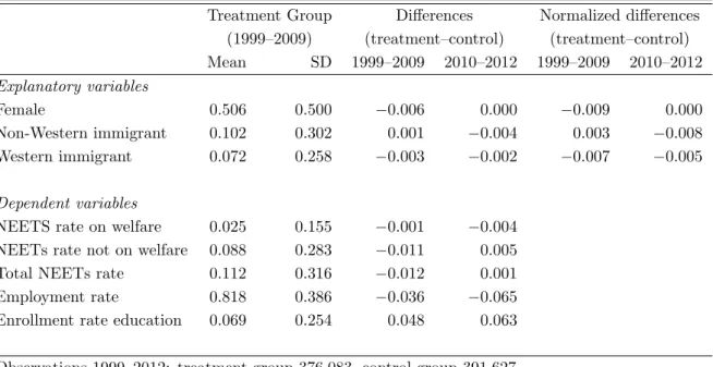
Table 2: Descriptive statistics treatment and control group in sample for estimations
Treatment Group Differences Normalized differences
(1999–2009) (treatment–control) (treatment–control)
Mean SD 1999–2009 2010–2012 1999–2009 2010–2012
Explanatory variables
Female 0.506 0.500 −0.006 0.000 −0.009 0.000
Non-Western immigrant 0.102 0.302 0.001 −0.004 0.003 −0.008
Western immigrant 0.072 0.258 −0.003 −0.002 −0.007 −0.005
Dependent variables
NEETS rate on welfare 0.025 0.155 −0.001 −0.004
NEETs rate not on welfare 0.088 0.283 −0.011 0.005
Total NEETs rate 0.112 0.316 −0.012 0.001
Employment rate 0.818 0.386 −0.036 −0.065
Enrollment rate education 0.069 0.254 0.048 0.063
Observations 1999–2012: treatment group 376,083, control group 391,627.
Source: Own calculations using the Labour Market Panel (Statistics Netherlands). Treatment group: individuals 25–26 years of age. Control group: individuals 27–28 years of age. Normalized differences are mean differences divided by the
square root of the sum of the variances (see Imbens and Wooldridge, 2009).
(8) on retirement benefits, (9) on other social insurance, (10) in education with in-come, (11) in education without inin-come, (12) without income. We count individuals in states (1)-(4) as employed, in states (10) and (11) as in education, and in states (5)-(9) and 12) as NEETs. Within the state of NEETs we count individuals in state (6) as NEETs on welfare and individuals in states (5), (7)-(9) and (12) as NEETs not on welfare. As demographic control variables we include gender and ethnicity (native/non-Western immigrant/Western immigrant).
Table 2 gives descriptive statistics for our treatment group, along with the dif-ferences and normalized difdif-ferences (for the demographic control variables) with the control group in the pre- and the post-reform period. The differences in the demo-graphic control variables gender and ethnicity are small, and the same is true for the so-called normalized differences (mean differences divided by the square root of the sum of variances). Imbens and Wooldridge (2009) argue that these normalized
differences are an informative way to check if the treatment and control group have sufficient overlap in the covariates. As a rule of thumb they suggest that when the normalized difference exceeds a value of .25, linear regression becomes sensitive to the specification. The normalized differences for gender and ethnicity stay well be-low .25. Furthermore, the differences in the demographic control variables hardly change from the pre- to the post-reform period. Hence, there is no indication of
differential changes in the composition of the treatment and control group.16
Table 2 also presents descriptive statistics for the outcome variables. The NEETs rate on welfare in the treatment group is very similar to the control group in the pre-reform period, but drops somewhat for the treatment group relative to the con-trol group in the post-reform period, suggesting a negative treatment effect on this outcome variable. The NEETs rate not on welfare is also quite similar for the treat-ment and control group before the reform, though somewhat lower for the treattreat-ment group than the control group. After the reform, the NEETs rate not on welfare is somewhat higher for the treatment group than the control group, suggesting a pos-itive treatment effect on this outcome variable. The total NEETs rate again is quite similar for the treatment and control group before the reform, though again somewhat lower for the treatment group than the control group. After the reform, the total NEETs rate of the treatment and control group are comparable, which suggests a positive treatment effect for the total NEETs rate. The employment rate is higher in the control group in the pre-reform period, and the difference in the employment rate becomes more negative in the post-reform period, suggesting a (counterintuitive) negative treatment effect on the employment rate. Finally, the enrollment rate in education shows the mirror image of the employment rate. The enrollment is higher in the treatment group than the control group in the pre-reform period, and the difference becomes bigger in the post-reform period, suggesting a positive treatment effect on the enrollment in education. However, these simple treatment effects do not account for differential trends between the treatment and control groups. These differential trends will turn out to be important for some outcome variables in the empirical analysis below.
16See also Figure A.3 in the Supplementary material.
5
Results
5.1
Differences-in-differences
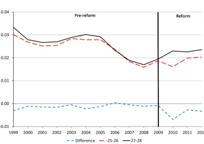
Figure 2 first presents graphical evidence on the treatment effects of the reform on the outcome variables. The solid black lines denote the control group (27–28 years of age), the dashed red lines denote the treatment group (25–26 years of age) and the dotted blue lines denote the difference between the treatment group and the control group. What is clear from these graphs, is that the NEETs rate on welfare moves very much in tandem for the treatment and control group in the pre-reform period, and there is a clear negative treatment effect in 2010, which subsequently becomes smaller in 2011 and 2012. The graphs also make clear that there are trend differences between the treatment and control group for the other outcome variables. Hence, accounting for these differential trends will be important to isolate the treatment effect of the reform. This also makes it hard to eyeball potential treatment effect for these outcomes.
Table 3 gives the base regression results for the different outcome variables, using
a single treatment dummy for all years and both ages in the treatment group.17 First
consider the results for the NEETs rate on welfare. Column (1) shows the results of the basic DD setup, where we only include year dummies, a group dummy for each individual age group and a treatment dummy for the age group 25–26. This setup suggests a negative and statistically significant treatment effect of –0.30 percentage points. In column (2) we add demographic controls. Consistent with the observa-tion that there were hardly any composiobserva-tional changes in these characteristics, this hardly affects the estimated treatment effect. Still, the treatment effect is now only statistically significantly different from zero at the 10% level. In column (3) we next add interaction dummies for age and the national unemployment rate, to allow for a potential different business-cycle response by age. Again, this yields a treatment effect that is very similar to columns (1) and (2). In column (4) we allow for age-specific trends, this leads to a somewhat larger treatment effect in absolute terms (more negative) of –0.43 percentage points. Finally, column (5) with our preferred specification shows that the inclusion of demographic-control specific trends gives a treatment effect that is very similar to the treatment effect in column (4), but
17Full regression results can be found in Table A.1 in the Supplementary material.
Figure 2: Differences-in-differences in outcome variables of individuals aged 25-26 and 27-28: 1999–2012
(a) NEETs rate on welfare
-0.01 0.00 0.01 0.02 0.03 0.04
1999 2000 2001 2002 2003 2004 2005 2006 2007 2008 2009 2010 2011 2012
Difference 25-26 27-28
Pre-reform Reform Pre-reform Reform
(b) NEETs rate not on welfare
-0.02 0.00 0.02 0.04 0.06 0.08 0.10 0.12
1999 2000 2001 2002 2003 2004 2005 2006 2007 2008 2009 2010 2011 2012 Difference 25-26 27-28
Pre-reform Reform Pre-reform Reform
(c) Total NEETs rate
-0.04 -0.02 0.00 0.02 0.04 0.06 0.08 0.10 0.12 0.14 0.16
1999 2000 2001 2002 2003 2004 2005 2006 2007 2008 2009 2010 2011 2012 Difference 25-26 27-28
Pre-reform Reform Pre-reform Reform
(d) Employment rate
-0.20 0.00 0.20 0.40 0.60 0.80 1.00
1999 2000 2001 2002 2003 2004 2005 2006 2007 2008 2009 2010 2011 2012 Difference 25-26 27-28
Pre-reform Reform Pre-reform Reform
(e) Enrollment rate in education
0.00 0.02 0.04 0.06 0.08 0.10 0.12
1999 2000 2001 2002 2003 2004 2005 2006 2007 2008 2009 2010 2011 2012 Difference 25-26 27-28
Pre-reform Reform Pre-reform Reform
Notes: Own calculations using the Labour Market Panel (Statistics Netherlands). The solid black lines denote the control group (27–28 years of age), the dashed red lines denote the treatment group (25–26 years of age) and
the dotted blue lines denote the difference between the treatment group and the control group. NEETs rates are
individuals not in employment or education relative to the relevant age population, employment rates are individuals
in employment relative to the relevant age population and enrollment rates in education are individuals in education
17
Table 3: Differences-in-differences: base regression results
(1) (2) (3) (4) (5)
NEETs rate on welfare −0.0030∗∗ −0.0028∗ −0.0032∗ −0.0043∗ −0.0045∗∗
(0.0015) (0.0015) (0.0017) (0.0023) (0.0021)
NEETs rate not on welfare 0.0156∗∗∗ 0.0158∗∗∗ 0.0135∗∗∗ 0.0058 0.0059∗
(0.0023) (0.0025) (0.0027) (0.0036) (0.0034)
Total NEETs rate 0.0126∗∗∗ 0.0130∗∗∗ 0.0103∗∗∗ 0.0016 0.0014
(0.0031) (0.0035) (0.0038) (0.0052) (0.0048)
Employment rate −0.0288∗∗∗ −0.0295∗∗∗ −0.0210∗∗∗ −0.0023 −0.0023
(0.0055) (0.0048) (0.0052) (0.0067) (0.0066)
Enrollment rate in education 0.0162∗∗∗ 0.0164∗∗∗ 0.0106∗∗ 0.0007 0.0009
(0.0041) (0.0039) (0.0042) (0.0052) (0.0051)
Demographic controls NO YES YES YES YES
Unemployment-age interaction terms NO NO YES YES YES
Age-specific trends NO NO NO YES YES
Control-specific trends NO NO NO NO YES
Observations 767,710 767,710 767,710 767,710 767,710
Clusters 216 216 216 216 216
Notes: * denotes significant at the 10% level, ** at the 5% level and *** at the 1% level. Sample period 1999–2012. Treatment group: individuals 25–26 years of age. Control group: individuals 27–28 years of age. Cluster-robust standard errors in
paren-theses, clustered by year-of-birth*province (18*12=216 clusters), All specifications include age and year fixed effects. See Table
A.1 in the Supplementary material for the full regression results.
Table 4: Differences-in-differences: placebo’s and annual treatment effects
(1) (2) (3) (4) (5)
NEETs rate NEETs rate Total Employment Enrollment rate
on welfare not on welfare NEETs rate rate in education
Placebo 2008 −0.0023 0.0046 0.0022 −0.0025 0.0003
(0.0028) (0.0058) (0.0073) (0.0091) (0.0061)
Placebo 2009 −0.0023 0.0025 0.0002 −0.0019 0.0017
(0.0034) (0.0065) (0.0085) (0.0105) (0.0076)
Treatment 2010 −0.0086∗∗∗ 0.0111∗ 0.0025 −0.0006 −0.0019
(0.0030) (0.0060) (0.0078) (0.0102) (0.0073)
Treatment 2011 −0.0044 0.0094 0.0051 −0.0090 0.0039
(0.0032) (0.0062) (0.0081) (0.0111) (0.0082)
Treatment 2012 −0.0050 0.0037 −0.0013 −0.0026 0.0040
(0.0032) (0.0059) (0.0077) (0.0104) (0.0077)
Observations 767,710 767,710 767,710 767,710 767,710
Clusters 216 216 216 216 216
Notes: * denotes significant at the 10% level, ** at the 5% level and *** at the 1% level. Sample period 1999–2012. Treatment group: individuals 25–26 years of age. Control group: individuals 27–28 years of age. Cluster-robust
standard errors in parentheses, clustered by year of birth*province (18*12=216 clusters). All specifications include
now also statistically significant at the 5% level. The treatment effect in column (5) of –0.45 percentage points also suggests a sizable negative treatment effect on the NEETs rate on welfare of –24% relative to a baseline of 1.9 percentage points in the last pre-reform year (2009).
As noted before, accounting for trend differences between the treatment and control group is important for the other outcome variables. Considering the other outcome variables, we find rather similar treatment effects for the base DD specifica-tion in columns (1)-(3). Allowing for differential trends, however, has an important impact on the treatment effects, in particular for the employment rate and the en-rollment rate in education – as is shown in column (4). Again, the inclusion of demographic-control specific trends in column (5) results in very similar treatment effects as in column (4). Our preferred specification is in column (5), with results suggesting a positive treatment effect on the NEETs rate not on welfare, significant at the 10% level, and essentially no effect on the total NEETs rate. Also, there appears to be no effect on the employment rate and the enrollment rate in educa-tion. Hence, the reform seems to have pushed or kept the treated individuals out of welfare, but this did not result in more employment and/or enrollment in education. In Table 4, we take specification (5) of Table 3 and include placebo treatment dummies for the years 2008 and 2009. We also split the treatment dummy for 2010– 2012 into individual-year treatment dummies for 2010, 2011 and 2012. With this specification, we can both test for the robustness of our results and the evolution of the effects of the WIJ reform over time. We find coefficients on the placebo treatment dummies that are small and statistically insignificant for all outcome variables. The treatment dummy for 2010, the first year of the reform, is statistically significant and more negative than the combined dummy for 2010–2012 in Column (5) of Table 3. Indeed, the treatment effects for 2011 and 2012 are rather small and not statistically significant, consistent with the pattern we see in Figure 2. Hence, the effect seems to have faded rather quickly. Also for the NEETs rate not on welfare, most of the effect appears to be in 2010, after which the effect becomes smaller again. There is no statistically significant treatment effect for the total NEETs rate, the employment rate and the enrollment rate in education, also not when we consider individual treatment years.
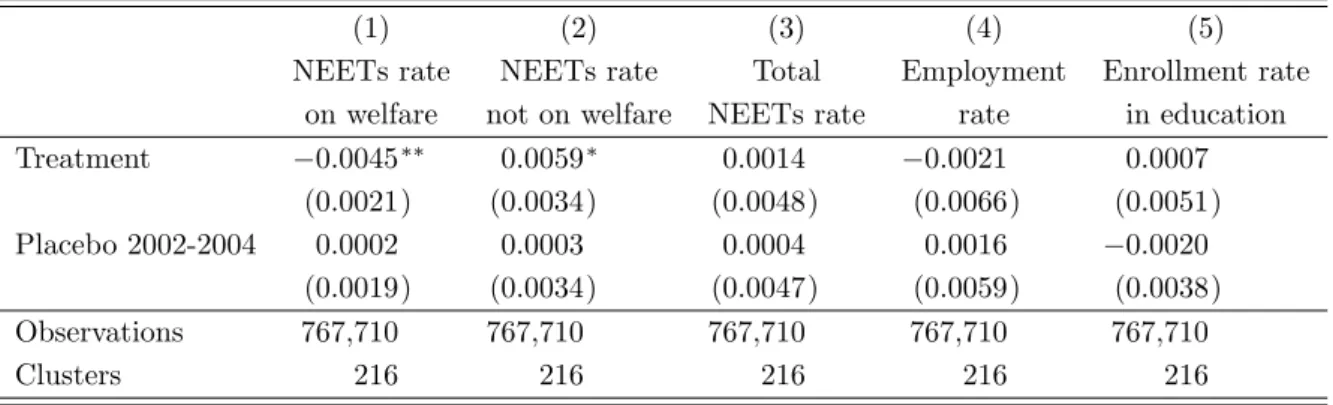
The Supplementary material contains a number of additional robustness analy-ses. In Table A.2 we perform an additional placebo analysis, and consider a placebo
treatment effect during the previous economic downturn, the years 2002–2004. The estimated placebo treatment effects are small and statistically insignificant, sug-gesting that the treatment and control groups did not respond differently to the economic downturn between 2002 and 2004. Table A.3 shows that the same is not true if we would consider the larger treatment group of individuals 20–26 years of
age.18 For this treatment group, the placebo treatment effect for the years 2002–
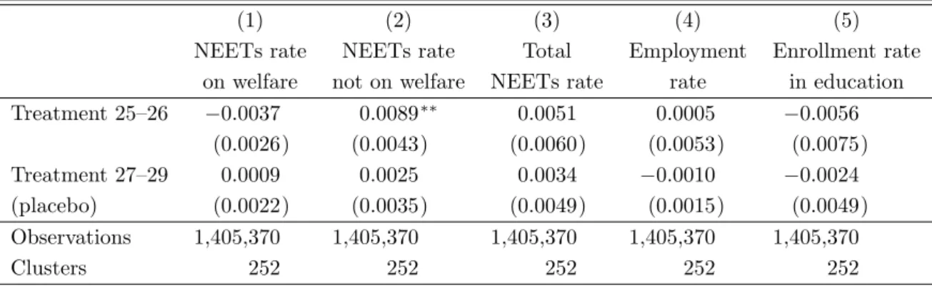
2004 is statistically significant for the employment rate and the enrollment rate in education. This justifies our decision to limit the treatment group in our main analysis to individuals 25–26 years of age. Next, one may worry that the reform created spillovers to the control group. In Table A.4 we address this concern and use individuals 29–30 years of age as an alternative control group, and introduce treatment dummies for individuals 25–26 years of age and individuals 27–28 years of age (our main control group). We find similar treatment effects for the preferred treatment group (25–26 years of age) and no statistically significant treatment ef-fects for our main control group (27–28 years of age). In Table A.5 we address the concern that treatment effects may persist as individuals age into the control group, another type of spillover effect that may bias our estimates. Here we use individ-uals 30–31 years of age as the control group, these individindivid-uals were never in the treatment group (during the WIJ treatment), and introduce treatment dummies for individuals 25–26 years of age and individuals 27–29 years of age. Again, the results for the preferred treatment group 25–26 years of age are similar to the base spec-ification, and the treatment effects for the control group of 27–29 years of age are statistically insignificant. Table A.7 shows that we obtain similar results when we narrow the treatment group down to individuals 26 years age and the control group to individuals 27 years of age. Finally, Table A.8 gives the results on the probability
of entering or exiting the different states.19 We then again consider results for our
most elaborate specification, including demographic controls, unemployment-age in-teraction terms, age-specific trends and demographic control-specific trends. These results suggest that most of the effect is via the exit from welfare, which is also
18Figure A.5 in the Supplementary material shows the outcome variables for this larger treatment
group over time. Table A.6 gives the regression results.
19Specifically, for entry the dependent variable equals 1 when, for each state, the current state is
1 and the previous state was a different state, and zero otherwise. For exit the dependent variable
equals 1 when, for each state, the current state is a different state than the previous state, and the previous state is 1, and zero otherwise.
statistically significant at the 5% level. The effect on the entry into welfare appears smaller. For the NEETs not on welfare we observe the opposite pattern, entry in the NEETs rate not on welfare increases, and there is hardly an effect on exit from the NEETs not on welfare. The effect on entry into and exit from NEETs as a whole is
small and statistically insignificant, consistent with the analysis of the stocks.20
The Supplementary material also presents the outcomes for other outcome vari-ables and for subgroups in our sample. Table A.9 considers the effects on the en-rollment rate in unemployment insurance (UI) and the enen-rollment rate in disability insurance (DI). We do not find a statistically significant effect on the enrollment rate in UI nor in DI. Table A.10 studies the treatment effect on being in a particular household type. We distinguish between adult children living at home, childless sin-gles, single parents and couples. We do not find a statistically significant treatment effect on being a particular household type. Table A.11 then studies the treatment effects by household type. The largest drop in the NEETs rate on welfare in ab-solute terms is for adult children living at home and single parents, –1.0 and –6.9 percentage points respectively. In percentages however, the drop for single parents is –22% (relative to the 2009 level), which is comparable to the average treatment effect over all household types. But for adult children living at home it is –45% (rel-ative to the 2009 level), much larger than the average drop. The effect for childless singles is comparable to the average over all household types, whereas the effect for couples is close to zero. The treatment effects for the other outcome variables are not statistically significant, the results hint at a drop in the total NEETs rate for adult children living at home, but not for the other household types. Table A.12 gives the results by gender and by ethnicity. The treatment effects (on e.g. the NEETs rate (not) on welfare) for males and females are similar to the base results. The treatment effects for natives appear somewhat smaller than the base results, whereas the results for immigrants are larger in absolute terms. But in percentage terms, the effects are much more comparable to the average, –29% for natives and –22% for immigrants for the NEETs rate on welfare (with no effect on the total NEETs rate). Finally, Table A.13 considers the treatment effects for provinces that had a relatively low and high pre-reform unemployment rate. The treatment effect appears to be smaller (about half) in the provinces which had a lower pre-reform
20The results also hint at a positive effect on the exit probability from education, but with
relatively large standard errors.
unemployment rate, though the difference between the treatment effect in low- and high-unemployment provinces is not statistically significant.
5.2
Regression discontinuity
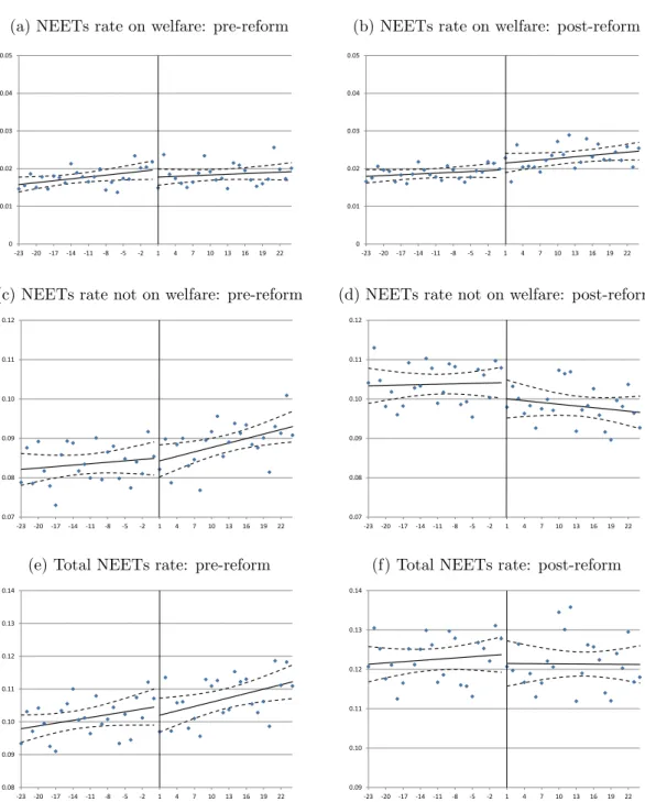
To shed light on the cutoff effects of the WIJ reform, Figure 3 shows the NEETs rate on welfare, the NEETs rate not on welfare and the total NEETs rate by month of birth relative to the discontinuity – and both for the pre-reform period (2007–2009,
left panels) and post-reform period (2010–2012, right panels).21 In the figures, value
averages are centered around the cutoff age of 27. The solid lines give the predictions from a RD regression without control variables, allowing for a separate intercept and slope on the left- and right-hand side of the discontinuity. The dashed lines give the corresponding 95% confidence intervals. These graphs suggest a small positive pre-reform discontinuity in the NEETs rate on welfare and a small negative post-reform discontinuity in the NEETs rate on welfare, and no pre-post-reform discontinuity for the NEETs rate not on welfare but a small positive post-reform discontinuity for the NEETs rate not on welfare. Finally, we observe a small and positive but similar pre- and post-reform discontinuity in the total NEETs rate.
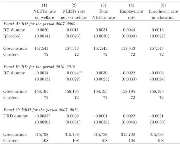
Consistent with these graphs, the RD estimation results that are presented in Table 5 indicate that treatment effects are small or insignificant for most outcome variables. In the table, the RD dummy captures a different intercept on the left hand side of the discontinuity, but we also allow for a different slope on the left hand side of the discontinuity and include year fixed effects and demographic control variables. We present results for the pre- and post-reform period, in Panel A and
B respectively.22 We find a small positive but statistically insignificant pre-reform
treatment effect for the NEETs rate on welfare, the NEETs rate not on welfare
21Similar plots for the employment rate and the enrollment rate in education are given in
Fig-ure A.7 in the Supplementary material section. These graphs show no statistically significant discontinuity in these outcome variables.
22Full regression results for the preferred RD specifications, for the pre- and post-reform period
respectively, can be found in Table A.16 and Table A.17 in the Supplementary material. Further-more, results for different RD specifications, for the pre- and post-reform period respectively, can
be found in Table A.14 and Table A.15 in the Supplementary material. Figure A.6 shows that there is no manipulation in the running variable (age of the child in months), and Figure A.8 and
A.9 show that there are also no discontinuities in the demographic control variables, either pre- or post-reform.
Figure 3: Pre-reform (2007–2009) and post-reform (2010–2012) outcome variables relative to the age threshold
(a) NEETs rate on welfare: pre-reform
0 0.01 0.02 0.03 0.04 0.05
-23 -20 -17 -14 -11 -8 -5 -2 1 4 7 10 13 16 19 22
(b) NEETs rate on welfare: post-reform
0 0.01 0.02 0.03 0.04 0.05
-23 -20 -17 -14 -11 -8 -5 -2 1 4 7 10 13 16 19 22
(c) NEETs rate not on welfare: pre-reform
0.07 0.08 0.09 0.10 0.11 0.12
-23 -20 -17 -14 -11 -8 -5 -2 1 4 7 10 13 16 19 22
(d) NEETs rate not on welfare: post-reform
0.07 0.08 0.09 0.10 0.11 0.12
-23 -20 -17 -14 -11 -8 -5 -2 1 4 7 10 13 16 19 22
(e) Total NEETs rate: pre-reform
0.08 0.09 0.10 0.11 0.12 0.13 0.14
-23 -20 -17 -14 -11 -8 -5 -2 1 4 7 10 13 16 19 22
(f) Total NEETs rate: post-reform
0.09 0.10 0.11 0.12 0.13 0.14
-23 -20 -17 -14 -11 -8 -5 -2 1 4 7 10 13 16 19 22
Notes: Own calculations using the Labour Market Panel (Statistics Netherlands). Age is recentered around the discontinuity (outcomes are measured in October, 1 is a person who has turned 27 in September). The solid lines
give the predictions from a RD regression without control variables, allowing for a separate intercept and slope on
the left and right hand side of the discontinuity. The dashed lines give the corresponding 95% confidence interval.
Table 5: Regression discontinuity: base regression results
(1) (2) (3) (4) (5)
NEETs rate NEETs rate Total Employment Enrollment rate
on welfare not on welfare NEETs rate rate in education
Panel A: RD for the period 2007–2009
RD dummy 0.0020 0.0011 0.0031 −0.0044 0.0013
(placebo) (0.0014) (0.0023) (0.0030) (0.0034) (0.0022)
Observations 157,543 157,543 157,543 157,543 157,543
Clusters 72 72 72 72 72
Panel B: RD for the period 2010–2012
RD dummy −0.0014 0.0044∗∗ 0.0030 −0.0022 −0.0008
(0.0013) (0.0022) (0.0023) (0.0030) (0.0024)
Observations 158,195 158,195 158,195 158,195 158,195
Clusters 72 72 72 72 72
Panel C: DRD for the period 2007–2012
DRD dummy −0.0033∗ 0.0032 −0.0001 0.0022 −0.0021
(0.0020) (0.0031) (0.0038) (0.0046) (0.0030)
Observations 315,738 315,738 315,738 315,738 315,738
Clusters 108 108 108 108 108
Notes: * denotes significant at the 10% level, ** at the 5% level and *** at the 1% level. Cluster-robust standard errors in parentheses, clustered by month of birth (72 cluster for the RD estimates, 108 clusters for the DRD
estimates). The RD parameter estimates are for the RD dummy capturing a different intercept on the left hand
side of the discontinuity, and also allow for a different slope on the left hand side of the discontinuity, include year
fixed effects and include demographic control variables. Full regression results for the RD specifications for the
period 2007–2009 and 2010–2012 can be found in Table A.16 and A.17 in the Supplementary material, respectively.
The DRD parameter estimates are for the DRD dummy capturing the difference in the different intercept on
the left hand side of the discontinuity from the period 2007–2009 to the period 2010–2012, and also allow for a
different slope on the left hand side of the discontinuity, a change in the different slope on the left hand side of the
discontinuity, include year fixed effects and include demographic control variables. Full regression results for the
and the total NEETs rate. Furthermore, the effect estimate of the RD dummy on education enrollment is small and insignificant in both the pre- and post-reform period. For the post-reform period we find a small but now negative treatment effect for the NEETs rate on welfare, though not statistically significant, a bigger positive and statistically significant treatment effect for the NEETs rate not on welfare, and a small positive treatment effect for the total NEETs rate that is similar to the effect in the pre-reform period (the post-reform treatment effect is somewhat larger for the employment rate and somewhat smaller for the enrollment rate in education). Panel C of Table 5 then gives the coefficient on the ‘difference-in-discontinuity’ dummy, which is very close to the difference in the discontinuity between the pre- and
post-reform period.23 The results are similar to the DD analysis. There is negative
treatment effect on the NEETs rate on welfare, statistically significant at the 10% level, a positive treatment effect on the NEETs rate not on welfare and essentially no effect on the total NEETs rate (the treatment effects for the employment rate and enrollment rate in education are insignificant).
The Supplementary material gives some additional analyses for the RD analysis as well. RD plots by year are given in Figure A.10, A.11 and A.12. Consistent with the DD analysis, these graphs show that most of the effect on the NEETs rate on welfare and the NEETs rate not on welfare was in the year 2010, whereas there is no apparent effect on the total NEETs rate in any year. Table A.19, A.20 and A.21 show that we obtain qualitatively similar results when we use quarter of birth in-stead of month of birth, or use a smaller or a larger bandwidth in age, respectively. Table A.22 gives results of a so-called donut RD (and DRD) analysis, where we
drop observations of individuals three months on either side of the cutoff.24 We may
expect individuals (or their caseworkers) close to the threshold to either anticipate the end of the treatment eligibility (left of the cutoff) or that the treatment extends for some time after the individual turns 27 to e.g. complete a training program (right of the cutoff). The results are very similar to the base RD and DRD speci-fications (and even closer to the DD results than the base RD and DRD analysis). Finally, Table A.23 gives the difference-in-discontinuity results for entry and exit
23Full regression results for the difference-in-discontinuity specification can be found in Table
A.18 in the Supplementary material.
24For an analysis of the implementation of donut RD designs, see e.g. Barreca et al. (2011) and
Barreca et al. (2016).
probabilities. The difference-in-discontinuity analysis also suggests a positive effect on the exit probability from welfare, in line with the DD analysis, significant at the 10 percent level, but suggests a larger, negative effect on the entry probability into welfare than the DD analysis, significant at the 10 percent level.
6
Discussion and conclusion
In this paper we have studied the labour market effects of a Dutch mandatory acti-vation program for individuals up to 26 years of age in The Netherlands. We used differences-in-differences and regression discontinuity, and a long and rich admin-istrative data set to uncover the effect of the WIJ reform on the NEETs rate on welfare, the NEETs rate not on welfare, the total NEETs rate, the employment rate and the enrollment rate in education. We find that the reform did not reduce the total NEETs rate, but the number of NEETS on welfare dropped with a substantial 24% relative to the pre-reform level in the year 2009. Furthermore, the reform did not affect the employment rate nor the enrollment rate in education. We also find that the effects are bigger for adult children living at home. These results are robust with respect to changes in methods, specifications and the choice of treatment and control groups. It thus seems that the reform discouraged young individuals to ap-ply for welfare benefits or stimulated them to leave welfare under the new eligibility conditions. These individuals however did not succeed in finding employment.
In part, our findings are in line with previous studies on mandatory program effects that are targeted at young individuals. Consistent with Blundell et al. (2004); Persson and Vikman (2010); Hernæs et al. (2016), we find a substantial negative effect on the young individuals on welfare. Welfare conditionality thus discourages young individuals to apply for benefits. Our findings also corroborate the fact that most active labour market policies do not improve the employment position of young individuals (Kluve, 2014; Kluve et al., 2016). Thus, it may not come as a surprise that the work-learn arrangements did not lead to substantial employment effects.
However, part of our findings is also at odds with the literature on mandatory activation programs. While mandatory programs for young individuals are usually associated with increased employment or education enrollment, we find no evidence in this direction. A plausible explanation for this difference is the fact that the reform clashed head on with the Great Recession that started just prior to the start
of the WIJ reform. The Great Recession made it more difficult for individuals, espe-cially young individuals, to resume work. This suggests that mandatory activation programs and work-learn arrangements are less effective in stimulating employment (and education) during a recession.
References
Angrist, J. and Pischke, J. (2009). Mostly Harmless Econometrics: An Empiricist’s
Companion. Princeton University Press, Princeton.
Barreca, A. I., Guldi, M., Lindo, J. M., and Waddell, G. R. (2011). Saving babies?
Revisiting the effect of very low birth weight classification. Quarterly Journal of
Economics, 126(4):2117–2123.
Barreca, A. I., Lindo, J. M., and Waddell, G. R. (2016). Heaping-induced bias in
regression-discontinuity designs. Economic Inquiry, 54(1):268–293.
Bell, D. and Blanchflower, D. (2011). Young people and the Great Recession.Oxford
Review of Economic Policy, 27(2):241–267.
Bertrand, M., Duflo, E., and Mullainathan, S. (2004). How much should we trust
differences-in-differences estimates? Quarterly Journal of Economics, 119(1):249–
275.
Bettendorf, L., Folmer, K., and Jongen, E. (2014). The dog that did not bark:
The EITC for single mothers in the Netherlands. Journal of Public Economics,
119:49–60.
Blundell, R., Dias, M. C., Meghir, C., and Reenen, J. (2004). Evaluating the
em-ployment impact of a mandatory job search program. Journal of the European
Economic Association, 2(4):569–606.
Board of Amsterdam (2009). Vaststellen verordening tot wijziging van de toeslagen-verordening, handhavingstoeslagen-verordening, afstemmingsverordening WWB, verorden-ing clientenparticipatie DWI 2006 en re-integratieverordenverorden-ing i.v.m. de invoerverorden-ing van de Wet investeren in jongeren.
Bolhaar, J., Ketel, N., and Van der Klaauw, B. (2016). Job-search periods for welfare applicants: Evidence from a randomized experiment. CEPR Discussion Paper No. DP 11165, London.
Carcillo, S., Fern´andez, R., and K¨onigs, S. (2015). Neet youth in the aftermath of
the crisis: Challenges and policies. OECD Social, Employment and Migration Working Papers No. 164, OECD, Paris.
Dahlberg, M., Johansson, K., and M¨ork, E. (2009). On mandatory activation of
welfare recipients. IZA Discussion Paper No 3947, Bonn.
Donald, S. and Lang, K. (2007). Inference with difference-in-differences and other
panel data. Review of Economics and Statistics, 89(2):221–233.
Dorsett, R. (2006). The new deal for young people: effect on the labour market
status of young men. Labour Economics, 13(3):405–422.
European Commission (2016). The youth guarantee and youth employment initia-tive three years on. European Commission, Brussels.
Hernæs, Ø., Markussen, S., and Roed, K. (2016). Can welfare conditionality combat high school dropout? IZA Discussion Paper No. 9644, Bonn.
Imbens, G. and Wooldridge, J. (2009). Recent developments in the econometrics of
program evaluation. Journal of Economic Literature, 47:5–85.
Kluve, J. (2014). Youth labor market interventions. IZA World of Labor 2014:106, Bonn.
Kluve, J., Puerto, S., Robalino, D. A., Romero, J. M., Rother, F., St¨oterau, J.,
Weidenkaff, F., and Witte, M. (2016). Do youth employment programs improve labor market outcomes? A systematic review. Ruhr Economic Papers No. 648, Essen.
Leenheer, J., Adriaens, H., and Mulder, J. (2011). Evaluatie Wet investeren in jongeren. Centerdata Tilburg, Tilburg.
Ministry of Social Affairs and Employment (2008). Bevordering duurzame arbeidsin-schakeling jongeren tot 27 jaar (Wet investeren in jongeren). Ministry of Social Affairs and Employment, The Hague.
OECD (2016a). Education at a Glance. OECD, Paris.
OECD (2016b). Labour Force Statistics. OECD, Paris.
OECD (2016c). Youth not in employment, education or training (indicator). OECD, Paris.
Persson, A. and Vikman, U. (2010). Dynamic effects of mandatory activation of welfare participants. IFAU Working Paper 2010:6, Uppsala.
Statistics Netherlands (2015). Documentatierapport Arbeidsmarktpanel 1999-2013. Statistics Netherlands, Leidschenveen.
Wilkinson, D. (2003). New Deal for Young People: Evaluation of unemployment flows. Policy Studies Institute, Research Discussion Paper 2003:15, London.
Supplementary material
Figure A.1: Part. rate individuals on welfare in activation programs (20–29)
0.0 0.1 0.2 0.3 0.4 0.5 0.6 0.7 0.8 0.9 1.0
2009 2010 2011 2012 2013 2014
20-26 27-29
Figure A.2: Part. rate individuals on welfare in activation programs (26–27)
0.0 0.1 0.2 0.3 0.4 0.5 0.6 0.7 0.8 0.9 1.0
2009 2010 2011 2012 2013 2014
26 27
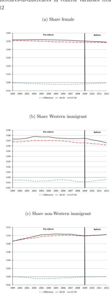
Figure A.3: Differences-in-differences in control variables treatment and control group: 1999–2012
(a) Share female
-0.10 0.00 0.10 0.20 0.30 0.40 0.50 0.60
1999 2000 2001 2002 2003 2004 2005 2006 2007 2008 2009 2010 2011 2012
Difference 20-25 27-29
Pre-reform Reform
Pre-reform Reform
(b) Share Western immigrant
-0.02 -0.01 0.00 0.01 0.02 0.03 0.04 0.05 0.06 0.07 0.08 0.09
1999 2000 2001 2002 2003 2004 2005 2006 2007 2008 2009 2010 2011 2012
Difference 20-25 27-29
Pre-reform Reform
Pre-reform Reform
(c) Share non-Western immigrant
-0.02 0.00 0.02 0.04 0.06 0.08 0.10 0.12
1999 2000 2001 2002 2003 2004 2005 2006 2007 2008 2009 2010 2011 2012
Difference 20-25 27-29
Pre-reform Reform
Pre-reform Reform
Source: Own calculations using the Labour Market Panel (Statistics Netherlands). The solid black lines denote the control group (27–28 years of age), the dashed red lines denote the treatment group (25–26 years of age) and the
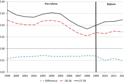
Figure A.4: Differences-in-differences in outcome variables of individuals aged 20-26 and 27-29: 1999–2012
(a) NEETs rate on welfare
-0.02 -0.01 0.00 0.01 0.02 0.03 0.04
1999 2000 2001 2002 2003 2004 2005 2006 2007 2008 2009 2010 2011 2012 Difference 20-26 27-29
Pre-reform Reform Pre-reform Reform
(b) NEETs rate not on welfare
-0.06 -0.04 -0.02 0.00 0.02 0.04 0.06 0.08 0.10 0.12
1999 2000 2001 2002 2003 2004 2005 2006 2007 2008 2009 2010 2011 2012 Difference 20-26 27-29
Pre-reform Reform Pre-reform Reform
(c) Total NEETs rate
-0.08 -0.06 -0.04 -0.02 0.00 0.02 0.04 0.06 0.08 0.10 0.12 0.14 0.16
1999 2000 2001 2002 2003 2004 2005 2006 2007 2008 2009 2010 2011 2012 Difference 20-26 27-29
Pre-reform Reform Pre-reform Reform
(d) Employment rate
-0.40 -0.20 0.00 0.20 0.40 0.60 0.80 1.00
1999 2000 2001 2002 2003 2004 2005 2006 2007 2008 2009 2010 2011 2012 Difference 20-26 27-29
Pre-reform Reform Pre-reform Reform
(e) Enrollment rate in education
0.00 0.05 0.10 0.15 0.20 0.25 0.30 0.35
1999 2000 2001 2002 2003 2004 2005 2006 2007 2008 2009 2010 2011 2012 Difference 20-26 27-29
Pre-reform Reform Pre-reform Reform
Notes: Own calculations using the Labour Market Panel (Statistics Netherlands). The solid black lines denote the control group (27–29 years of age), the dashed red lines denote the treatment group (20–25 years of age) and
the dotted blue lines denote the difference between the treatment group and the control group. NEETs rates
are individuals not in employment or in education relative to the relevant age population, employment rates are
individuals in employment relative to the relevant age population and enrollment rates are individuals in education
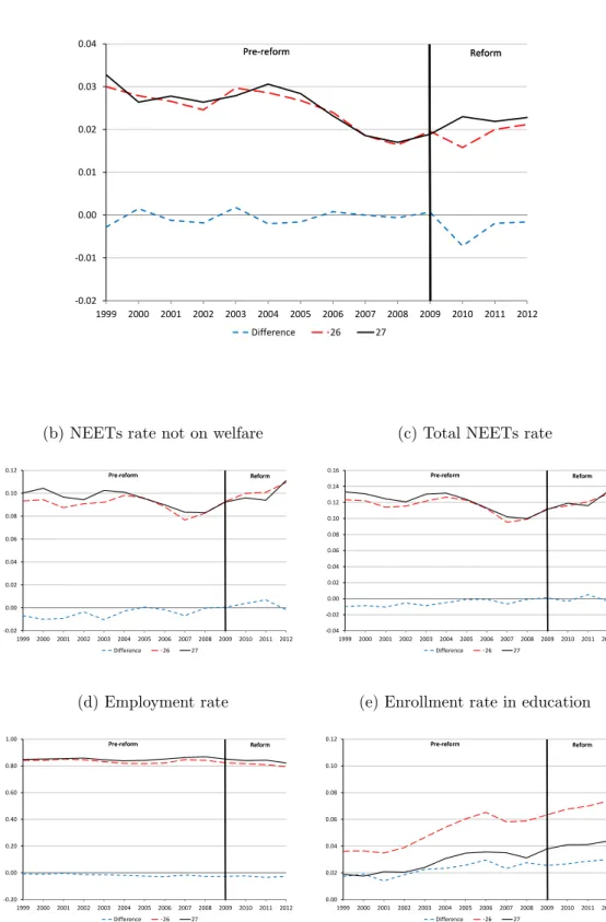
Figure A.5: Differences-in-differences in outcome variables of individuals aged 26 and 27: 1999–2012
(a) NEETs rate on welfare
-0.02 -0.01 0.00 0.01 0.02 0.03 0.04
1999 2000 2001 2002 2003 2004 2005 2006 2007 2008 2009 2010 2011 2012
Difference 26 27
Pre-reform Reform Pre-reform Reform
(b) NEETs rate not on welfare
-0.02 0.00 0.02 0.04 0.06 0.08 0.10 0.12
1999 2000 2001 2002 2003 2004 2005 2006 2007 2008 2009 2010 2011 2012 Difference 26 27
Pre-reform Reform Pre-reform Reform
(c) Total NEETs rate
-0.04 -0.02 0.00 0.02 0.04 0.06 0.08 0.10 0.12 0.14 0.16
1999 2000 2001 2002 2003 2004 2005 2006 2007 2008 2009 2010 2011 2012 Difference 26 27
Pre-reform Reform Pre-reform Reform
(d) Employment rate
-0.20 0.00 0.20 0.40 0.60 0.80 1.00
1999 2000 2001 2002 2003 2004 2005 2006 2007 2008 2009 2010 2011 2012 Difference 26 27
Pre-reform Reform Pre-reform Reform
(e) Enrollment rate in education
0.00 0.02 0.04 0.06 0.08 0.10 0.12
1999 2000 2001 2002 2003 2004 2005 2006 2007 2008 2009 2010 2011 2012 Difference 26 27
Pre-reform Reform Pre-reform Reform
Notes: Own calculations using the Labour Market Panel (Statistics Netherlands). The solid black lines denote the control group (27–29 years of age), the dashed red lines denote the treatment group (20–25 years of age) and
the dotted blue lines denote the difference between the treatment group and the control group. NEETs rates
are individuals not in employment or in education relative to the relevant age population, employment rates are
individuals in employment relative to the relevant age population and enrollment rates are individuals in education
34
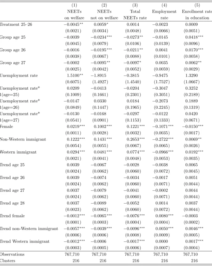
Table A.1: Differences-in-differences: full results base regressions
(1) (2) (3) (4) (5)
NEETs NEETs Total Employment Enrollment rate
on welfare not on welfare NEETs rate rate in education
Treatment 25–26 −0.0045∗∗ 0.0059∗ 0.0014 −0.0023 0.0009
(0.0021) (0.0034) (0.0048) (0.0066) (0.0051)
Group age 25 −0.0039 −0.0234∗∗∗ −0.0273∗∗ −0.0145 0.0418∗∗∗
(0.0045) (0.0079) (0.0106) (0.0139) (0.0096)
Group age 26 −0.0016 −0.0195∗∗∗ −0.0211∗∗ 0.0041 0.0170∗∗∗
(0.0038) (0.0067) (0.0088) (0.0101) (0.0058)
Group age 27 −0.0002 −0.0095∗∗ −0.0097∗ 0.0035 0.0062∗∗
(0.0025) (0.0042) (0.0052) (0.0059) (0.0029)
Unemployment rate 1.5100∗∗ −1.8915 −0.3815 −0.9475 1.3290
(0.6075) (1.4927) (1.4540) (1.7527) (1.0667)
Unemployment rate* 0.0209 −0.0413 −0.0204 −0.3047 0.3252
1(age=25) (0.1009) (0.1661) (0.2301) (0.3051) (0.2189)
Unemployment rate* −0.0147 0.0330 0.0184 −0.2073 0.1889
1(age=26) (0.0849) (0.1447) (0.1965) (0.2245) (0.1319)
Unemployment rate* −0.0130 −0.0168 −0.0297 −0.0122 0.0420
1(age=27) (0.0541) (0.0901) (0.1153) (0.1333) (0.0671)
Female 0.0219∗∗∗ 0.1002∗∗∗ 0.1221∗∗∗ −0.1071∗∗∗ −0.0150∗∗∗
(0.0011) (0.0028) (0.0032) (0.0035) (0.0017)
Non-Western immigrant 0.1222∗∗∗ 0.1431∗∗∗ 0.2653∗∗∗ −0.2722∗∗∗ 0.0069∗∗
(0.0054) (0.0055) (0.0067) (0.0065) (0.0026)
Western immigrant 0.0294∗∗∗ 0.0481∗∗∗ 0.0774∗∗∗ −0.0966∗∗∗ 0.0192∗∗∗
(0.0021) (0.0041) (0.0048) (0.0053) (0.0035)
Trend age 25 0.0039 −0.0067 −0.0028 −0.0038 0.0065
(0.0024) (0.0062) (0.0060) (0.0072) (0.0045)
Trend age 26 0.0039 −0.0074 −0.0034 −0.0017 0.0051
(0.0024) (0.0062) (0.0060) (0.0071) (0.0044)
Trend age 27 0.0037 −0.0079 −0.0041 −0.0002 0.0044
(0.0024) (0.0062) (0.0060) (0.0071) (0.0044)
Trend age 28 0.0037 −0.0089 −0.0052 0.0014 0.0037
(0.0023) (0.0062) (0.0060) (0.0072) (0.0044)
Trend female −0.0012∗∗∗ −0.0065∗∗∗ −0.0076∗∗∗ 0.0080∗∗∗ −0.0003
(0.0001) (0.0003) (0.0004) (0.0004) (0.0002)
Trend non-Western immigrant −0.0057∗∗∗ −0.0039∗∗∗ −0.0096∗∗∗ 0.0050∗∗∗ 0.0046∗∗∗
(0.0006) (0.0006) (0.0008) (0.0009) (0.0005)
Trend Western immigrant −0.0012∗∗∗ −0.0006 −0.0017∗∗∗ 0.0000 0.0017∗∗∗
(0.0003) (0.0005) (0.0006) (0.0007) (0.0004)
Observations 767,710 767,710 767,710 767,710 767,710
Clusters 216 216 216 216 216
Notes: * denotes significant at the 10% level, ** at the 5% level and *** at the 1% level. Sample period 1999–2012. Treatment group 25–26 and control group 27–28. Cluster-robust standard errors in parentheses, clustered by year of birth*province (18*12=216). Year