Stepwise Variable Selection for Loglinear Mixture in Record Linkage

EUROPEAN JOURNAL OF PURE AND APPLIED MATHEMATICS Vol. 3, No. 2, 2010, 141-162

ISSN 1307-5543 – www.ejpam.com

Stepwise Variable Selection for Loglinear Mixtures in Record

Linkage

Rong Zhu

_{, Jin Zhang}

_{, Da Zhang}

_{, Guohua Yan}

1_{Department of Mathematics and Statistics, McMaster University, Canada} 2_{Office of Institutional Research and Analysis, McMaster University, Canada} 3_{Department of Computer Science Technology, Ohio University Lancaster, USA} 4_{Department of Mathematics and Statistics, University of New Brunswick, Canada}

Abstract. A model building strategy is proposed to improve the probabilistic match in record linkage with focus on the loglinear mixture model of two components, each for the matched and unmatched pairs respectively. In reality, comparison attributes (i.e., covariates) often interact with each other, leading to more or less interactions in the loglinear models for both the matched and unmatched pairs. However, the interactions patterns are often not the same for both components. Particularly, because the number of matched pairs is usually very small compared with that of unmatched pairs in prac-tice, the model for matched pairs can not be fitted with the same higher order interactions as that for the unmatched pairs. The proposed strategy is data-driven, and attempts to avoid both underfitting and overfitting due to subjective model specification for the data. Starting from the situation of no interaction, we add interactions sequentially in two loglinear components using the forward selection approach. Specifically, we define the alternatively climbing pathways through mixture families of two components with higher order interactions. The mixture models expanded along a pathway are nested successively. Thus, conventional tests used for comparison of nested models can be applied. Regard-ing parameter estimation for the mixture, a simplified method (includRegard-ing the choice of initial values of parameters) for the EM algorithm is developed, which facilitates the mixture model fitting using existing packages and functions in sophisticated statistical software like R. Simulation studies have then been conducted for various situations to assess the model selection approach, and comparisons of the selected models with the naive model assuming field independence have been made. We have applied this strategy to the record linkage case study in 2006 Annual Meeting of Statistical Society of Canada (SSC) and identified interactions among certain comparison attributes for both matched and unmatched pairs; these interactions are not always the same for both mixture components.

2000 Mathematics Subject Classifications: 62F07, 62F10, 62J99, 62P25

Key Words and Phrases: record linkage, loglinear mixture models, EM algorithm, model selection, alternatively climbing pathways

∗_{Corresponding author.}

Email addresses: rzhumath.mmaster.a(R. Zhu),zhangjnmmaster.a(J. Zhang),

zhangd1ohio.edu(D. Zhang),gyanunb.a(G. Yan)

1. Introduction

Information often comes from various sources regarding different aspects of objects, and could be recorded at different time points. For example, the provincial resident registry infor-mation is comprised of several data sources from different departments such as transportation, health, license and registration. These data sets include specific personal information such as name, date of birth and address. Typically, there is no unique ID assigned to individual ob-jects among all data sources. However, for some reasons, like administration or detection of particular interested individuals (say, terrorists), the need arises to link two or more data sources together so that the records for the same individual object across different files can be identified for further processing. This task also identifies duplicate records in one file where a second virtual file is the copy of the original one.

The way to decide whether two records are the same or whether two records describe the same object is called record linkage. Records in different data files consist of common attributes (such as name, address and date of birth) and different attributes (such as weight in one file and height in another file) for individual objects. Usually, the common attributes are chosen to be identifiers for record matching. However, the different attributes in two files may provide partial information for the matching if these attributes are highly associated. In this study, we only consider the common attributes as the identifiers. Comparison vectors are then obtained for each record pair by comparing the values of identifiers.

The status of a pair of records for comparison is either “matched” or “unmatched”. Ideally, if the values of identifiers match exactly for a record pair, then the two records are from the same object. However, in reality, there are many situations where the values of identifiers may not be the same even if they are from the same object. For example, the surname of a female may change when her marriage status changes. Hence, the method of exact match or deterministic match may miss many matched records. On the other hand, exact match may not always imply the same object. For instance, if the identifiers are just name and date of birth, it could occur that two different persons have the same name and date of birth although the chance is small. For this reason, probabilistic match is employed where the pair of records is regarded as from the same object if the weight involving the matched and unmatched probabilities is large enough.

Historically, Newcombe et al. (1959) studied probabilistic linkage on vital records; refer to[13]. Fellegi and Sunter (1969) developed the formal mathematical framework for prob-abilistic record linkage, and they also specified models in a hierarchical way according to a possible error-making mechanism; see [6]. After that, many techniques and software have been developed for record linkage. For example, blocking is used to reduce not only the size of comparison pairs, but also the dependence effects (i.e., interaction between identifiers). Nowadays record linkage methodology is used in many areas such as census, survey, admin-istration and medical research; see[1, 3, 8, 12].

R. Zhu, J. Zhang, D. Zhang, G. Yan Eur. J. Pure Appl. Math,3(2010), 141-162 143

and used the EM algorithm for parameter estimation with application in a test census of Tampa in 1985; see [7]. Winkler (1989) presented a loglinear model to adjust the lack of independence; refer to[16]. More work on loglinear models can be found in[8, 9, 10], and references therein.

We focus on mixture models. For a given record linkage task, many mixture models can be specified. However, which model fits the observed comparison pairs better, and how can underfitting or overfitting be avoided? These are questions for record linkage practitioners. Our study is motivated by the record linkage case study in 2006 Annual Meeting of Statistical Society of Canada (SSC 2006). We tried some free software for record linkage and found that their models assume field independence without interactions. The possible reason for this limitation could be the computational burden for arbitrary mixture models. However, the lack of fit is obvious in this simple model if fields are dependent. On the other hand, subjectively specifying models with higher order interactions may lead to overfitting for one or both components. Both underfitting and overfitting will affect the calculation of matched and unmatched probabilities, and thus affect the partition of record pairs. These problems lead to the model selection in the mixture setting.

In our study, we propose a strategy for model selection in loglinear mixtures, where pa-rameter estimates are obtained via a simplified method for the EM algorithm for the mixture of two components. Such a simplified method can take advantage of existing packages and functions in sophisticated statistical software like R, so computationally it is tractable. We define the alternatively climbing pathways to indicate a sequence of nested models in the mixture family. For comparison, we adopt the Pearson Chi-square test for nested models on alternatively climbing pathways. The feature of this strategy is data-driven, and thus, the model building avoids subjective specification. Simulation studies have been conducted to verify the strategy, and to acquire experience of model building. We compare the results from this strategy with those from the simplest model where all factors are binary and independent. It shows that the data-driven strategy does give a refinement on modelling and lead to more accurate estimation of probabilities compared with the simplest model.

This paper is organized as follows. We outline statistical modelling and a simplified method for the EM algorithm in record linkage in Section 2. In Section 3, we propose the data-driven strategy for modelling loglinear mixtures. Then we conduct simulation studies to assess the proposed strategy in Section 4, and apply it to a case study in Section 5. Finally, we make brief concluding remarks in Section 6.

2. Statistical framework and parameter estimation for record linkage

2.1. Notation and framework

Consider two files where fileAhas arecords and file B has brecords. The total number of possible record pairs for comparison isN =a×b. The records consist of attributes which can be categorical variables such as name, address and date of birth, or numerical variables such as age. Selectncommon attributes as the identifiers for comparing pairs of records from both files A and B. Then the comparison for each record pair is made for all n identifiers by matching rules defined according to the needs for these attributes. This will result in a comparison vector of length n with each component being categorical. Each component associated with an identifier (attribute) in the comparison vector is called a field. The field values of comparison vector could be binary like 0 and 1, or any others defined by some rules. For example, the simplest rule is agreement/disagreement on an attribute. Under this simplest rule, if comparison attributes are name, address, gender and date of birth, an observed comparison vector (0, 1, 1, 0)means disagreement on name and date of birth, but agreement on address and gender. Thus, we obtainN comparison vectors for all record pairs denoted as follows:

γj = (γ₁j, . . . ,γ_nj), j=1, . . . ,N,

where the subscript denotes the comparison field while the superscript indicates the compar-ison pair.

Note that all comparison pairs include two types of pairs: matched and unmatched. There-fore, we can view the entire population of all possible comparison pairs as a mixture of two components or subpopulations: matched pairs and unmatched pairs. However, in this mix-ture, the membership for each pair is missing or unknown.

Let M denote the matched subpopulation and U denote the unmatched subpopulation. Each pair is either fromM orU. Let

m_j=P(γj|M), u_j=P(γj|U), j=1, . . . ,N.

Define the matching weight as follows:

w_j=logP(γ

j_|M)

P(γj_|U) =logP(γ

j_{|M)−logP(γ}j_{|U), j=1, . . . ,N,}

the logarithm of the likelihood ratio between the matched and unmatched. Probabilistic mod-els are specified to obtain the associated probabilities.

Fellegi and Sunter (1969) set the fundamental probabilistic framework for record linkage; see [6]. Assume that mj,uj,wj are estimated from data. Without loss of generality, the

descending matching weight sequence is assumed to be

w1≥. . .≥wk≥. . .≥wl≥. . .≥wN,

and the corresponding matched and unmatched probability sequences are

R. Zhu, J. Zhang, D. Zhang, G. Yan Eur. J. Pure Appl. Math,3(2010), 141-162 145

u₁, . . . ,u_k,| . . . , |u_l, . . . ,u_N,

where k and l are the cutting points which partition all comparison pairs into three parts: matched, uncertain and unmatched, as follows:

C₁: j=1, . . . ,k; matched,

C₂: j=k+1, . . . ,l−1; uncertain for clerical review,

C3: j=l, . . . ,N; unmatched.

The cutting conditions are set as

k X

j=1

u_j≤α1, N X

j=l

m_j≤α2, whereα1andα2are prespecified.

A good tutorial was given by Fair and Whitridge (1997); see[5]. In addition, Winkler (2005) gave an overview on record linkage; refer to[17].

In the literature, various models have been proposed for the mixture population from dif-ferent angles. We have mentioned a few in Section 1. In this study, we focus on loglinear mixture models. The advantage of using a parametric model is that we can ignore the un-derlying error-making mechanism. Note that the mixture models for record linkage consist of only two components. In next subsection, we will outline the general framework for this particular type of mixture models and propose a simplified method for the EM algorithm as well as the choice of initial parameter values for this method.

2.2. Mixture models and the simplified method of the EM algorithm for

parame-ter estimation

We consider parametric models for both the matched and unmatched subpopulations. Assume that the model forM has pmf or pdf f_M(γ;β_m)while the model forU has pmf or pdf

fU(γ;βu). Hereγis the comparison vector, andβm andβu are parameter vectors associated

with the models for M andU respectively. Suppose the chance of a comparison pair fromM

isπ. Then the pmf or pdf for the j-th comparison pair is

f_γ(γj;β_m,β_u,π) =πf_M(γj;β_m) + (1−π)f_U(γj;β_u). (1)

On the other hand, denote the membership for the j-th comparison pair as follows

g_j= (

1, ifγj is from the matched populationM,

0, ifγj is from the unmatchedU, j=1, . . . ,N.

For the j-th pair, the complete data is Xj = (γj,gj). Thus, the pmf or pdf for the complete

data of the j-th pair is

Assume that the comparison pairs are independent. The logarithm of the joint pmf or pdf for all complete data is

l_C€(γ1,g₁), . . . ,(γN,g_N);β_m,β_u,πŠ=log



 

N Y

j=1

f_X€(γj,g_j);β_m,β_u,πŠ    = N X

j=1 ”

g_jlogf_M(γj;β_m) + (1−g_j)logf_U(γj;β_u)

+gjlogπ+ (1−gj)log(1−π) —

. (3)

The conditional pmf for the membershipgis then

f_g|γ€g_j|γj;β_m,β_u,πŠ = fX €

(γj,gj);βm,βu,π Š

f_γ(γj_;β

m,βu,π)

= fX

€ (γj_,g

j);βm,βu,π Š

πfM(γj;βm) + (1−π)fU(γj;βu)

. (4)

However, the membership g_j is missing in the mixture population. Therefore, the mixture can be regarded as a missing value problem and the EM algorithm can be utilized to estimate the model parametersβ_m,β_u andπ. For references on the EM algorithm, see[4],[11]and references therein.

The EM algorithm is an iterative approach which alternates between two steps, an E-step and an M-step. The E-step is conducted as follows. Conditional on values ofβ(_mk), β(_uk)and

π(k)_{, as well as the observed comparison vectors, the expectation of the logarithm of the joint} pmf or pdf for all complete data is

L = E”l_C€(γ1,g₁), . . . ,(γN,g_N);β_m,β_u,πŠ|γ1, . . . ,γN;β_m(k),β(_uk),π(k)— =

N X

j=1

E”log€f_X€(γj,g_j);β_m,β_u,πŠŠ|γj;β(_mk),β(_uk),π(k)—

= N X

j=1 Z

log”f_X€(γj,g_j);β_m,β_u,πŠ—f_g|γ€g_j|γj;β(_mk),β_u(k),π(k)Šd g_j

= N X

j=1 1 X

gj=0

¦”

gjlogfM(γj;βm) + (1−gj)logfU(γj;βu)

+gjlogπ+ (1−gj)log(1−π) —

×fg|γ €

gj|γj;β(mk),β (k) u ,π

(k)Š©

.

Let

g_m(k)(γj) = f_g|γ€1|γj;β(_mk),β_u(k),π(k)Š= π (k)_f

M(γj;β(mk))

π(k)_f

M(γj;β(mk)) + (1−π(k))fU(γj;β(uk))

R. Zhu, J. Zhang, D. Zhang, G. Yan Eur. J. Pure Appl. Math,3(2010), 141-162 147

g_u(k)(γj) = fg|γ €

0|γj;β(_mk),β_u(k),π(k)Š= (1−π (k)_)f

U(γj;β(uk))

π(k)_f

M(γj;β(mk)) + (1−π(k))fU(γj;β(uk)) = 1−g_m(γj).

Then, by algebra,

L = N X

j=1

g_m(k)(γj)logfM(γj;βm) + N X

j=1

g_u(k)(γj)logfU(γj;βu)

+ N X

j=1 ”

g_m(k)(γj)logπ+g_u(k)(γj)log(1−π)—

= L₁+L₂+L₃,

where

L1= N X

j=1

g_m(k)(γj)logfM(γj;βm), L2= N X

j=1

g_u(k)(γj)logfU(γj;βu),

and

L₃= N X

j=1 ”

g_m(k)(γj)logπ+g_u(k)(γj)log(1−π)—.

This splits the conditional expectationLinto three separate parts corresponding to the matched pairs, the unmatched pairs and the mixing proportionπrespectively.

The M-step maximizes the conditional expectation L, which is in turn equivalent to maxi-mization ofL₁, L₂and L₃separately. Note that L₁andL₂ are weighted log-likelihoods for the matched and unmatched pairs respectively. Thus, for models which can be fitted by weighted MLE using available software, their maximization can be readily obtained by that software. The maximization ofL₃is straightforward:

∂L3 ∂ π =

N X

j=1

g(_mk)(γj)1 π−g

(k) u (γ

j₎ 1

1−π =0 yields 1 π N X

j=1

g_m(k)(γj) = 1 1−π

N X

j=1

g_u(k)(γj).

Thus,

π=

PN j=1g

(k) m (γj) PN

j=1g (k) m (γj) +

PN j=1g

(k) u (γj)

= 1

N

N X

j=1

We obtain

π(k+1)= 1

N

N X

j=1

g_m(k)(γj), β(_mk+1)=arg maxL₁, β(_uk+1)=arg maxL₂. (5)

This approach is regarded as a simplified method of the EM algorithm for the mixture situ-ation. It can take advantage of existing packages or functions in statistical software without developing particular code for maximization of the complicated model components, especially with interactions. Note that Winkler (1988) investigated the EM algorithm for Fellegi-Sunter model; see[15]. We are suggestting a computational method for fitting a mixture with two components where each component is readily fitted by a model like GLM.

3. Model building strategy for loglinear mixtures of two components

We consider all fields of the comparison vectorγ= (γ1, . . . ,γn)are categorical. For

exam-ple,γ1 could be binary taking value 0 or 1, meaning unmatching or matching respectively for

a pair of records in field 1. Then all of such observed comparison vectors form a multi-way contingency table with nfactors (each field corresponds to a factor). Thus, it is natural to utilize the loglinear model for analyzing such a contingency table.

A loglinear model states that the logarithm of the expected number of a cell in the con-tingency table can be expressed as the additive function of main effects and interactions of factors. For instance, we consider a four factorI×J×K×Lcontingency table. Two loglinear models we will use in the remaining are

logµi jkl=λ+λ (1)

i +λ

(2)

j +λ

(3)

k +λ

(4)

l , (6)

or

logµi jkl=λ+λ (1)

i +λ

(2)

j +λ

(3)

k +λ

(4)

l +λ

(12) i j +λ

(13)

ik +λ

(14)

il +λ

(23)

jk +λ

(24)

jl +λ

(34)

kl , (7)

i=1, . . . ,I; j=1, . . . ,J; k=1, . . . ,K, l=1, . . . ,L.

Here µi jkl denotes the expected cell count, λ is the overall mean, λ (1) i , λ

(2) j , λ

(3)

k and λ

(4) l

are the main effects of each factor at corresponding levels i,j,k and l, λ(_{i j}12), λ(_ik13), λ(_il14),

λ(_jk23),λ(_jl24),λ(_kl34)are two-factor interactions at specified level pairs. Model (6) corresponds to the situation of independence among factors, while model (7) corresponds to a situation of dependence among factors. Note that model (6) is nested in model (7).

Apart from the above common ANOVA-like formulation, there is a generalized linear model formulation, where the cell counts are assumed to be distributed in Poisson. For in-stance, Model (6) and (7) have the following equivalent Poisson GLM formulations:

logµ=α+α1γ1+α2γ2+α3γ3+α4γ4, (8)

and

R. Zhu, J. Zhang, D. Zhang, G. Yan Eur. J. Pure Appl. Math,3(2010), 141-162 149

+α12γ1γ2+α13γ1γ3+α14γ1γ4+α23γ2γ3+α24γ2γ4+α34γ3γ4. (9)

Hereα’s are the intercept for the model and coefficients for variableγ’s and their interactions,

µis the expected cell count associated with covariatesγ= (γ1,γ2,γ3,γ4).

R has functionloglm()for fitting loglinear models in the form of ANOVA-like specifica-tion, and functionglm()for fitting Poisson GLM models. Each has advantages and disadvan-tages. We use both in our computation in case one encounters unexpected problems.

In record linkage, the matched and unmatched subpopulations could have their own model specifications, thus, M andU are assumed to have different loglinear models respec-tively. However, the membership is unknown. So the entire population of possible pairs is a mixture of two loglinear models for M andU. The observed contingency table is a sample from this mixture population.

Jaro (1989) considered the simplest case for the contingency table where all factors are binary, and thus, the contingency table is 2×2× · · · ×2, and the number of all cells of the table is 2n; see[7]. He assumed field independence, and employed the EM algorithm for the estimation of all probabilities related to fields and the mixing proportion. From the prospec-tive of loglinear model formulation, the models for M and U in Jaro (1989) were loglinear models without interactions. The field independence may not hold in reality. For instance, strong dependencies were observed by Thibaudeau (1993) in census data; see[14]. Prior to that report, Winkler (1989) extended the simplest case to a general one, where interactions were taken into account in the models forM andU, specifically, two-class and three-class in-teractions were considered, and models were assessed using goodness-of-fit tests (see[16]). Larsen (1997) considered a loglinear model with main effects, all two-way interactions, all three-way interactions and two five-way interactions in a trial census and post-enumeration survey (see[9]).

Any of the specified loglinear mixture models can be estimated using the simplified method for the EM algorithm in Section 2. For a real case, the specification can be given from back-ground information or subjective opinion. Thus, different opinions or understanding about the real case can result in different model specifications.

However, among those subjectively specified models, which one fits the observed con-tingency table better, or captures the data feature better? How can we avoid overfitting or underfitting? These questions lead to the model selection for loglinear mixture models in record linkage. Usually, a better model will give a better estimation of cell probabilities for matched and unmatched pairs, which in turn increases the accuracy of record pair partition.

When we search among a series of models, a method of statistical testing is required for model comparison at each step, and a strategy is needed in the iterative selection process. Suppose the loglinear mixture modelM(0)is nested in another loglinear mixture modelM(1), namelyM(0) ⊂ M(1). We adopt a general method to compare these two loglinear mixture models, i.e., testing

H₀: M(0)=M(1) versus H₁: M(0)⊂ M(1).

employed as follows

χ2€M(0)_|M(1)Š

=X( ˆµ_1i−µˆ_0i)2/µˆ_0i, (10)

whereµˆ1i andµˆ0i are fitted values of individual cell expectations forM(0)andM(1)

respec-tively. Because one model is nested in the other, the asymptotic distribution ofχ2€M(0)|M(1)Š

underH0isχ2(d f), where the degrees of freedomd f is the difference of parameter numbers

betweenM(0)andM(1). For a reference, see[2], P. 364.

The loglinear models for components U and M in the mixture we consider for record linkage may or may not include higher order interactions among fields. We denoteMi j for a

loglinear mixture model whereiindicates that the loglinear model forU has up to the (i+ 1)-th order interactions (i.e., (i+1)-factor-interactions) and j indicates that the loglinear model forM has up to the (j+1)-th order interactions (i.e., (j+1)-factor-interactions), i,j ≥0. For instance,M₀₀means that the models for both M andU in the mixture have no interactions, i.e., Model (6).M₁₀means that the model forU has two-factor interactions, while the model for M has no interactions. M02 means that the model for U has no interactions, while the

model forM has two-factor and three-factor interactions. The nested situation of two loglin-ear mixture models is totally determined by the nested situations of their both components. Therefore, we can build nested loglinear mixture models by building nested loglinear models for eitherU orM, or bothU andM. That is,

Mi j⊂ Mi′j′ ifi≤i′and j≤ j′.

For instance,M₀₀⊂ M₀₁⊂ M₁₁andM₀₀⊂ M₁₀⊂ M₁₁, butM₀₁andM₁₀are not nested in each other. See the illustration in (11) where mixture models of two components are arranged in a matrix format.

..

. ... ... ...

M30 M31 M32 → M33 · · ·

↑ ⇑

M20 M21 → M22 ⇒ M23 · · ·

↑ ⇑

M₁₀ → M₁₁ ⇒ M₁₂ M₁₃ · · ·

↑ ⇑

M00 ⇒ M01 M02 M03 · · ·

(11)

We make comparison for models on the nested pathways. However, there are many nested paths in the family of loglinear mixtures of two components. For example, fromM00toM11,

there are two nested pathways: M₀₀ ⊂ M₁₀ ⊂ M₁₁ and M₀₀⊂ M₀₁ ⊂ M₁₁. In general, from one diagonal modelM_ii to the next diagonal modelM_(i+1)(i+1), there are two nested pathways similar to this illustrated example. Refer to (11). This pair of nested pathways is called alternatively climbing pathways (denoted by “→” and “⇒” respectively). We propose the following forward selection strategy along the alternatively climbing pathways:

R. Zhu, J. Zhang, D. Zhang, G. Yan Eur. J. Pure Appl. Math,3(2010), 141-162 151

• Step 2: Proceed on the pathwayM00⊂ M10⊂ M11, and compare two adjacent models

successively using a prespecified significance levelα. This pathway considers the model with higher order interactions forU first.

– If the series testing stops atM₀₀, then go to step 3.

– If the series testing stops atM10, then the final model isM10.

– If the series testing stops atM₁₁, then go to step 4.

• Step 3: Proceed on the alternative pathway M00 ⊂ M01 ⊂ M11, and compare two

adjacent models successively using the significance levelα. This pathway considers the model with higher order interactions forM first.

– If the series testing stops atM₀₀, then the final model isM₀₀. – If the series testing stops atM01, then the final model isM01.

– If the series testing stops atM11, then go to step 4.

• Step 4: TreatM11 like M00, and repeat steps 1 to 3 along the alternatively climbing

pathways fromM11toM22, i.e., start a second round of search from the next diagonal

entry.

• Step 5: Continue the iteration until the series testing stops.

The above search on alternatively climbing pathways guarantees the nesting between two loglinear mixture models under comparison. We place priority on the pathway where the model for U is added higher order interactions (the route denoted by “→”) first, because in record linkage, the unmatched pairs are the majority. If this fails, then we consider the other pathway where the model for M is added higher order interactions (the route denoted by “⇒”).

Note that for step 1, if the contingency table degenerates to the case where all factors are binary, the computation will become the Jaro’s method. The simplest loglinear mixture model M00captures the main effects explained by factors alone. Note that the attributes chosen by

investigators are typically important variables in record matching according to background knowledge. Thus, their main effects practically exist. On the other hand, we may not know the joint effects of attributes in advance. Thus, it is safe and convenient to start from the simplest mixture modelM00.

However, if the joint effects have been known to be strong by the background knowledge, we can start from a particular mixture model which may not be a diagonal entry in (11). A modification of the model search is then that we proceed with the testings on an upward or a rightward pathway to the model in the closest diagonal entry, then continue the search using the above strategy. Note that the backward selection could be feasible. However, it starts from the most complicated model with all possible interactions, and thus, the computational cost is typically large.

In record linkage, the number of matched pairs is extremely small relative to the number of unmatched pairs. So usually the model for M has lower order interactions than that for

along the alternatively climbing pathways prevents over-extension of model for either compo-nentU or M. This conservative procedure is based on the reasoning that interactions among attributes usually affect both subpopulationsU and M. Thus, we do not wish the model for

U has higher order interactions while the model for M does not. If this reasoning is not ap-propriate, the restriction can be relaxed, say we can further extend the model forU when a final model isM_(i+1)i. However, our simulation studies show that it is hard to capture higher order interactions from data even if they are truly generated from a model with higher order interactions. Therefore, from the practical viewpoint, we suggest not to seek very higher order interactions in record linkage.

The final model obtained from the proposed strategy will include all interactions of the same order, say all three-factor-interactions or third order interactions. It may not be neces-sary to do so because some of them could be very weak. Thus, we can apply testing in (10) again to prune unnecessary interactions for eitherU or M in the final mixture model.

The choice of initial values of parameters for the EM algorithm is important for the final solution. If the contingency table is the one with binary factors, then we can use the Jaro’s method to determine the initial values. Note that the maximum number of matched pairs is min(a,b). In a general case, we propose the following data-driven method named as the J method for the choice of initial values regarding parametersπ,β_uandβ_m:

• the initial value for the mixing proportion is chosen asπ(0)=min(a,b)/a b=1/max(a,b), the upper bound of the mixing proportion. This can be modified asπ(0)/10,π(0)/5 or

π(0)_{/2 depending on the blocking situation.}

• β(_u0), the vector of initial values in the loglinear model for U, is obtained from fitting that model to a modified table which has more unmatched pairs and fewer matched pairs. The cell values of this table are the original cell counts divided by min(a,b)(thus may not be integers).

• β(_m0), the vector of initial values in the loglinear model for M, is obtained from fitting that model to another modified table which is created by picking counts for cells with higher matching chance, and assigning zeroes for others cells.

Intuitively, if the table is derived from more unmatched pairs or from more matched pairs, then the fitted model is closer to the true model for U or for M respectively. It works quite well in the simulation studies. Note that fitting a loglinear model to a non-integer-valued table is the same as fitting to an integer-valued table in R.

4. Simulation Studies

Simulation studies are necessary for verifying the proposed data-driven strategy of model building. From simulation, we can obtain experience on model fitting and building in various settings such as file sizes, mixing proportions and interactions patterns. Besides, we can also identify potential drawbacks for necessary adjustment.

We consider the comparison vector consisting of four fields, γ= (γ1,γ2,γ3,γ4), which is

R. Zhu, J. Zhang, D. Zhang, G. Yan Eur. J. Pure Appl. Math,3(2010), 141-162 153

indicates the field matched. Thus, the total number of cells is 24 =16. Table 1 labels all of these sixteen cells in the way of a 24 factorial design matrix for later reference. Commonly,

Table1: Celllabelsforthe2×2×2×2ontingenytable.

Cell Comparison vector Cell Comparison vector

1 (0, 0, 0, 0) 9 (0, 0, 0, 1)

2 (1, 0, 0, 0) 10 (1, 0, 0, 1) 3 (0, 1, 0, 0) 11 (0, 1, 0, 1) 4 (1, 1, 0, 0) 12 (1, 1, 0, 1) 5 (0, 0, 1, 0) 13 (0, 0, 1, 1) 6 (1, 0, 1, 0) 14 (1, 0, 1, 1) 7 (0, 1, 1, 0) 15 (0, 1, 1, 1) 8 (1, 1, 1, 0) 16 (1, 1, 1, 1)

a cell with more 1’s has larger matching chance for record pairs with comparison vectors in that cell. Thus, cells corresponding to comparison vectors being (1, 1, 1, 1),(1, 1, 0, 1) and (1, 1, 1, 0)have more matching possibilities than cells corresponding to(0, 0, 0, 0),(0, 0, 1, 0) and(0, 0, 0, 1).

This is the type of contingency table considered in Jaro (1989); see [7]. For this situa-tion, a byproduct is that we can compare the estimated 16 cell probabilities from the model selected via the data-driven strategy with those from the simplest starting model M00. For

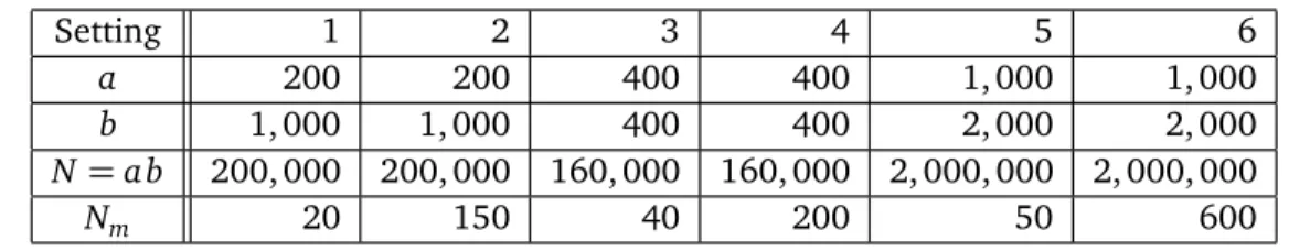
each individual simulation, we set the lengths of two data sets asaand b, as well as the true matched pairs N_m (thus, leading to the mixing proportion π). For the sake of simplicity, we do not consider the blocking technique, thus, there areN =a brecord pairs. Six settings are then chosen for the simulation (see Table 2). The combination of lengthsaandbcovers three

Table2: Lengthsoftwodatasetsandtruemathesinsixsettingases.

Setting 1 2 3 4 5 6

a 200 200 400 400 1, 000 1, 000

b 1, 000 1, 000 400 400 2, 000 2, 000

N=a b 200, 000 200, 000 160, 000 160, 000 2, 000, 000 2, 000, 000

N_m 20 150 40 200 50 600

situations:

• one is small, and one is large; • both are of equal lengths;

Two situations regarding the mixing proportion are considered: one with a small mixing proportion corresponding to fewer matched pairs, and one with a fairly large proportion cor-responding to more matched pairs. Regarding the loglinear mixture model, we choose two types of loglinear models for bothU andM as follows.

(1) Models with no interactions for bothU andM, i.e., ModelM00. Specifications of main

effects are in Table 3.

Table3: Speiationsofmaineetsofmodelswithnointerations.

Component λ λ(₀1) λ₁(1) λ(₀2) λ₁(2) λ(₀3) λ₁(3) λ(₀4) λ(₁4)

U 0.5 2.30 -2.30 1.59 -1.59 1.74 -1.74 2.09 -2.09

M 0.3 -1.10 1.10 -0.87 0.87 -0.69 0.69 -1.10 1.10

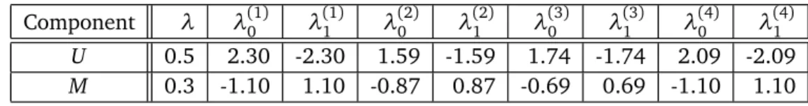
(2) Models with two-factor interactions for both U andM, i.e., ModelM₁₁. Specifications of main effects and interactions are in Table 4. Note that

λ(₁i)=−λ(₀i), λ(₀₁i j)=λ(₀₁i j)=−λ(₀₀i j), λ(₁₁i j)=λ(₀₀i j), i,j=1, 2, 3, 4.

Thus, effects and interactions at other levels can be readily derived from the one at level 0.

Table4: Speiationsofmaineetsandinterationsofmodelswithinterationsatlevel0.

Component λ λ(₀1) λ₀(2) λ(₀3) λ(₀4) λ₀₀(12) λ(₀₀13) λ(₀₀14) λ₀₀(23) λ(₀₀24) λ(₀₀34)

U 0.5 2.3 0.6 1.00 3.0 1.04 0.40 1.13 0.65 0.20 1.40

M 0.3 -1.2 -0.9 -0.66 -0.5 0.44 -0.64 -0.16 -1.08 1.08 0.32

With two different mixture models assigned for each of the six cases of data settings, we have investigated 12 simulation cases in total. Since the mixture model is for comparison vectors, we do not need to generate two original record files in each simulation case. Actually, what we need to generate are(N−Nm)comparison vectors from the loglinear model for U

andN_m comparison vectors from the loglinear model for M in each simulation case. These comparison vectors yield the 2×2×2×2 tables of 16 cells (see Table 1). Therefore, we finally need the contingency tables for U and M respectively. Note that conditional on the total count, the joint counts of all cells follow a multinomial distribution. SupposeY_i andµi

are the observed count and expected count in cell i respectively. Let N₀ be the total count. Then, conditional onP16_i=1Y_i=N₀,

R. Zhu, J. Zhang, D. Zhang, G. Yan Eur. J. Pure Appl. Math,3(2010), 141-162 155

where pi =µi P16

j=1

µj, the probability that an observed vector occurs in celli, i=1, 2, . . . , 16.

For a reference, see[2], P. 317-318. In general, we can simulate a contingency table according to (12) for a specified total count. This is the method we use to simulate data sets for six settings with mixture modelM₁₁. However, if fields are independent, we can generate four independent binary columns of length being the specified total count N0. Each column is a

series ofN0Bernoulli trials with success probability which can be readily computed according

to (12). Information of a and b will be used in the choice of initial values in the simplified method for the EM algorithm.

We apply the proposed building strategy to select a loglinear mixture model for each sim-ulation case. The significance level is set asα =5%. The following lists the model building processes and the finally selected models for all the 12 simulation cases. Due to space limita-tion, we omit the details of the estimated models.

• For the true loglinear mixture model beingM00(refer to Table 3), settings 1, 2, 3, 5 and

6 lead toM₀₀ while setting 4 yieldsM₀₀→ M₁₀. Thus, from the viewpoint of model fitting, setting 4 is a little bit overfitted with false interactions forU.

• For the true loglinear mixture model beingM₁₁(refer to Table 4), settings 1, 2, 4 and 6 proceed asM00→ M10→ M11while settings 3 and 5 result inM00→ M10. Hence,

settings 3 and 5 are a little bit underfitted without capturing the two-factor interactions forM.

Regarding the true mixture model beingM₀₀, five out of six simulation cases yield the se-lected models consistent with the true one, however, one case results in overfitting. Further investigation shows that the p-values in testingH0: M00=M10for the settinga=400 and

b=400 are 0.047(<0.05)whenN_m =40 (setting 3) and 0.105(>0.05)whenN_m =200 (setting 4). Note that setting 4 has the highest proportion of matched pairs, with half of records in each file corresponding to the same objects. This highly matching feature might cause model inflation for componentU when fields are actually independent. As to the true mixture model beingM₁₁, four out of six cases lead to models consistent with the true ones, but two cases fail to capture the two-factor interactions in the loglinear model forM, leading to underfitting for the mixture. Note that both overfitting and underfitting happen when the number of matched pairs N_m is small. Hence, empirically, it may be more difficult to find higher order interactions for theM component than for theU component in the mixture. Cu-riously, we have not observed any overfitting when the true mixture model isM11in a larger

scale investigation. These observed phenomena indicate that the proposed model building strategy may not capture the true underlying mixture model perfectly. Sometimes it yields a slight overfitting or underfitting for one of the mixture components.

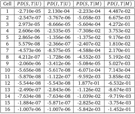
viewpoint of cell probabilities. This is to see whether or not our proposed data-driven strategy can beat or at least is equivalent to the subjective specification with naive field independence used in some record linkage software. We show the details in Table 5 for setting 5 when the true mixture model is M11. In this simulation case, the selected model by the data-driven

strategy is underfitting in theM component, not perfectly consistent with the true underlying model. In Table 5,

• P D(S,T|U) and P D(S,T|M) denote differeences in cell probabilities between the se-lected model by the data-driven strategy and the true model for componentU and M

respectively,

• P D(I,T|U) and P D(I,T|M) denote differeences in cell probabilities between the sim-plest starting modelM00and the true model for componentU andM respectively.

Table5: Comparisonsofellprobabilitiesbetweentwottedmodelsandthetruemodel,M

11,forsetting 5.

Cell P D(S,T|U) P D(I,T|U) P D(S,T|M) P D(I,T|M) 1 -2.710e-05 2.130e-04 -2.233e-04 4.487e-02 2 -2.547e-07 -3.767e-06 -5.058e-03 6.675e-03 3 2.973e-05 -8.666e-05 -5.604e-04 4.272e-01 4 2.606e-06 -2.535e-05 -7.308e-02 3.753e-02 5 2.865e-06 -1.356e-06 -1.375e-02 9.176e-03 6 5.579e-08 -2.366e-07 -2.407e-02 1.810e-02 7 -4.573e-06 -8.575e-05 -4.588e-04 2.170e-01 8 4.212e-07 -1.728e-06 -4.552e-03 5.192e-02 9 -2.060e-06 -3.412e-06 -5.084e-05 5.027e-03 10 -5.656e-08 -5.617e-08 -6.071e-04 7.143e-04 11 -5.870e-08 -1.122e-07 -9.592e-03 3.858e-02 12 -5.544e-08 -5.543e-08 1.877e-01 -6.532e-01 13 -2.490e-07 -2.843e-06 -1.126e-02 -8.674e-03 14 -7.634e-08 -7.634e-08 -1.039e-02 -9.719e-03 15 -1.884e-07 -5.871e-07 -2.825e-02 -3.754e-03 16 -1.007e-06 -1.007e-06 -5.842e-03 -1.452e-01

The smaller the absolute value in the table, the closer the corresponding cell probability is to the truth. Table 5 shows that compared with the simplest starting modelM00, the model

selected by the data-driven strategy has smaller absolute values of probability differences in almost all cells for the estimatedU component, and in the majority of cells for the estimated

R. Zhu, J. Zhang, D. Zhang, G. Yan Eur. J. Pure Appl. Math,3(2010), 141-162 157

with the naive specification of field independence (i.e., starting modelM00). Due to space

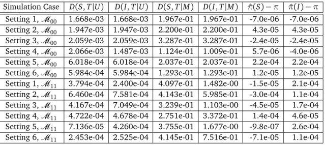
limitation, we summarize only the cell probability differences between the selected and the true models, as well as those between the fittedM00and the true model in Table 6 forU and

M respectively, using the following measures for two general loglinear mixture models:

D(M(0),M(1)|U) = X i∈all cells

|p(_i0)(U)−p(_i1)(U)|,

D(M(0),M(1)|M) = X i∈all cells

|p(_i0)(M)−p(_i1)(M)|.

Herep(_ij)is the probability of celliin modelM(j)_{. In addition, we also compare the estimated} mixing proportionπˆ(S)from the data-driven strategy andπˆ(I) from the field independence specification with the trueπ:πˆ(S)−πandπˆ(I)−π.

Table6: Overallttingomparisonsbetweentwottedmodelsandthetruemodel.

Simulation Case D(S,T|U) D(I,T|U) D(S,T|M) D(I,T|M) πˆ(S)−π πˆ(I)−π

Setting 1,M₀₀ 1.668e-03 1.668e-03 1.967e-01 1.967e-01 -7.0e-06 -7.0e-06 Setting 2,M₀₀ 1.947e-03 1.947e-03 2.200e-01 2.200e-01 4.3e-05 4.3e-05 Setting 3,M₀₀ 2.059e-03 2.059e-03 3.287e-01 3.287e-01 -2.4e-05 -2.4e-05 Setting 4,M₀₀ 2.066e-03 1.487e-03 1.124e-01 1.009e-01 5.7e-06 -4.0e-06 Setting 5,M₀₀ 6.018e-04 6.018e-04 2.037e-01 2.037e-01 2.2e-04 2.2e-04 Setting 6,M00 5.984e-04 5.984e-04 1.293e-01 1.293e-01 1.2e-05 1.2e-05

Setting 1,M11 3.794e-04 2.400e-04 4.097e-01 1.482e-00 -1.5e-05 2.1e-04

Setting 2,M11 6.460e-04 7.581e-04 4.143e-01 5.985e-01 -3.0e-04 1.1e-04

Setting 3,M₁₁ 4.167e-04 7.049e-04 3.239e-01 1.103e-00 -4.5e-05 1.7e-04 Setting 4,M₁₁ 4.722e-04 4.678e-04 2.751e-01 3.372e-01 1.4e-04 4.6e-05 Setting 5,M₁₁ 7.136e-05 4.260e-04 3.755e-01 1.677e-00 -9.8e-07 2.6e-04 Setting 6,M₁₁ 2.453e-04 2.525e-04 4.145e-01 7.516e-01 -7.1e-05 1.1e-04

Table 6 shows that when the underlying true mixture model isM₀₀, the data-driven strat-egy yields the same results as the Jaro’s method if the selected model is consistent withM00.

This means that the simplified method for the EM algorithm is equivalent to the Jaro’s method when the field independence exists, and is thus an alternative approach. However, the advan-tage of this approach is that it can handle general contingency tables with factor levels more than two.

Regarding the performance of two fitted models in Table 6, when the field independence holds, the selected models by the data-driven strategy are almost the same as the fittedM₀₀ except one overfitting case. However, they perform better than the fitted M00 when field

independence is violated.

the individual interactions in a given loglinear model in the proposed model building strategy, and it is also the partial reason why models are enlarged with a group of interactions in the building strategy in (11). Even more, for a data set simulated from a known loglinear model with three-factor interactions, the fitted model does not include these three-factor interactions although we increase the total count as many as possible in R. Therefore, in practice, it is likely to stop at a model with lower order interactions such as two-factor interactions, and this selected model may be a good approximation to the true model under the given sample size.

5. Application to a case study

We apply the proposed model building strategy to the record linkage case study at SSC 2006 (www.ss.a/douments/ase_studies/2006/reord_index_e.html).

The objective of the case study is to maintain a registry. Four completely synthetic data files named as “register”, “births”, “drivers” and “deaths” were constructed to simulate the registry for a sample of residents of the province of Prince Edward Island (PEI), Canada. The “register” file represents the population of PEI, containing a unique id, name, date of birth, and address information for residents. This is the file that we are working to maintain. The “births” file records new entrants into the population. They are persons who enter the population of interest, for example by moving into an area of interest, or attaining a certain age. The data file on births contains both present and previous address information as well as complete name and date of birth information. The “drivers” file provides moving information for registry. People living in Canada may take out their first license, get a new license (out of province) or update their present license (within a province). This file has information on name, address and date of birth. The “deaths” file contains name, address, date of birth and date of death. Note that data sources are updated independently. The main file is the “register” file which needs to be updated according to the other three files. In summary, the specific tasks include

(1) add new entrant records to “register” file from “births” file,

(2) update moving records to “register” file from “drivers” file,

(3) remove death records from “register” file according to “deaths” file.

To achieve these goals, we first need to identify common individuals in two compared files. Thus, record linkage is employed in these tasks.

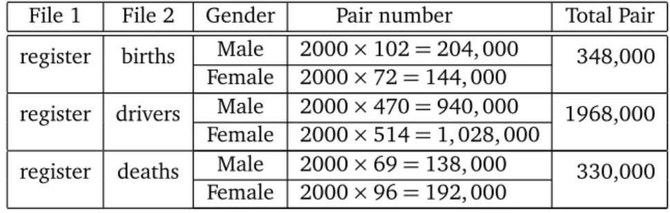
Basically, the records in these files contain common personal information such as name (first, middle and last), date of birth (day, month and year), gender, address, and so on. We adopt the gender as the blocking factor to reduce both the number of record pairs and the number of factors in the fitted models. Table 7 summarizes the total pairs in each of three tasks after the gender blocking.

R. Zhu, J. Zhang, D. Zhang, G. Yan Eur. J. Pure Appl. Math,3(2010), 141-162 159

Table7: Numbersofreordpairsbetweenomparedlesafterblokingusinggender.

File 1 File 2 Gender Pair number Total Pair

Male 2000×102=204, 000 register births

Female 2000×72=144, 000 348,000 Male 2000×470=940, 000

register drivers

Female 2000×514=1, 028, 000 1968,000 Male 2000×69=138, 000

register deaths

Female 2000×96=192, 000 330,000

name, last name and postal code as identifiers, because the date of birth seems wrong by visual check. Furthermore, we exclude the records with missing values or error values on identifiers and gender in each file. These excluded records will be manually reviewed. The simple matching of “agreement” or “disagreement” is chosen as the comparison rule. Therefore, for the comparison vectorγ= (γ1,γ2,γ3,γ4), all four fields are binary, indicating match or

non-match on identifiers. Each of the record pairs in Table 7 yields an observed comparison vector. Three contingency tables are then created for the comparison vectors, one for each task.

Next we apply the data-driven strategy to the three obtained contingency tables. The significance level is set as 5%. The selected models (in Poisson GLM formulation) are listed below.

(1) For adding new entrant records from the “births” file,γ1,γ2, γ3 andγ4 mean match or

non-match on first name, middle name, last name and date of birth respectively. The fitted model isM10with an estimated mixing proportionπˆ=4.885e−4, where theU

component is

α=12.704, α1=−6.586, α2=−3.046, α3=−5.998, α4=−10.219, α12=4.245, α13=1.819, α14=−13.911, α23=1.804, α24=0.561, α34=−14.031,

and theM component is

α=−77.456, α1=27.503, α2=27.805, α3=0.332, α4=26.410.

(2) For updating moving records from the “drivers” file, γ1,γ2, γ3 andγ4 mean match or non-match on first name, middle name, last name and postal code respectively. The fitted model isM11with an estimated mixing proportionπˆ=4.032e−4, where theU

component is

α=14.439, α1=−6.432, α2=−3.128, α3=−5.849, α4=−8.882,

α12=4.205, α13=1.427, α14=1.569, α23=1.879, α24=0.427, α34=1.807,

and theM component is

α12=27.088, α13=45.199, α14=−27.411, α23=−43.852, α24=29.412,

α34=23.367.

(3) For removing death records according to the “deaths” file,γ1,γ2,γ3andγ4mean match

or non-match on first name, middle name, last name and date of birth respectively. The fitted model isM10with an estimated mixing proportionπˆ=4.455e−4, where theU

component is

α=12.652, α1=−6.725, α2=−3.058, α3=−5.531, α4=−9.320,

α12=3.794, α13=2.159, α14=−20.402, α23=1.391, α24=−0.302, α34=−20.899,

and theM component is

α=−28.828, α1=3.570, α2=3.871, α3=4.956, α4=21.366.

In these fitted models, we see interactions among names (first, middle and last), date of birth, and postal code. Note that these four synthetic files were actually constructed from other survey sources about PEI. So more or less they reflect the local information. The reason for the interactions among names may be traced back historically on the residents’ family, origin and culture. In addition, PEI is a relatively closed island and the economy is not as active as most of other Canadian provinces. Families who are relatives might be more likely to live in a closed regions due to some reasons like traditional farming or other social activies, which could lead to the spatial patterns for surnames. Hence, these interactions are caused or confounded by the latent factors. Of course, these reasons could lead to higher order interactions, say three-factor interactions. However, with the current sample sizes, only two-factor interactions are significant enough to be included in the selected models.

We also build models for male and female block pairs separately in each task. Results are very similar and hence omitted.

It is straightforward to calculate matching weights and perform record pair partition for each task according to the corresponding selected model; this part is also omitted as it is not the focus of this paper.

6. Discussion

The simplified method for the EM algorithm is computationally effective. It also extends the Jaro’s method for a general contingency table in fitting loglinear mixture models. This method can be easily implemented in a sophisticated statistical software using existing pack-ages or functions for loglinear model fitting. We utilize R in this study. Compared with the Jaro’s method, we extend not only the factor interactions but also the number of levels of each factor. The factor is not necessarily binary. It can be more than two levels for each factor.

caused by biased opinions. Often it yields a model consistent with the true one or close to the true one. Therefore, it is more likely to result in a better partition for record linkage. However, since the proposed strategy is not a global search, the selected model may not be the best.

Future investigations regarding other testing methods and building strategies, as well as error rate investigation are under way. We welcome any real case collaboration.

ACKNOWLEDGEMENTS This research has been supported by an NSERC Discovery grant. We thank Professor Román Viveros-Aguilera at McMaster University, Canada for his helpful discussion, and Miss Yunna Song for her participation as a team member in the record linkage case study at SSC 2006. In addition, we are grateful to a referee for comments leading to an improved presentation.

References

[1] E. D. Acheson. Record Linkage in Medicine. E. & S. Livingstone Ltd., Edinburgh and London, 1968.

[2] A. Agresti.Categorical Data Analysis, Second Edition. John Wiley & Sons, Inc., Hoboken, New Jersey, 2002.

[3] J. B. Copas and F. J. Hilton. Record linkage: Statistical models for matching computer records.Journal of the Royal Statistical Society, A, 153:287–320, 1990.

[4] A. P. Dempster, N. M. Laird, and D. B. Rubin. Maximum likelihood from incomplete data via the em algorithm. Journal of the Royal Statistical Society, B, 39:1–38, 1977.

[5] M. E. Fair and P. Whitridge. Tutorial on record linkage. In W. Alvey and B. Jamer-son, editors,Record Linkage Techniques - 1997: Proceedings of an International Workshop and Exposition., pages 457–482, Arlington, VA, 1997. Federal Committee on Statistical Methodology, and Office of Management and Budget.

[6] I. P. Fellegi and A. B. Sunter. A theory for record linkage. Journal of the American Statistical Association, 64:1183–1210, 1969.

[7] M. A. Jaro. Advances in record-linkage methodology as applied to matching the 1985 census of tampa florida. Journal of the American Statistical Association, 84:414–420, 1989.

[8] M. A. Jaro. Probabilistic linkage of large public health datafiles. Statistics in Medicine, 14:491–498, 1995.

[10] M. D. Larsen and D. B. Rubin. Iterative automated record linkage using mixture models.

Journal of the American Statistical Association, 96:32–41, 2001.

[11] G. J. McLachlan and T. Krishnan. The EM algorithm and extensions. Wiley, New York, 1997.

[12] H. B. Newcombe.Handbook of Record Linkage: Methods for Health and Statistical Studies, Administration, and Business. Oxford University Press, Inc., New York, 1988.

[13] H. B. Newcombe, J. M. Kennedy, S. J. Axford, and A. P. James. Automatic linkage of vital records.Science, 130:954–959, 1959.

[14] Y. Thibaudeau. The discrimination power of dependency structures in record linkage.

Survey Methodology, 19:31–38, 1993.

[15] W. E. Winkler. Using the em algorithm for weight computation in the fellegi-sunter model of record linkage. In Proceedings of the Section on Survey Research Methods., pages 667–671. American Statistical Association, 1988.

[16] W. E. Winkler. Method for adjusting for lack of independence in an application of the fellegi-sunter model of record linkage. Survey Methodology, 15:101–107, 1989.