A mini course on additive combinatorics

(1)

1

A mini course on additive combinatorics

First draft. Dated Oct 24th, 2007

These are notes from a mini course on additive combinatorics given in Princeton University on Au-gust 23-24, 2007. The lectures wereBoaz Barak(Princeton University),Luca Trevisan (Univer-sity of California at Berkeley) andAvi Wigderson(Institute for Advanced Study, Princeton). The notes were taken by Aditya Bhaskara, Arnab Bhattacharyya, Moritz Hardt, Cathy Lennon, Kevin Matulef, Rajsekar Manokaran, Indraneel Mukherjee, Wolfgang Mulzer, Aaron Roth, Shubhangi Saraf, David Steurer, and Aravindan Vijayaraghavan.

The lectures were also videotaped, and the tapes appear on the course’s website at http://www. cs.princeton.edu/theory/index.php/Main/AdditiveCombinatoricsMinicourse

(2)

(3)

2

Szemeredi’s Regularity Lemma, and Szemeredi’s Theorem for k=3

Luca Trevisan

Scribe(s): Kevin Matulef

In this lecture we give a sketch of Szemeredi’s theorem for k=3. The proof consists of four steps. The first step, the Regularity Lemma, will be proven in a later lecture. In this lecture we explain how each subsequent step follows from the the previous one. The steps are:

1. The Regularity Lemma. Roughly, this says that every graph has a constant size approximate representation (the size of the representation depends only on the quality of the approxima-tion).

2. The Triangle Removal Lemma. This says that if a graph haso(n3) triangles, then it is possible to removeo(n2) edges and break all the triangles.

3. Szemeredi’s Theorem for k=3 for groups. 4. Szemeredi’s Theorem for k=3 for the integers.

2.1 How (3) implies (4).

For convenience, we restate the two versions of Szemeredi’s Theorem for k= 3 here:

Theorem 2.1.1 (Szemeredi’s Theorem for k= 3 for Groups). ∀δ, there exists n(δ) st ∀N ≥n(δ)

and all subsets A ⊆_Z_N where |A| ≥δN, A contains a length-3 arithmetic progression (i.e. three points a, b, c∈ZN such that b−a≡c−b mod N).

Theorem 2.1.2 (Szemeredi’s Theorem fork = 3 for the Integers). ∀δ, there exists n(δ) st ∀N ≥

n(δ) and all subsets A ⊆ {1, ..., N} where |A| ≥δN, A contains a length-3 arithmetic progression (i.e. three points a, b, c∈ {1, ..., N} such thatb−a=c−b).

To see that Theorem 2.1.1 implies Theorem 2.1.2, fixδ and letA⊆ {1, ..., N},|A| ≥δN. Think of A as a subset of Z2N, so that |A| ≥ δ₂|Z2N|. If N is large enough, Theorem 2.1.1 implies that

(6)

6CHAPTER 2. SZEMEREDI’S REGULARITY LEMMA, AND SZEMEREDI’S THEOREM FOR K=3LUCA TREVISAN there existsa, b, c∈A s.t. b−a≡c−b(mod 2N). But since a, b, c are all in the range {1, ..., N},

then b−aand c−b are both in the range{1−N, ..., N −1}. So the only way that they can be equal modulo 2N is if in factb−a=c−bwithout the mod. This proves Theorem 2.1.2, contingent on Theorem 2.1.1.

2.2 How (2) implies (3).

We begin with a formal definition of the triangle removal lemma:

Lemma 2.2.1 (Triangle Removal Lemma). For all δ, there exists = (δ) st. for every graph G

onn vertices, at least one of the following is true:

1. G can be made triangle-free by removing< δn2 _edges.

2. G has ≥n3 triangles.

In this section we see how Lemma 2.2.1 implies Theorem 2.1.1.

To prove Theorem 2.1.1, start with a group H, and a subset A ⊆H. Then construct a graph onn= 3|H|vertices by making three vertex sets, call them X, Y, Z, each with|H|vertices labeled according to H. Connect these vertices as follows:

• Connect a vertex x∈X and y∈Y if∃a∈A sty=x+a. • Connect a vertex y∈Y and z∈Z if∃c∈A stz=y+c. • Connect a vertex x∈X and z∈Z if∃b∈A stz=x+b+b.

Observe that for every choice of x ∈ H and a ∈ A, the graph has triangles of the form (x, x+a, x+a+a). These triangles are all edge disjoint, so the graph has at least |H| × |A| edge disjoint triangles. Since |A| ≥ δ|H| and |H| = n/3, this means that to make the graph triangle free we must remove at least |H| × |A|=δn2/9 edges. Using this observation and Lemma 2.2.1 with=(δ/9), we conclude that the graph has at leastn3_{= 9}_|_H_|3 _triangles.

There is a correspondence between triangles in the graph and length-3 arithmetic progression. If (x, y, z) is a triangle in the graph, then there existsa, b, c∈Asty=x+a,z=y+c, andz=x+b+b. Putting these equations together and rearranging, we get a−b=b−c. Conversely, if (a, b, c) form an arithmetic progression in A, then it easy to see that for any x, the tuple (x, x+a, x+b+b) forms a triangle in the graph. In fact, for each x ∈ H, there is a bijection between arithmetic progressions (a, b, c) and triangles of the form (x, y, z). Thus, the total number of triangles in the graph is |H|× (# of length-3 progressions inA).

Since the total number of triangles in the graph is at least n3 = 9|H|3_{, the total number}

of length-3 progression in A is at least 9|H|2_{. This is counting the “trivial progressions” where} a = b = c, but even when we exclude those progression we are left with at least 9|H|2 ₋_δ_|_H_|

length-3 progressions inA. This is positive when|H|is large enough. Thus, Theorem 2.1.1 follows from Lemma 2.2.1.

(7)

2.3. HOW (1) IMPLIES (2). 7

2.3 How (1) implies (2).

We begin with some definitions:

Definition 2.3.1. For disjoint vertex setsA, B, thedensity betweenAand B is

d(A, B) = # edges betweenAand B |A||B|

Definition 2.3.2. Two disjoint vertex sets are -regular if∀S⊆A where|S| ≥|A|, and ∀T ⊆B

where|T| ≥|B|, it holds that

|d(S, T)−d(A, B)| ≤

Informally, a bipartite graph is -regular if its edges are dispersed like a random graph’s. Lemma 2.3.3 (Szemeredi’s Regularity Lemma). ∀, t, ∃k=k(, t), k ≥t st for every graph G= (V, E) there exists a partition of G into (V1, ..., Vk) where |V1|=|V2|=... =|Vk−1| ≥ |Vk| and at

least (1−) k₂ pairs(Vi, Vj) are-regular.

Informally, Szemeredi’s regularity lemma says that all graphs are mostly composed of random-looking bipartite graphs.

We would like to show that the Regularity Lemma (lemma 2.3.3) implies the Triangle Removal Lemma (lemma 2.2.1). To see this, start with an arbitrary graphG. The Regularity Lemma says we can find a ₁₀δ-regular partition with t = 10_δ into k= k(₁₀δ,10_δ) blocks. Using this partition, we define a reduced graphG0 as follows:

• Remove all edges between non-regular pairs.

Since there are at most ₁₀δ k₂ non-regular pairs, and at most (n_k)2 edges between each pair, this step removes at most ₁₀δn2 edges.

• Remove all edges inside blocks.

Since there are k blocks, and each block contains at most n/k₂

edges, this step removes at most n_k2 ≤ δ

10n

2 _edges.

• Remove all edges between pairs of density less than δ₂.

There are at most ₂δ(n_k)2 edges between a pair of density less than δ₂, and at most k₂ total such pairs, so this step removes at most ₂δn2 edges.

In total the reduced graph G0 is at most ₁₀δ +₁₀δ +δ₂ < δ far from the original graphG. Thus ifG0 contains no triangle, the first condition of the Triangle Removal Lemma is satisfied (since all the triangles can be removed from G by breaking ≤ δn2 edges). For the remainder of the proof then, we assume thatG0 does contain a triangle, and we wish to show that the second condition of the Triangle Removal Lemma is satisfied (i.e. there must by≥n3 triangles inG).

If G0 does contain a triangle, it must go between three different blocks, call them A,B, and C. Let m =n/k be the size of the blocks. Since G0 does not contain any edges between low-density pairs of blocks, we know that if there is an edge betweenAandB, then in fact there must be many edges.

(8)

8CHAPTER 2. SZEMEREDI’S REGULARITY LEMMA, AND SZEMEREDI’S THEOREM FOR K=3LUCA TREVISAN More quantitatively, we claim that at most m/4 vertices in A can have≤ δ

4m neighbors inB.

Otherwise, there would be a subset ofA, call itA0, where|A0| ≥ |A|/4, such thatd(A0, B)≤ δ₄. This violates the conditions of the Regularity Lemma, since |d(A, B)−d(A0, B)| ≥ δ₄ ≥ ₁₀δ . Likewise, the same argument shows that at mostm/4 vertices inA can have ≤ δ₄m neighbors in C.

Since at most m/4 vertices in A can have ≤ ₄δm neighbors in B, and at most m/4 vertices in

A can have≤ δ

4m neighbors inC, there must be at leastm/2 vertices in A that have both≥ δ 4m

neighbors in B and ≥ δ

4m neighbors in C.

Consider a single such vertex from A. LetS be its neighbor set inB and T be its neighbor set in C, where |S| ≥ δ

4m and |T| ≥ δ

4m. How many edges go between S and T? Since d(B, C) ≥ δ

2, and B and C are δ

10-regular, the number of edges going between S and T must be at least

(δ₂ − δ

10)|S||T| ≥ δ

4|S||T| ≥ δ3

64m

2_{. Thus a single vertex from} _A _{with high degree in both}_B _and _C

accounts for at least δ₆₄3m2 triangles in G0. Since there are at least m/2 such vertices from A, the total number of triangle must be at least ₁₂₈δ3 m3 = ₁₂₈δ3_k3n3, which is what we wanted to show.

2.4 Brief Sketch of (1)

In this section we provide a brief sketch of the Regularity Lemma, the only remaining piece of the proof of Szemeredi’s Theorem for k= 3. A more detailed proof will be given in a later lecture.

To prove the Regularity Lemma, we start with an arbitrary partition of the graph G into

t subsets. If this partition is -regular, then we are done. Otherwise, we iteratively refine the partition until we get one that is-regular. We do this as follows:

If a partition is not -regular, that means there exist at least ₂t

non-regular pairs Vi, Vj. Let Si and Tj be witnesses to the non-regularity of Vi, Vj; in other words, Si ⊆ Vi,|Si| ≥ |Vi| and

Tj ⊆Vj,|Tj| ≥|Vj|where|d(Si, Tj)−d(Vi, Vj)|> . We refine the partition by subdividing all the subsets into intersections of Vi, Vi\Si, Vj, Vj\Tj over all non-regular pairs (i, j) (we actually even

further refine the partition so that the resulting sets have equal size). To analyze this process, we examine the quantity P

i,j

|Vi||Vj|

n2 d2(Vi, Vj). This can be thought of as the variance of the densities between the sets containing two randomly chosen vertices. One can show that this quantity always increases upon refinement, and each iteration of the above process increases it by at least poly(). Since the quantity is at most 1, the refinement process must terminate after poly(1) iterations.

(9)

3

The Sum Product Theorem and its Applications

Avi Wigderson

Scribe(s): Aaron Roth and Cathy Lennon

Summary: This lecture contains the statement of the sum-product theorem and a broad survey of its applications to many areas of mathematics. Finally it sketches a proof; a full proof of the sum-product theorem is contained in the next lecture.

3.1 Preliminaries and Statement of the Sum-Product Theorem

LetFbe a field, and letA⊆Fbe an arbitrary subset. In particular,Ais not necessarily a subfield, and so is not necessarily closed under either field operation. We may therefore wish to study how closeA is to a closed set under each field operation. The following definitions capture this:

Definition 3.1.1. For A⊆F, thesumset A+Ais:

A+A={a+a0 :a, a0 ∈A} Definition 3.1.2. For A⊆_F, theproduct set A×Ais:

A×A={a×a0 :a, a0 ∈A}

If Ais a subfield ofF, then|A+A|=|A×A|=|A|. IfA is not closed under some operation·, then|A·A|>|A|. In principle, |A·A|can be as large as Ω(|A|2_{), but we may be interested in sets} A such that|A+A|or|A×A|is small.

3.1.1 Over the Reals

Example 3.1.3. ForF=R andA={1,2,3, . . . , k} we have:

• |A+A|<2|A|(pairwise addition of elements in Ayields integers in {2, ...,2k} • |A×A|= Ω(|A|2₎

(10)

10CHAPTER 3. THE SUM PRODUCT THEOREM AND ITS APPLICATIONSAVI WIGDERSON For F=Rand B={1,2,4, . . . ,2k} we have:

• |B×B| ≤2|B|(since this is {2a:a∈ |A+A|})

• |B+B|= Ω(|B|2_{) (Like the set of all length-}_k_{binary strings with norm 2)}

In these examples, either the sumset or the product set is small, but not both. ForF=R, does there exist an A ⊂R for which max{|A+A|,|A×A|}is ‘small’ ? The sum-product theorem over the reals tells us that there is not:

Theorem 3.1.4 (Sum Product Theorem forF=R[ES83a]). ForF=R,∃ >0such that ∀A⊂F

either:

1. |A+A| ≥ |A|1+

2. |A×A| ≥ |A|1+

The bestknown in the above theorem is 4/3, but it is conjectured that it holds for= 2−o(1).

3.1.2 Over a Finite Field

SupposeF is a finite field. Can Theorem 3.1.4 still hold? Not quite as stated:

• IfA⊂Fsuch that|A| ≥CFfor some constantC, neither|A+A|nor|A×A|can exceed |A| by more than a constant factor. We must therefore have a condition that Ais not ‘too big.’ • IfAis a subfield ofFthen it is closed under both field operations, and so|A+A|=|A×A|=

|A|. We must therefore have a condition that F contains on subfields.

The following version of the sum-product theorem holds for finite fields Fp for p prime (this

restriction guarantees that there are no nontrivial subfields – variants of this theorem are possible for other fields with small subfields.)

Theorem 3.1.5 (Sum Product Theorem for F = Fp [BT04][Kon03]). For F = Fp for p prime,

∃ >0 such that∀A⊂F with |A| ≤ |F|.9, either:

1. |A+A| ≥ |A|1+

2. |A×A| ≥ |A|1+

The best known in the above theorem is.001, and it is known that cannot be larger than 3/2.

3.2 Applications

The sum-product theorem has wide ranging applications. In this section, we survey various fields of mathematics and give theorem statements that were state-of-the-art before application of the sum-product theorem, and then the corresponding improvement possible with the sum-product theorem.

(11)

3.2. APPLICATIONS 11

3.2.1 Combinatorial Geometry

Consider the geometry of a planeF2. Let P be a set of points in F2 of cardinality n, and let Lbe a set of lines inF2 also of cardinalityn. A natural quantity to study is

I ={(l, p) :l∈L, p∈P such that point p lies on line l}

the set of incidences of points inP on lines inL. Using only simple combinatorial facts about lines and planes we may prove the following simple bound:

Theorem 3.2.1.

|I| ≤O(n3/2)

Proof. Let

δp,l=

1, if point p lies on line l; 0, otherwise.

Letf(l) =P

p∈P δp,l denote the number of points incident on linel and letg(p) =Pl∈Lδp,l denote

the number of lines incident on a pointp. Node that|I|=P

p∈Pg(p) =

P

l∈Lf(l). then:

|I| = X

l∈L f(l)

= X

l∈L

1·f(l) ≤ √n·

s X

l∈L f(l)2

= √n·

s X

l∈L

(X

p∈P

δp,l)(X

p∈P δp,l) = √n·

s X

p,p0_∈_P

X

l∈L δp,lδp0_,l

= √n·

s X

p∈P

g(p) +X

p6=p0

X

l∈L δp,lδp0_,l ≤ √n·p|I|+n2

where the first inequality follows from Cauchy-Schwartz, and the second follows from the fact that there can be at most one line incident to any two distinct points, and there are fewer thann2 pairs of points. Solving for|I|we get the desired bound.

For F=Ra tighter non-trivial bound is possible without the sum-product theorem: Theorem 3.2.2 ([?],[Ele97]). For F=R|I| ≤O(n4/3)

With the sum-product theorem, a big improvement is possible (this is a non-trivial consequence of a statistical-version of the sum-product theorem):

(12)

12CHAPTER 3. THE SUM PRODUCT THEOREM AND ITS APPLICATIONSAVI WIGDERSON

3.2.2 Analysis

Consider the following question which has many applications in analysis/PDE: what is the smallest area of a figure which contains a unit segment in every direction? 1

In the Reals Besicovitch proved:

Theorem 3.2.4 ([Bes63]). One can construct S ⊆ R2 with arbitrarily small area such that S

contains a unit segment in every direction.

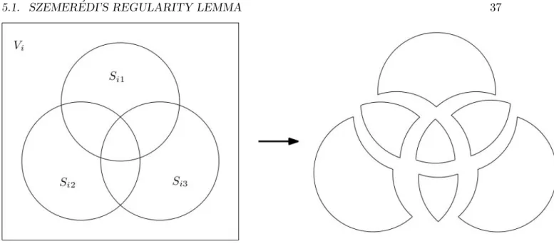
The construction is as follows: begin with a square of side length 2 with center Oand add lines across the diagonals, partitioning it into four isosceles right triangles with hypotenuse of length 2 with common vertex O. Partition each hypotenuse into n equally sized segments, where the value of n depends on how small of an area is desired. For each endpoint, draw a line from O to the endpoint. This further partitions the square into 4n “elementary triangles”. The resulting object looks like:

By constructing the figure like this, it is clear that considering each of the 4n elementary triangles and all possible segments with one endpoint at O and the other at a point in the base of the triangle, then the collection of all such segments for all triangles will have a range of 360◦ and each such segment will have a length of at least 1. Therefore,the collection of these 4n triangles contains a unit segment in all possible directions. Of course, the area of this square is quite large.

1

Examples of such figures are a circle of radius 1 (area=π/4≈.78) and an equilateral triangle of height 1 (area=

1 √

3 ≈.58). It was also (falsely) conjectured that the hypocycloid inscribed in a circle of diameter 3/2 was the figure

(13)

3.2. APPLICATIONS 13 They key to his construction is following observation: arbitrary translations of the elementary triangles does not affect which unit segments are contained within the triangles. By translating them in such a way that they overlap, we can decrease the total area of the figure while maintaining the property of containing a unit segment in all directions.

We describe the translations for the bottom triangle, but the same procedure may be plied to the other three, resulting in a solution to the problem. For any integerp≥2 consider the sequence of triangles ∆2, ∆3,...,∆p, where each is a right isosceles triangle, and ∆k has height k/p, base

partitioned into 2k−2 segments, and a line joining each segment endpoint to the common vertex. Thus triangle ∆k consists of 2k−2 elementary triangles. Each ∆k+1 can be constructed from ∆k

by bisecting each of the elementary triangles of ∆k through their base, and scaling each so that

it now has height k+ 1. This will create a series of overlapping triangles that can be translated to construct ∆k+1. This process is known as “bisection and expansion”. By starting with triangle

∆2, and then using this technique repeatedly, after p−2 steps, we will have 2k−2 overlapping

elementary triangles which can be translated to form ∆p. Analysis of the process of bisection and

expansion shows that each step increases the total area by at most _p12 and so at the final step the constructed object S1 has area 2_p. Choosing p >8/will make the area of S1 less than /4. Doing

this for each of the four original right triangle results in a figure of area at most. Since this figure consists of translations of the elementary triangles described above, it contains a unit segment in every direction.

One can also ask this question for Rd for d > 2 or for measures other than the Lebesque measure. A third variation is to consider this question for finite fields, and it is in this case that the sum-product theorem gives interesting results.

In Finite Fields

Call a set S ⊂ (Fp)d a Kakeya set if S contains a line in all possible directions (for large p). By

this we mean that for all b ∈Fdp\ {0} there is an a∈Fdp such that a+tb∈ S for all t∈Fp. Any

particular line is of the form a+tb and since t∈ Fp, each line contains p points. Define B(d) to

be the smallest r such that there exists a Kakeya set S with|S|= Ω(pr). It has been conjectured thatB(d) =d.

Before the sum-product theorem, the following was known: Theorem 3.2.5. (Trivial) B(d)≥d/2

Theorem 3.2.6 ([Wol99]). B(d)≥d/2 + 1

However, one can use the sum-product theorem to show that: Theorem 3.2.7 ([BT04]). B(d)≥d/2 + 1 + 10−10

We will show the trivial bound of B(d)≥d/2. The proof relies on the following fact: if P is a collection of points in Fdp and L is a collection of lines in Fdp, then

{(p, l)∈P ×L:p∈L}| ≤min(|P|12|L|+|P|,|P||L| 1 2 +|L|)

To apply this, let P be any set of points inFdp which contains lines in every possible direction,

(14)

14CHAPTER 3. THE SUM PRODUCT THEOREM AND ITS APPLICATIONSAVI WIGDERSON that |L| ≥ p_pd₋−₁1. Since we assume that all of the points in each line lie in P, and since each line hasp points, we have

p|L|=|{(p, l)∈P ×L:p∈L}| ≤ |P||L|12 +|L| =⇒ |P| ≥ |L|12(p−1)≥(p

d₋₁ p−1 )

1

2(p−1) = ((pd−1)(p−1)) 1

2 = (pd(p−1− 1

pd−1 +

1

pd))

1

2 ≥pd/2 So any Kakeya setS satisfies|S| ≥pd/2 and henceB(d)≥d/2.

3.2.3 Number Theory

ForF=Fp a finite field of prime order, letGbe a multiplicative subgroup ofF∗. Define the fourier coefficient atarelative to Gto be:

Definition 3.2.8 (Fourier coefficient ata).

S(a, G) =X

g∈G ωa·g

A natural quantity to study is the maximum fourier coefficient of any element in F∗:

S(G) = max

a∈F∗

|S(a, G)| We may provide a trivial bound:

Theorem 3.2.9.

S(G)≤ |G|

Proof.

S(G) = max

a∈F∗

|X

g∈G ωa·g|

≤ max

a∈F∗

X

g∈G

|ωa·g|

= X

g∈G

1 = |G|

We would instead like to show that S(G)≤ |G|1−_.

Without the sum-product theorem, this was demonstrated for |G| ≥ p1/2 [Wol99], |G| ≥ p3/7

[HB96], and|G| ≥p1/4 [KS99].

Using the sum-product theorem, more general results can be derived:

Theorem 3.2.10 ([BT04]). ForF=Fp withp prime, and|G| ≥pδ, S(G)≤ |G|1−(δ)

Theorem 3.2.11 ([BK06]). For F=Fp withp prime, and |G| ≥pδ, S(Gk(δ))≤ |Gk|1−(δ)

(15)

3.2. APPLICATIONS 15

3.2.4 Group Theory

Suppose that H is a finite group, and T is a set of generators for H. We can then study the structure of H with respect to T:

Definition 3.2.12 (Cayley Graph). Cay(H;T), the Cayley Graph of H and T is the graph with vertex setV =H, and edge setE={u, v:u·v−1∈T}. That is, the vertex set is the set of group elements, with edges corresponding to walks we can take among group elements by multiplying by the generators in T.

One interesting feature of a Cayley graph is its diameter Diam(H;T), the longest path between any two group elements in Cay(H;T). If Cay(H;T) is an expander graph, then the second largest eigenvalue over the matrix defining the markov process of a random walk over Cay(H;T),λ(H;T)≤ 1−, and so its diameter isO(log|H|).

ForH = SL(2, p), the group of 2×2 invertible matrices overFp, Selberg, Lubotsky Phillips and

Sarnak, and Margulis showed without the sum-product theorem a few sets of generatorsT for which Cay(H;T) is an expander [Sel65] [LS86] [Mar73]. Using the sum product theorem, Helfgott showed that for all T, the diameter of Cay(H;T) is < polylog(|H|) [Hel]. Also using the sum-product theorem, Borgain and Gamburd showed that for randomT with|T|= 2, Cay(H;T) is an expander (with diameter O(log|H|)) with high probability [BG06]. [BG06] also show that if < T > is not cyclic inH =SL(2,Z), then Cay(H;T) is an expander.

3.2.5 Randomness Extractors and Dispersers

Randomness is a powerful tool used in many areas of computer science, and has practical applica-tions because randomness appears to be prevalent in our physical experience of the world. However, theoretical applications often require uniform random bits, whereas when we observe randomness in nature, it is not of this clean form. We may have access to a random variable X with high entropy (in the sense that it would take many uniform random bits to sample fromX), but that is far in statistical distance from the uniform distributionUn – and perhaps the exact distribution of

X is unknown. If S is a such a class of probability distributions over {0,1}n_{, then}_X _∈_S _{is often}

called a ‘weak source of randomness’.

In order to make use of X in applications that require uniform random bits, we would like extractors and dispersers:

Definition 3.2.13((S, )-Disperser). A functionf :{0,1}n_{→ {}₀_,₁_}m_{for which all}_X_∈_S_satisfies:

|f(X)| ≥(1−)2m

is an (S, )-disperser. That is,f(X) is a distribution with large support (although is not necessarily distributed close to uniform).

Definition 3.2.14 ((S, )-Extractor). A function f : {0,1}n _{→ {}₀_,₁_}m _{for which all} _X _∈ _S

satisfies:

kf(x)−Umk₁ ≤

is an (S, )-disperser. That is,f(X) is -close to the uniform distribution (and in particular, must have large support).

(16)

16CHAPTER 3. THE SUM PRODUCT THEOREM AND ITS APPLICATIONSAVI WIGDERSON The existence of extractors and dispersers is a Ramsey/Discrepancy theorem, but their explicit polynomial time construction is an important research area. Extractors and dispersers can be either randomized (seeded), or deterministic. It is easy to see that there cannot be deterministic constructions that work with all high entropy sources X, but we can avoid needing any uniform random bits if we make some assumption about the structure ofS.

For example, let S = Lk, the set of affine subspaces of Fn2 of dimension ≥ k. Say that f is

optimal if m = Ω(k) and = 2−Ω(k) (information theoretic bounds tell us we cannot hope that

f(X) has higher entropy than X). Before the use of the sum-product theorem, it was known via the probabilistic method that there exist optimal affine extractors for all k ≥ 2 logn. Explicit constructions for such extractors were known only for k≥n/2. Using the sum-product theorem, better results are possible: [BW05] give an explicit construction for an affine disperser with m= 1 for allk≥δn. [Bou07] gives an explicit construction for an optimal affine extractor for allk≥δn. [GR05] give extractors for large finite fields of low dimension.

Alternately, we may considerS =Ik ={(X1, X2) :X1, X2∈ {0,1}nindependent, H∞(Xi)≥k}

whereH∞(Xi)≥k implies that no element inXi has probability greater than 2−k. For simplicity, it is helpful to think about Xi as the uniform distribution over a support of k elements. Again, f(X1, X2) cannot have higher entropy than (X1, X2), f is optimal if m = Ω(k) and = 2−Ω(k).

Before the sum-product theorem, Erdos (using the probabilistic method) showed that there exists an optimal 2-source extractor for all k ≥ 2 logn in proving the existence of Ramsey Graphs2. [CG88] and [Vaz87] gave an explicit construction for an optimal 2-source extractor for allk≥n/2. Using the sum-product theorem, (slightly) better results are possible: [Bou07] gives an explicit optimal 2-source extractor for k ≥.4999n. [BW05] give an explicit 2-source disperser for m = 1 and k ≥δn (giving new constructions for bipartite Ramsey graphs), and [BW06] give an explicit 2-source disperser for m= 1 andk≥nδ.

A Statistical Version of the Sum Product Theorem

The sum-product theorem tells us about the size of sets, and so is useful in constructing dispersers from a constant number of independent sources3. To construct extractors, however, which require not only thatf(A) have large support, but also that it be almost uniformly distributed, we would like a statistical analogue of the sum-product theorem. Intuitively, we would like a statement about the size ofAin terms of its entropy. There are several measures we might consider: H0(A) =

|support(A)| is simply the measure we have been using for the standard sum-product theorem. Shannon entropy HShannon = Pi∈A−pilogpi is one possibility. A stronger measure is H2(A) =

−log||A||2≈H∞(A) = mini∈A−log(pi). Note that we have: H2≤HShannon≤H0.

We may rephrase our existing result over Fp:

2

A Ramsey graph has no clique and no independent set of size k. Note that a two-source disperser for Ik with

m = 1 f : {0,1}2n _{→ {}₀_,₁_} _{provides a construction for a bipartite Ramsey graph. Let the graph consist of two} parts, each consisting of 2nvertices, corresponding to the binary strings of lengthn. For two verticesx, yin different parts, let there be an edge (x, y) if f(x, y) = 1. In any two subsetsS, T for|S|,|T| ≥k in different parts, we are guaranteed by the definition of a disperser that|f(S, T)|>1⇒f(S, T) ={0,1}since we may consider S andT to be the uniform distribution overkelements. Therefore, between any two subsets|S|,|T| ≥kin different parts, there are always edges, but never all of the possible edges, giving us a bipartite Ramsey graph.

3

Letf(x, y, z) =x×y+z. As a corollary of the sum-product theorem, we know that |A×A+A| ≥ |A|1+ for some constant. So long as|A| ≥Fδpfor some constantδ, by composingfwith itself a constant number of times to obtaing, we haveg(A, . . . , A) =Fp, and so we have a disperser.

(17)

3.2. APPLICATIONS 17 Theorem 3.2.15 (Sum Product Theorem Over Fp [BT04] [Kon03]). There exists an ≥0 such

that for all A⊆_F_p such that H0(A)≤.9 logp, either:

1. H0(A+A)>(1 +)H0(A) or

2. H0(A×A)>(1 +)H0(A).

We would like an identical result in which we could replaceH0 withH2 (orH∞), but this is not

possible. In particular, for every prime fieldF, there is a distribution uniform over a subset ofFof size 2k(withk <0.9 logp) such that bothA+AandA×Aput a constant probability over a set of size at mostO(2k)4. This givesH∞(A) =k,H∞(A+A)≤k+ log 1/candH∞(A×A)≤k+ log 1/c

for some constant c, which violates our desired sum-product theorem. An analogous theorem is possible, however, if we replace sums and products with a convolution. Again, rephrasing our original theorem:

Theorem 3.2.16 ([BT04] [Kon03]). There exists an ≥ 0 such that for all A ⊆ Fp such that H0(A)≤.9 logp:

H0(A×A+A)>(1 +)H0(A)

Now a statistical analogue is possible, as proven by Barak, Impagliazzo, and Wigderson: Theorem 3.2.17 ([BW04]). There exists an ≥ 0 such that for all A ⊆ Fp such that H2(A) ≤ .9 logp:

H2(A×A+A)>(1 +)H2(A)

Suppose that A, B, C are independent distributions overFp. Let the rate of distributionX be r(X) =H2(X)/logp, and let r= min(r(A), r(B), r(C)). [BW04] show the following:

There exists a constant >0 such that: • Ifr ≤0.9, thenr(A, B, C)≥(1 +)r

• Ifr >0.9, thenr(A, B, C) = 1.

Given this, and the statistical analogue of the sum-product theorem, we may construct extrac-tors in the way that we were able to construct dispersers. We define:

• f1(A1, A2, A3) =A1×A2+A3

• ft+1(A1, A2, . . . , A3t+1) =f1(ft(A₁, . . . , A₃t), ft(A₃t₊₁, . . . , A₂_·₃t), ft(A₂_·₃t₊₁, . . . , A₃t+1)) By composing f1 with itself t times, we are able to convert 3t sources with entropy H2(A) to a

single source with entropy at least (1 +)tH2(A). Using this construction, [BW04] give optimal

explicit constructions for extractors over the set

S ={(A1, . . . , Ac) :Ai independent over {0,1}n withH2(Ai)> k}

fork =δn and c= poly(1/δ) Note that for δ >0 a constant, this gives an extractor given only a

constant number of independent input sources. Without using the sum-product theorem, Rao gets a stronger result, giving an explicit construction for optimal extractors over S with k = nδ and

c= poly(1/δ) [Rao06]. 4

LetAput probability 1/2 on an arithmetic progression, and probability 1/2 on a geometric progression. Then, as we saw above,A+Awill have probability 1/2 on a set of size 2|A|, andA×Awill have probability 1/2 on a set of size 2|A|, which is what we need.

(18)

18CHAPTER 3. THE SUM PRODUCT THEOREM AND ITS APPLICATIONSAVI WIGDERSON Definition 3.2.18 (Condenser). For X a distribution on {0,1}n_{, and} _r₍_X_{) =} _H

2(X)/n, then fc : {0,1}n → ({0,1}m)c is a condenser if there exists a constant > 0 such that for all X with r(X)≤.9:

∃c >0 :r(fc(X))≥(1 +)r(X)

Intuitively, r is a measure of how close to uniform X is. fc takes a weak random variable, creates

a random variable over a possibly smaller space that is closer to uniform.

Using the sum product theorem, [BW05] give a condenser that iteratively boosts r = δ to

r= 0.9 with c= poly(1/δ) for m= Ω(n). For constant δ therefore,c is constant.

3.3 Proof Sketch of the Sum-Product Theorem

Recall the statement of the sum-product theorem:

Theorem 3.3.1 ([BT04]). Let F =Fp, then for all δ < .9 there exists an >0 such that for any A⊂F satisfying |A|=|F|δ_{, either} _|_A₊_A_{| ≥ |}_A_|1+ _or _|_A_×_A_{| ≥ |}_A_|1+_.

This theorem will be a consequence of the following two lemmas.

Lemma 3.3.2. There exists a rational expression R0 such that for all A, |R0(A)|>|A|1+δ.

where a rational expressionR(A) is a rational function inA, for exampleR(A) = (A+A−A×

A)/(A×A×A).

Proof. Define the rational expressionR0(A) := (A0−A0)/(A0−A0) =A00, whereA0 := (A−A)/(A− A). Also, define δ0, δ00 to be the values such that |A0| = |F|δ0

and |A00| = |F|δ00

. Then we claim that R0 is the desired rational expression. This will follow from the following claim (to be proven

subsequently): if δ ∈ (1/(k+ 1),1/k) then δ0 > 1_k. We know that there is some k such that δ

is in the open interval (1/(k+ 1),1/k), (note here the strict inclusion since |F|1k,|F|

1

k+1 6∈_N _but |A| ∈N). Applying the lemma twice gives that δ00>1/(k−1) and then

δ(1 +δ)< 1 k ∗

k+ 1

k =

k+ 1

k2 < k+ 1

k2₋₁ =

1

k−1 < δ 00

Putting this together gives

|F|δ(1+δ)_<_|_F_|δ00₌_|_R 0(A)|

=⇒ |R0(A)|>(|F|δ) 1+δ

=|A|1+δ which is what we wanted.

It is left to prove the claim: assume otherwise, ie that δ0 < 1_k. Construct a sequence s0 =

1, s1, ..., sk∈F such that eachsj satisfiessj 6∈s0A0+s1A0+...sj−1A0. It is always possible to find

such an sj when j ≤kbecause otherwise this would imply that s0A0+...sj−1A0 =F =⇒ |A0|>

|F|j−11_{, contradicting our assumption that} _δ0 _< 1

k.

Next, define a function g :Ak+1 → F by g(x0, ..., xk) = Psixi. By our choice of k, we have

|A|k+1 _>_|_F_|_{, so}_g _{cannot be injective, and so there exists}_x₆₌_y _{such that}P

sixi=g(x) =g(y) =

P

siyi. Choose j to be the largest index where xj and yj differ. Then P

sixi = P

siyi =⇒

P

si(xi −yi) = 0 =⇒ Pi≤jsi(xi−yi) = 0 =⇒ sj = Pi<jsi(xi−yi)/(yj −xj). Each (xi− yi)/(yj−xj)∈A0 and sosj =P

i<jsi(xi−yi)(yj−xj)∈s0A

0₊_s

(19)

3.4. CONCLUSION 19 Lemma 3.3.3. If |A+A|< |A|1+ _and _|_A_×_A_| _< _|_A_|1+ _{then for all} _R _{there exists a} _c ₌ _c₍_R₎

such that there is some B ⊆A with |B|>|A|1−c _and_|_R₍_B₎_|_{< B}1+c_.

We list only the ingredients for proving Lemma 2. A full proof will be given in the next lecture. LetG be an abelian group,A⊆G, >0 arbitrary, then the following theorems hold:

Theorem 3.3.4 ([Rao06]). |A+A|<|A|1+ ₌_{⇒ |}_A₋_A_|_<_|_A_|1+2

Theorem 3.3.5 ([Plu69],[Rao06]). |A+A|<|A|1+ ₌_{⇒ |}_A₊_kA_|_<_|_A_|1+k

Theorem 3.3.6 ([BS94], [Gow98]). ||A +A||−1 _< _|_A_|1+ ₌_⇒ _∃_A0 _⊆ _A,_|_A0_| _> _|_A_|1−5 _but

|A0+A0|<|A0|1+5_.

[The theorem now follows from these lemmas: assume for contradiction that the theorem is false, ie that there is some δ < .9 such that for all > 0 there is some set A, |A| = |F|δ _with

both |A+A| ≤ |A|1+ _and _|_A_×_A_{| ≤ |}_A_|1+_{. Let} _R

0 be as in LEMMA 1. Now A satisfies the

hypotheses of LEMMA 2 and so considering R=R0, there is ac,B with|B|>|A|1−c such that

|B|1+δ_<_|_R

0(B)|<|B|1+c]

3.4 Conclusion

What we should take away from this survey lecture is that the sum-product theorem, despite having a simple statement, is fundamental, and has applications to many areas of mathematics (many more than have been touched upon here). It has proven to be useful in computer science, and presumably has further potential. We have touched upon the sum-product theorem overRandFp for primep,

but it has other extensions: for example, over rings.

Unresolved questions about the sum-product theorem include determining the optimal value for

. Over the reals, it is believed to be 1. It is known that over finite fields, we must have≤1/2. Open questions for which the sum-product theorem may prove useful include the construction of an extractor for entropy < .4999n, and the construction of a disperser for entropy << no(1).

(20)

(21)

4

Proof of the Sum-Product Theorem

Boaz Barak

Scribe(s): Arnab Bhattacharyya and Moritz Hardt

Summary: We give a proof of the sum-product theorem for prime fields. Along the way, we also establish two useful results in additive combinatorics: the Pl¨unnecke-Ruzsa lemma and the Balog-Szemer´edi-Gowers lemma.

4.1 Introduction

Given a finite set A ⊂_Z, let A+A def= {a+b :a, b ∈ A} and A·A def= {a·b :a, b ∈ A}. Then, the sum-product theorem states that either A+A or A·A is a large set; more precisely: there exists an > 0 such that max{|A+A|,|A ·A|} ≥ |A|1+ _{for any set} _A_{. The two contrasting}

situations of a set having a large doubling and a set having a large squaring are realized by a geometric progression and an arithmetic progression respectively. If A is a geometric progression of length n, then |A·A| ≤O(n) while |A+A| ≥Ω(n2). On the other hand, if A is an arithmetic progression of length n, then |A+A| ≤O(n) while|A·A| ≥Ω(˜ n2). So, the sum-product theorem can be thought of as roughly saying that any set is either “close” to an arithmetic progression or a geometric progression.

The sum-product theorem for integers was formulated by Erd¨os and Szemer´edi [ES83b] who conjectured that the correctis arbitrarily close to 1. The theorem for= 1₄ was proved by Elekes in [Ele97]. Here, though, we are going to examine the sum-product theorem for finite fields. That is, the case when A is a subset of a finite field F. Clearly, the relationship between |A+A| and |A·A| is uninteresting when A equals F or, in general, whenA is any subfield of F because then, |A+A|=|A·A|=|A|. Therefore, in order to avoid trivialities as well as technical complications, we are going to insist thatFbe a prime field (so that it does not contain any proper subfield) and that|A|be significantly smaller than|_F|(so thatAis not the entire field). In such a setting, where |A| < |_F|0.9_{, [BT04] and [Kon03] proved the sum-product theorem with} _≈ ₀_._{001. We base our}

exposition on [Gre05, TV06, BW04].

(22)

22 CHAPTER 4. PROOF OF THE SUM-PRODUCT THEOREM BOAZ BARAK

4.2 The Sum-Product Theorem for Prime Fields

Theorem 4.2.1 (Sum-Product Theorem). Given F a prime field, A ⊆F with |A| < |F|0.9, then

there exists >0 such that max{|A+A|,|A·A|} ≥ |A|1+_.

Our proof for Theorem 4.2.1 is based on two key lemmas. Intuitively, the first lemma will say that if both |A+A|and |A·A| are small, then so is |r(A)|where r(·) is any rational expression. The second lemma will say that for a particular rational expression, r∗(·), if |A+A|is small, it is true that |r∗(A)| is large. So, if both|A+A|and |A·A|are small, the two lemmas together will yield a contradiction.

In truth, the lemmas that we can actually prove are not as strong as those described in the above paragraph, but they suffice for the proof.

Lemma 4.2.2. For any0< ρ <1, if |A·A| ≤ |A|1+ρ_and_|_A₊_A_{| ≤ |}_A_|1+ρ_{, then for every rational}

expression r(·), there existsB ⊆A such that|B| ≥ |A|1−O(ρ) _and _|_r₍_B₎_{| ≤ |}_A_|1+O(ρ)_.

Lemma 4.2.3. For prime field F andA⊆Fwith |A| ≤ |F|0.9 and |A+A| ≤ |A|1.1,

A

AA−AA

A−A +A

≥ |A|1.1

Theorem 4.2.1 now follows simply from the two lemmas.

Proof of Theorem 4.2.1 from Lemma 4.2.2 and Lemma 4.2.3. For the sake of contradiction, sup-pose there is anA⊆_Fsuch that |A| ≤ |_F|0.9 _but_|_A₊_A_| _and_|_A_·_A_|_{are both less than}_|_A_|1+ _for

any arbitrarily small constant > 0. By Lemma 4.2.2, there is an absolute constant c for which there existsB ⊆A with|B| ≥ |A|1−O() _{such that}

B

BB−BB B−B +B

≤ |A|

1+O() _{≤ |}_B_|1+c_{. Also,}

note that|B+B| ≤ |A+A|<|A|1+_{≤ |}_B_|1+O()_{. So, by Lemma 4.2.3,} B

BB−BB B−B +B

≥ |B|

1.1_.

Therefore, c ≥ 0.1 which means ≥ 0.1/c, a contradiction to the fact that can be arbitrarily close to 0.

What remains now is to prove Lemma 4.2.2 and Lemma 4.2.3.

4.3 Two Useful Tools

In order to prove Lemma 4.2.2 and Lemma 4.2.3, we will establish two generally useful tools: the Pl¨unnecke-Ruzsa lemma and the Balog-Szemer´edi-Gowers lemma. Both of these results hold when the set elements are from an arbitrary abelian group. So, any true statement made in this section about sums and differences of elements of a set implies a corresponding true statement about products and quotients (simply by changing the name of the group operation).

4.3.1 The PR Lemma

The Pl¨unnecke-Ruzsa (PR) lemma states that ifA and B are of equal size and if|A+B|is small, then|n1A−n2A+n3B−n4B|is also small wheren1, n2, n3, n4 are positive integers. So, it cannot

be the case that |A+B|is small but |A+B+B|is large if Aand B are of equal size. Note that such a statement has the flavor of Lemma 4.2.2 but it involves just one operation.

(23)

4.3. TWO USEFUL TOOLS 23 Lemma 4.3.1(PR Lemma [Ruz96, Pl¨u69] (“Iterated Sums Lemma”)). For any abelian groupG, if

A, B⊆Gsuch that|A+B| ≤K|A|and1 |B|=|A|, then|A±A± · · · ±A±B± · · · ±B| ≤KO(1)|A|

(where the O(1) notation hides a constant depending on the number of +’s and −’s).

The following corollary summarizes the take-home messages that will be useful later on. Corollary 4.3.2. For any abelian group G, if A, B⊆Gwith |A|=|B|:

• |A+A| ≤KO(1)|A| ⇔ |A−A| ≤KO(1)|A| • |A+B| ≤K|A| ⇒ |A+A| ≤KO(1)|A|

Also, if |A·B| ≤ K|A| with |B| =|A|, then |An1_A−n2_Bn3_B−n4_{| ≤}_KO(1)_|_A_| _{for positive integers}

n1, n2, n3, n4 (where the O(·) notation hides a constant depending on n1, n2, n3 andn4).

Proof. For the first bulleted item, one direction of the implication follows from Lemma 4.3.1 by setting B = A while the other direction follows from setting B =−A. The second bulleted item is a special case of Lemma 4.3.1. Finally, the last sentence in the corollary is the multiplicative version of Lemma 4.3.1, obtained by renaming the addition operation to be multiplication.

Now we present a short ingenious proof of the PR Lemma due to Ruzsa.

Proof of Lemma 4.3.1. We first prove that the following two claims imply the lemma.

Claim 4.3.3. |C−C| ≤ |C_|−_DD_||2. In particular, if |D| ≥K−O(1)|C|and |C−D| ≤KO(1)|C|, then

|C−C| ≤KO(1)|C|.

Claim 4.3.4. If |A+B| ≤ K|A| (for |B| = |A|), then there exists a set S ⊆ A+B such that

|S| ≥ |A|/2 and |A+B+S| ≤KO(1)|A|.

To see that the PR Lemma follows from the two claims, note that the hypotheses of the lemma satisfy the hypotheses of Claim 4.3.4, and so there exists a set S such that |S| ≥ |A|/2 and |A+B+S| ≤ KO(1)_|_A_|_{. Now set} _C ₌_A₊_B _and _D ₌₋_S_{; then,} _|_D_| ₌_|_S_{| ≥ |}_A_|_/₂ _{≥ |}_C_|_/₂_K_,

and|C−D|=|A+B+S| ≤KO(1)|A| ≤KO(1)|C|. Application of the last sentence of Claim 4.3.3 then yields |(A−A) + (B−B)|=|C−C| ≤KO(1)|C| ≤KO(1)|A|. We can repeat this argument withA−A and B−B instead of Aand B to get that |`A−`A+`B−`B| ≤KO(1)_|_A_|_{for every}

constant`. This clearly implies the conclusion of Lemma 4.3.1.

Proof of Claim 4.3.3. Consider the mapφ: (C−D)×(C−D)→Gthat maps (x1, x2) tox1−x2.

For any element x = c−c0 in C −C, note that φ(c −d, c0 −d) = x for every d ∈ D. So2, |C−C| ≤ |C_|−_DD_||2.

The second sentence of the claim comes from just plugging in the given bounds. 1

Although it is not needed in what follows, the conclusions of the lemma hold true even when |B|=KΘ(1)|A|

rather than|B|=|A|

2

We will use this simple counting argument often. In general, whenever we have a mapf :X →Y and we can say that forZ⊆Y, every element ofZ has at leastkelements in its preimage, then it is true that|Z| ≤ |X|

k . This is easy to show.

(24)

Proof of Claim 4.3.4. Let S def= {s ∈ A+B : there are at least ₂|A_K| representations of sass =

a0+b0}, the set of “popular sums.” LetN def= |A|=|B|. Consider the mapλ: (A+B)×(A+B)→G

that takes (x1, x2) tox1+x2. Now, for every elementx=a+b+sinA+B+S, each representation

ofsasa0+b0 wherea0 ∈Aand b0∈B provides a preimage ofx; namely,λ(a+b0, a0+b) =x. Since there are at least N/2K representations of every element of S as the sum of an element of A and an element of B,|A+B+S| ≤ |_N/A+₂B_K|2 ≤KO(1)_N_.

The lower bound on the size ofScomes from a Markov-style argument. Suppose there are fewer thanN/2 elements in A+B which have at least N/2K representations as a+b fora∈A, b∈B. Clearly, any element can have at most N representations. So, the total number of representations for all elements ofA+B is< N₂ ·N +|A+B| · N

2K ≤ N2

2 +

N2

2 =N

2_{; however, this is impossible}

because there are a total of exactlyN2 pairs (a, b) witha∈A, b∈B.

4.3.2 The BSG Lemma

Suppose we have a set A such that |A+A| is small. It necessarily follows that there are many elements in A+A that can be represented in many ways as a1+a2 where a1, a2 ∈A. In fact, as

shown in the proof of Claim 4.3.4, if|A+A| ≤K|A|, there must be at least|A|/2 elements inA+A

which have at least |₂A_K| representations. In this section, we answer a stronger question. IfA+A is small, does there necessarily exist a large subsetB ⊆Asuch that each elementbofB+B has many representations of the formb=a1+a2 wherea1, a2 ∈A? (Note that our previous observation does

not guarantee this.) Roughly speaking, the Balog-Szemer´edi-Gowers (BSG) lemma shows that such a B exists.

Lemma 4.3.5(BSG Lemma [BS96, Gow98] (“Many Representations Lemma”)). Suppose Gis an abelian group and A⊆G. If |A−A| ≤ K|A|, then ∃B ⊆A such that |B| ≥K−O(1)|A|and every elementb∈B−B has K−O(1)|A|7 _{representations as}_b₌_a

1−a2+a3−a4+a5−a6+a7−a8 with a1, . . . , a8∈A.

Firstly, observe that the lemma immediately implies that|B−B| ≤KO(1)|A|. This is so, because the mapf :A8→Gdefined byf(a1, a2, a3, a4, a5, a6, a7, a8) =a1−a2+a3−a4+a5−a6+a7−a8maps

at least K−O(1)|A|7 _{elements to each element of}_B₋_B_{. Hence,} _|_B₋_B_{| ≤} |A|8

K−O(1)_|_A_|7 =KO(1)|A|. Secondly, note that the lemma refers toB−Binstead ofB+B, contrary to our previous discussion. However, we can obtain an analogous result forB+B.

Lemma 4.3.6 (BSG Lemma for addition). If |A−A| ≤ K|A|, then ∃B ⊆ A such that |B| ≥

K−O(1)|A|and every element b∈B+B has K−O(1)|A|11 _{representations as a sum of}₁₂ _elements

of A∪ −A.

As discussed in the previous lecture, it is often useful to establish statistical variants of state-ments in arithmetic combinatorics. To do this, let us view A−A as a distribution, specifically the one described by the experiment of picking a1 uniformly at random from A, a2 uniformly at

random from A and then outputting a1−a2. We will call this distribution A − A. Then, the

(25)

4.3. TWO USEFUL TOOLS 25

H0(X) def

= log|supp(X)|. The next lemma instead takes as hypothesis the conditionH2(A − A)≤

log(K|A|), where H2(X) def

= −logkXk2

2 = −log

P

uX(u)2. (Note that kXk22 is also equal to the

collision probability ofX, defined as Pru←X,v←X[u=v].)

Corollary 4.3.7. ForGan abelian group, letA be a subset ofG. LetA−Adenote the distribution obtained by pickinga1 uniformly at random fromA,a2 uniformly at random from Aand outputting a1 −a2. If H2(A − A) ≤ log(K|A|), then there exists B ⊆ A such that |B| ≥ K−O(1)|A| and

|B−B| ≤KO(1)|A|.

Note that using Corollary 4.3.2, we can also conclude that|B+B| ≤KO(1)|A|. Corollary 4.3.7 provides a partial converse to the observation made in the beginning of this subsection that small |A−A|implies existence of many elements inA−Awith many representations. In Corollary 4.3.7, the condition that H2(A − A) is small is approximately the same as saying that there are many

elements inA−Awith lots of representations asa1−a2 witha1, a2 ∈A. So, roughly, the statement

of Corollary 4.3.7 is that if there are many elements inA−Awith many representations, then there exists a large subsetB ofA such that|B−B|is small. We cannot necessarily assert that|A−A| itself is small, because such an assertion would be incorrect. It turns out that there are sets A

such that there many elements in A−A with many representations and yet |A−A| is large. For example, letAbe the union of an arithmetic progression of lengthN/2 and a geometric progression of length N/2. In this case, H2(A − A) = log Θ(N), but |A+A| ≥ Ω(N2) due to the geometric

progression.

We next turn to the proofs of the above lemmas and corollary. We will give the proofs of Lemma 4.3.5 and Lemma 4.3.6 and then, indicate how the proofs need to be changed in order to obtain Corollary 4.3.7.

Proof of the BSG lemma (Lemma 4.3.5). We begin with a graph-theoretic claim.

Claim 4.3.8 (Comb Lemma). If a graph G has N vertices and average degree at least ρN, then there exists a subsetB of ≥ρ−O(1)N vertices such that for all u, v∈B, there are at least ρO(1)N3

length-4 paths from u to v.

Set N = |A|. Let us see how Claim 4.3.8 implies the BSG Lemma. Define the graph G with vertex setA. There is an edge between verticesa, e∈Aifa−ehas at leastN/(2K) representations inA−A. As worked out in the proof of Claim 4.3.4, there must be at leastN/2 elements inA−A

having more thanN/(2K) representations, as|A−A| ≤K|A|. So, the average degree of the graphG

must be at least 2·(# of edges in_N G) ≥ 2·

N

2·

N

2K

N =

N

2K. Therefore, we can apply Claim 4.3.8 withρ= 1 2K

to get a setB of size such that there are at least ρO(1)N3 length-4 paths between any two vertices inB. Consider two verticesa, e∈B and letha, b, c, d, eibe a length-4 path between them. Observe that we can writea−e= (a−b)+(b−c)+(c−d)+(d−e). By definition ofG, there must be at least

N/(2K) representations ofa−b, b−c, c−dandd−e. Furthermore, there are at leastρO(1)N3 many length-4 paths betweenaande. So,a−ehas a total of at leastK−O(1)N3·(N/(2K))4 ≥K−O(1)N7

distinct representations of the forma1−a2+a3−a4+a5−a6+a7−a8.

Proof of the Comb Lemma (Claim 4.3.8). The main idea of the proof is the following. Given a graph G = (V, E) with average degree at least ρN where N = |V|, we will show the existence of a set B ⊆ V such that for every vertex u ∈B, there are many vertices in B that share many

(26)

26 CHAPTER 4. PROOF OF THE SUM-PRODUCT THEOREM BOAZ BARAK neighbors withu. So, given two verticesuand vinB, there will be many vertices that share many common neighbors with both u andv; this directly implies many length-4 paths betweenu and v. Let us work out the details.

First, we modify G so that the minimum degree of a vertex in V is ρN/10. We do this by deleting from V any vertex with degree < ρN/10. Clearly, we remove at most ρN2/10 edges; the number of vertices remaining inV is at least Ω(ρN) by a Markov-style argument. For convenience, let us retain the namesG= (V, E) for the modified graph.

Next, pick a random vertex x ∈ V and let B0 = Γ(x), the set of neighbors of x. Note that Ex[|B0|]≥

9 10ρN2

N =

9

10ρN. We want to claim now that there are many length-2 paths between many

pairs of vertices inB0. Say verticesaandbareunfriendly if|Γ(a)∩Γ(b)|< ρ2N/200. LetX denote the number of unfriendly pairs of vertices in B0. For a, b ∈ V, let Xa,b be the indicator variable

that is 1 iff aand b are both in B0 = Γ(x) and are unfriendly with each other. X =P

a,b∈V Xa,b.

For anya, b∈V, E

x[Xa,b] = Prx[Xa,b= 1]≤Prx [a, b∈Γ(x)|aand bare unfriendly]≤ρ 2_/₂₀₀

because for an unfriendly pair, only ρ2N/200 choices of x would lead to both being in Γ(x); so, Ex[X]≤ ρ

2

200 N

2

≤ ₄₀₀ρ2 N2.

Next, we want to extend this observation in order to show that for significantly many a1 ∈B0,

there are manya2 ∈B0 such thata1 anda2 are friendly. For this purpose, letSdenote the number

of a1 ∈ B0 such that a1 is unfriendly with more than ₁₀₀ρ N vertices in B0. Then, it follows that

|S| · ₁₀₀ρ N ≤X; therefore, Ex[|S|]≤ 100_ρN ρ

2

400N 2 ₌ ρ

4N. Therefore, Ex[|B

0_{| − |}_S_|_]_≥₍ 9 10−

1 4)ρN ≥ 1

2ρN. So, by the averaging principle, there must exist an x such that B def

= B0 −S is of size at least 1₂ρN. Furthermore, because all the vertices inS have been removed, B has the property any vertex in B is unfriendly with at most ₁₀₀1 ρN other vertices inB.

Now suppose u and v are any two vertices inB. u has at most ₁₀₀1 ρN vertices in B unfriendly to it andvhas at most ₁₀₀1 ρN vertices inB unfriendly to it; so, by the union bound, there can be at most ₅₀1ρN vertices inB unfriendly to eitheruorv. Letwbe one of the at least (1₂−₅₀1 )ρN = 12₂₅ρN

vertices friendly to both u and v. Then, there are at least ρ2N/200 vertices x that are common neighbors of both u and w, and similarly at least ρ2N/200 vertices y that are common neighbors of bothw andx. Each such choice ofw, x, and y defines a path of length-4 betweenu and v. The number of such paths is at least 12₂₅ρN·(ρ2N/200)2≥ρO(1)N3.

Proof of the Additive BSG Lemma (Lemma 4.3.6). This proof is very similar to the proof of Lemma 4.3.5 above. For this reason, we skip some of the calculations that were already performed above. Again, we begin with a graph-theoretic claim.

Claim 4.3.9 (Bipartite Comb Lemma). If G= (A, B, E) is a bipartite graph with |A|=|B|=N

and with the average degree at least ρN, then there exist subsets A0 ⊆A and B0 ⊆B, each of size at leastK−O(1)N, such that for all u∈A andv∈B, there areρO(1)N2 length-3 paths from utov. Proof. The main idea of the proof is the following. We will show existence of a set A0 ⊆ A such that for every vertex a1 ∈ A0, there are many vertices a2 ∈ A0 that share many neighbors with

(27)

4.3. TWO USEFUL TOOLS 27

a1. Also, we will show existence of another set B0 ∈ B such that every vertex in B0 has lots of

neighbors in A0. By our choice of parameters, for every pair of vertices u ∈A0 and v∈B0,u will have a lot of length-2 paths to vertices inA0 that are neighbors ofv; so there will be many length-3 paths between u andv.

First, we modify G so that the minimum degree of a vertex in A is ρN/10. We do this by deleting from A any vertex with degree < ρN/10. Clearly, we remove at most ρN2/10 edges; the number of vertices remaining in A is at least ₁₀9 ρN by a Markov-style argument. The number of vertices remaining in B is still N. For convenience, let us retain the names A and B for the modified sets of vertices.

Next, we will define two verticesaandbto beunfriendly if|Γ(a)∩Γ(b)|< ρ3_N/_{200. Proceeding}

exactly like in the proof of Claim 4.3.8, we find that there exists a setA0 ⊆Athat is of size at least

1

2ρN such that any vertex inA

0 _{is unfriendly with at most} 1 100ρ

2_N _{other vertices in}_A0_.

Next, let B0 be the set of vertices in B that have more than ₅₀1ρ2N neighbors inA0. We want to lower-bound |B0|. To do so, first note that the number of edges between A0 and B is at least

1

10ρN · |A

0_{| ≥} 1

20ρ2N2. On the other hand, the number of edges between A

0 _and _B _{is at most} (N − |B0|)₅₀1ρ2N +|B0|N ≤ ₅₀1ρ2N2 +|B0|N. Combining the above two sentences, we get that |B0| ≥(₂₀1 − 1

50)ρ

2_N _≥ 1 50ρ

2_N_.

Finally, we show that the above A0 and B0 satisfy the claims made in the statement of the lemma. Consider any a ∈ A0 and d ∈ B0. Now, there must at least ₅₀1 ρ2N neighbors of d in

A0. At most ₁₀₀1 ρ2N of these neighbors could be unfriendly with a; so, there must be at least

1

100ρ2N neighbors c such that |Γ(a)∩Γ(c)| ≥ 1

200ρ3N. Each such b ∈ Γ(a)∩Γ(c) defines a path

ha, b, c, di betweenaand d. So, the number of these paths of length 3 betweena and dis at least

1 200ρ

3_N _· 1 100ρ

2_N _≥₁₀−4_ρ5_N2_.

Claim 4.3.10. If |A+B| ≤K|A| with |A|=|B|=N, then there exist A0 ⊆A and B0 ⊆B with

|A0| ≥K−O(1)N and |B0| ≥K−O(1)N such that each element x ∈A0+B0 has at least K−O(1)N5

representations as x=a1−a2+a3+b1−b2+b3 witha1, a2, a3 ∈A and b1, b2, b3 ∈B.

Proof. Define a bipartite graph G with the elements of A on one side and elements of B on the other. Ghas an edge betweena∈A and b∈B iff a+b has at least KN/2 representations. By a Markov argument,|A+B| ≤K|A|implies that the degree ofGis at leastN/(2K). Now, we apply Claim 4.3.9 withρ= ₂1_K to get subsetsA0 ⊆AandB0 ⊆B. Now, take any elementa+b∈A0+B0. There exist at leastK−O(1)N2choices ofb0 ∈B anda0 ∈Asuch thatha, b0, a0, biis a path of length 3 in G. Then, we can write:

a+b= (a+b0)−(a0+b0) + (a0+b)

Each of the three terms above has at least KN/2 representations. So, in all, a+b must have at leastK−O(1)N2·(KN/2)3≥K−O(1)N5 distinct representations.

Let us show now that Claim 4.3.10 implies3 Lemma 4.3.6. If |A+A| ≤ K|A|, then using

B =A in Claim 4.3.10, there are subsets A0, B0 ⊆A such that |A0|and |B0|are at least K−O(1)N

and each x ∈ A0 +B0 has at least K−O(1)N5 representations as x = a+b−c−d+e+f with 3_{In fact, Claim 4.3.10 also implies a weaker form of Lemma 4.3.5 with more terms in the representations. We}

(28)

a, b, c, d, e, f ∈A. Moreover, since B0−A0 is a subset ofA−Aand so is also smaller thanKO(1)|A| (by Corollary 4.3.2), we can apply Claim 4.3.10 once again (with A =−A0 and B = B0) to find subsetsA00⊆A0 andB00⊆B0such that every element ofy∈B00−A00hasK−O(1)N5representations asy=−a+b+c−d−e+f with a, b, c, d, e, f ∈A.

We claim that every element in A00+A00 has at least K−O(1)N11 representations as a sum of 12 elements from A∪ −A. Indeed, for every x=a+c inA00+A00, pick ab ∈B00. Then, writing

a+c= (a+b)−(b−c), we see thatx can be represented in K−O(1)N5·K−O(1)N5·K−O(1)N ≥

K−O(1)N11 ways asx= (a1+b1−a2−b2+a3+b3)−(−a4+b4+a5−b5−a6+b6).

We now sketch the proof of Corollary 4.3.7. In fact, it is very similar to the proof given above for Lemma 4.3.5. We define a graphGwhere there are edges between two vertices aand biff there are N/(2K) representations of a−b. Now, we just have to show that the average degree of G is Θ(N/K) and then the rest is exactly the same as in the proof of Lemma 4.3.5. This is not hard to show by a Markov-style argument.

4.4 Proof of Lemma 4.2.2

We now turn to the proof of our first main lemma. Intuitively, Lemma 4.2.2 says ifA·AandA+A

are small, then we can also control the size of more complex rational expressions at least for a large subsetB ⊆A. We will actually prove a seemingly weaker claim.

Lemma 4.4.1. If A⊆Fsatisfies|A·A| ≤K|A|and|A+A| ≤K|A|, then there exists a setB⊆A

with |B| ≥ 1

KO(1)|A| but|B·B+B·B| ≤K

O(1)_|_A_|_.

However, it is not difficult to obtain Lemma 4.2.2 from this statement. First of all, our proof of the above statement extends straightforwardly to the expression Bk₊_Bk _{for any} _{k >}_{2. The}

reader finds this step done carefully in [BW04]. Once we haveBk+Bk, the PR Lemma allows us to iterate this sum and thus obtain any fixed length polynomial

p(B) =Bk+· · ·+Bk−Bk− · · · −Bk.

Ultimately, we need rational expressions of the form r(B) = p(B)/q(B) where p and q are poly-nomials as above. But the multiplicative version of PR tells us, if the product of polypoly-nomials

p(B)q(B) is small, then so is the rationalp(B)/q(B). On the other hand, we can bound the size of the productp(B)q(B) by the size of a polynomial of the above form of higher degree and greater length.

4.4.1 A Proof Sketch With Unrealistic Assumptions

Before we come to the actual proof of Lemma 4.4.1, we will sketch the proof using a strongly idealized (possibly wrong) version of the BSG Lemma. We called this the “Dream BSG” Lemma during the lecture.

Lemma 4.4.2 (“Dream BSG”). If |A−A| ≤K|A| then there exists a subset B ⊆ A with |B| ≥

1

KO(1)|A| such that every b ∈ B−B has

1

KO(1)|A| representations as b = a1−a2 with a1, a2 ∈ A.

Moreover, every b∈B+B has 1

(29)

4.4. PROOF OF LEMMA 4.2.2 29

Proof sketch of Lemma 4.4.1 using “Dream BSG”. Apply the “Dream BSG” Lemma so as to ob-tain a subsetB ⊆A with|B| ≥ 1

KO(1)|A|such that anyb∈B−B has

1

KO(1)|A|representations as

a=x−y and everyb∈B·B has _KO1(1)|A|representations as b=x 0_y0_. Claim 4.4.2.1. |(B−B)B| ≤KO(1)|A|.

Proof. For every a∈B−B, we can write

a=x−y (4.1)

where x, y ∈ A in 1

KO(1)|A| different ways. If we multiply Eq. 4.1 by z ∈ B, we get that az has

1

KO(1)|A|different representations as az=x

0₊_y0 _with_x0_{, y}0 _∈_A_·_A_{. Thus,} |(B−B)B| ≤ |A·A|

2 1 KO(1)|A|

=KO(1)|A|.

Now, let a, b∈B·B whereb=y1y2. We have _KO1(1)N pairs (x1, x2) such that

a−b=x1x2−y1y2 = (x1−y1)x2+y1(x2−y2).

That is, for each pair (x1, x2) we get a unique representation of a−b in terms of z1 +z2 with zi∈(B−B)B. By our previous claim, this implies

|B·B−B·B| ≤ 1

KO(1)N.

By the PR Lemma, the same is true for B·B+B·B.

4.4.2 The Actual Proof

Our actual proof of Lemma 4.4.1 is conceptually very similar to the previous proof sketch. It is somewhat more cumbersome due to the weaker guarantees of the true BSG Lemmas.

Proof of Lemma 4.2.2. We will first strengthen our assumptions by proving the following claim. Claim 4.4.2.2. There exists a set A0 ⊆A with |A0| ≥ 1

KO(1)N such that (A0−A0)A011A0−11≤KO(1)N.

Proof. By Lemma 4.3.5, there is a set A0 ⊆ A of size at least _KO1(1)N such that every element

b∈A0−A0 has _KO1(1)N

7 _{representations as}

b=a1−a2+a3−a4+a5−a6+a7−a8 (4.2)

with ai ∈ A. Multiply Equation 4.2 by an arbitrary x ∈ A11A−11. Thus every element d ∈ (A0−A0)A011A0−11 has _KO1(1)N

7 _{representations as}

d=c1−c2+c3−c4+c5−c6+c7−c8

(30)

30 CHAPTER 4. PROOF OF THE SUM-PRODUCT THEOREM BOAZ BARAK Hence, we may assume without loss of generality

(A−A)A11A−11≤KO(1)N.

Now, apply Lemma 4.3.6 so as to obtain B ⊆A with |B| ≥ 1

KO(1)N such that everyb∈B·B has _KO1(1)N

11 _{representations as}_b₌_x

1x2· · ·x12 withxi ∈A∪A−1.

For every a, b ∈B ·B. We fix b = y1· · ·y12 and vary over the representations a = x1· · ·x12.

For each such representation of awe obtain a unique representation ofa−bas

a−b=x1x2· · ·x12−y1· · ·y12

= (x1−y1)x2x3x4· · ·x12

+y1(x2−y2)x3x4· · ·x12

+y1y2(x3−y3)x4· · ·x12

.. .

+y1y2· · ·y11(x12−y12).

That is, there are _KO1(1)N representations ofa−b asz1+z2+· · ·+z12 where the eachzi is in a set of size at most |(A−A)A11_A−11_{| ≤}_KO(1)_N_{. Thus,}

|B·B−B·B| ≤KO(1)N.

An application of the PR Lemma finishes the proof.

4.5 Proof of Lemma 4.2.3

In order to conclude the proof of the Sum-Product Theorem, we need to exhibit a rational expression

r(A) which grows even if A+A is small. In the previous lecture, we already saw such a rational expression, namely the one from [BW04]. In this lecture, we give an independent (possibly simpler) proof with a different rational expression. Recall the expression from Lemma 4.2.3,

A

A+AA−AA

A−A

.

It is helpful to see expression as the composition of two parts. The tricky part is to show that set A(A+x) grows compared to A at least for some field element x ∈ F. But, A(A+x) is not quite yet a rational expression in A. So, we would like to be able to replace x by some rational termr(A). This is where the part (AA−AA)/(A−A) comes into play.

Proposition 4.5.1. Let F be a prime field. For any A⊆F and x∈F, if |A(A+x)|<|A|2, then

x∈ AA_A−₋AA_A .

Proof. If |A(A+x)|<|A|2_{, then we have} _{a, b, c, d}_∈ _A _with _a₆₌_c _{such that} _a₍_b₊_x_{) =} _c₍_d₊_x_).

Hence,x= ab_a−₋cd_c .

A mini course on additive combinatorics