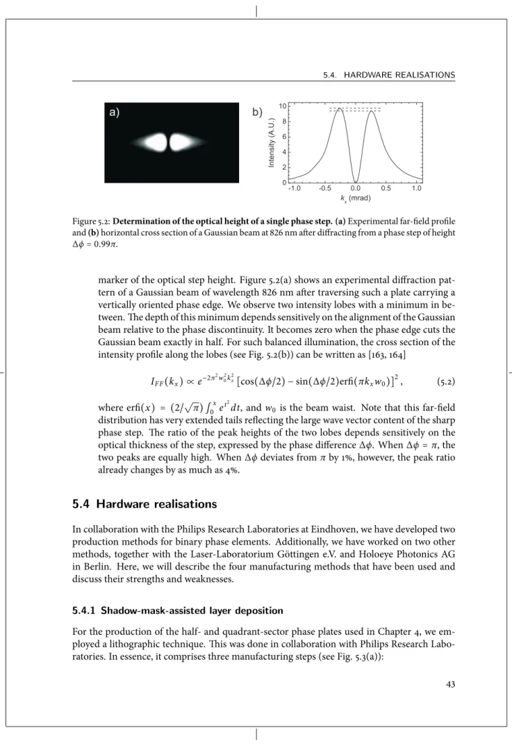
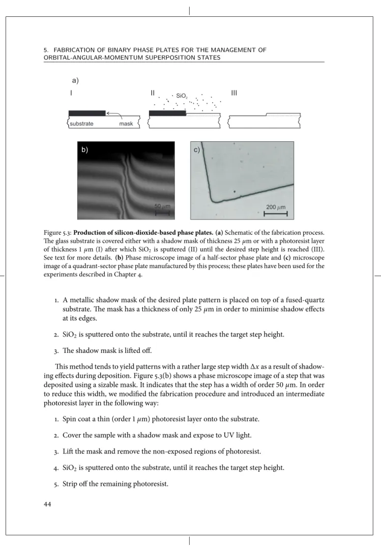
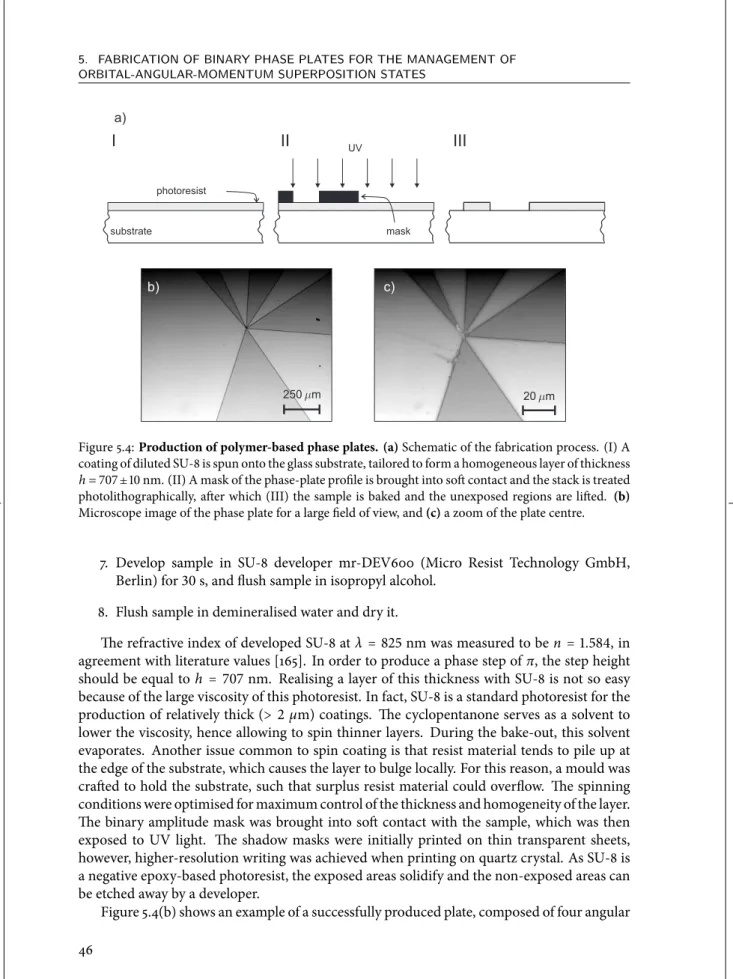
Entangling light in high dimensions
Cover Design: Hanna Troch
Entangling light in high dimensions
PROEFSCHRIFT
ter verkrijging van
de graad van Doctor aan de Universiteit Leiden, op gezag van Rector Magnificus prof. mr. P. F. van der Heijden,
volgens besluit van het College voor Promoties te verdedigen op donderdag 3 februari 2011
klokke 13:45 uur
door
Jan Bardeus Pors
Promotor: Prof. dr. J. P. Woerdman Universiteit Leiden
Co-promotor: Dr. E. R. Eliel Universiteit Leiden
Leden: Dr. S. S. R. Oemrawsingh Universiteit Leiden Dr. M. P. van Exter Universiteit Leiden
Prof. dr. G. W. ’t Hooft Philips Research en Universiteit Leiden Prof. dr. M. W. Beijersbergen Cosine B.V. en Universiteit Leiden Prof. dr. S. M. Barnett University of Strathclyde Glasgow
Dr. A. Aiello Friedrich-Alexander-Universit¨at
Erlangen-N¨urnberg Prof. dr. J. M. van Ruitenbeek Universiteit Leiden
Paranimfen: Maartje E. Zonderland en David J. Beerends
The work reported in this thesis was carried out at the ‘Leids Instituut voor Onderzoek in de Natuurkunde’ (LION) and is part of the research programme of the ‘Stichting voor Fundamenteel Onderzoek der Materie’ (FOM).
An electronic version of this dissertation is available at the Leiden University Repository (https://openaccess.leidenuniv.nl).
Wie zich verwondert, geeft zich rekenschap van een wonder.
Contents
1 Introduction 1
1.1 Quantum entanglement . . . 1
1.2 High-dimensional entanglement . . . 2
1.3 Orbital-angular-momentum states . . . 2
1.4 Dimensionality and information . . . 4
1.5 Orbital-angular-momentum-entangled states as information carriers . . . 5
1.6 Outline . . . 5
2 Characterisation of a spontaneous parametric down-conversion source for spatially-entangled photon pairs 7 2.1 Introduction . . . 7
2.2 Phase matching . . . 8
2.3 Experimental results . . . 10
2.4 Estimate of the number of spatially entangled modes . . . 13
2.5 Conclusions . . . 16
3 Angular phase-plate analysers for measuring the dimensionality of multi-mode fields 17 3.1 Introduction . . . 18
3.2 The Heaviside step phase plate . . . 19
3.3 Detection-state expansion in orbital-angular-momentum eigenmodes . . . 20
3.4 Dimensionality . . . 22
3.5 Measuring the effective dimensionality . . . 24
3.6 Discussion . . . 25
3.7 Conclusions . . . 26
4 Shannon dimensionality of quantum channels and its application to photon entan-glement 29 4.1 Introduction . . . 30
4.2 Shannon dimensionality . . . 30
4.3 Experimental results . . . 31
4.4 Conclusions . . . 35
4.5 Appendix . . . 36
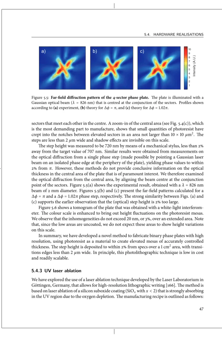
5 Fabrication of binary phase plates for the management of
orbital-angular-momentum superposition states 39
5.1 Introduction . . . 39
5.2 Specifications of hardware binary phase plates . . . 41
5.3 Characterisation of binary phase plates . . . 42
5.4 Hardware realisations . . . 43
5.4.1 Shadow-mask-assisted layer deposition . . . 43
5.4.2 Polymer-based photolithography . . . 45
5.4.3 UV laser ablation . . . 47
5.4.4 Laser-beam lithography . . . 48
5.5 Dynamic devices . . . 51
5.6 Conclusions . . . 53
6 High-dimensional entanglement with orbital-angular-momentum states of light 55 6.1 Introduction . . . 56
6.2 Setting . . . 57
6.3 Binary sector phase plates . . . 58
6.4 Optimisation of binary sector phase plates . . . 60
6.4.1 Single-sector phase plates . . . 60
6.4.2 Multi-sector phase plates . . . 61
6.5 Experimental results . . . 63
6.6 Conclusions . . . 66
6.7 Appendix . . . 67
7 Beyond angular entanglement 69 7.1 Introduction . . . 69
7.2 Setting . . . 69
7.3 Escher phase plates . . . 70
7.4 Relevant parameters and coincidence probability . . . 72
7.5 Experimental results . . . 74
7.6 Conclusions . . . 75
8 Atmospheric turbulence and optical propagation 77 8.1 Introduction . . . 77
8.2 Kolmogorov turbulence . . . 77
8.3 Propagation of light through a turbulent atmosphere . . . 79
8.3.1 Phase structure function . . . 79
8.3.2 Beam propagation . . . 81
8.4 Laboratory implementations of turbulence . . . 83
8.4.1 Random phase screens . . . 84
8.4.2 Turbulence cells . . . 84
8.5 Conclusions . . . 86
CONTENTS
9 Transport of orbital-angular-momentum entanglement through a turbulent
atmo-sphere 87
9.1 Introduction . . . 88
9.2 Experimental setting . . . 88
9.3 Turbulence cell . . . 89
9.4 Results . . . 92
9.5 Discussion . . . 93
9.6 Conclusions . . . 96
9.7 Appendix . . . 96
Bibliography 99
Samenvatting 111
Curriculum Vitæ 113
List of publications 115
Nawoord 117
CHAPTER 1
Introduction
1.1 Quantum entanglement
Quantum entanglement is a most intriguing feature of certain states of composite quantum systems that contain two (or more) distinct objects [1–3]. This fundamental trait of quantum mechanics causes the information about the properties of the objects to be inextricably linked. The entanglement works in such a way that, when a measurement of the properties of one of the objects is performed, the properties of the other object are immediately altered, even when these objects are separated at arbitrary distances.
The consequences of this phenomenon can be so unimaginable that the intuition we de-rive from the everyday world around us is often deceived. First discussed in the early 1930s, it stirred a vigorous debate between Schr¨odinger, Bohr, and Einstein about the fundamen-tal properties of nature, and the acceptability of quantum mechanics as a valid description of natural phenomena. Ever since, entanglement has played a central but controversial role in the development of quantum mechanics, as it clearly exposes the divorce between classical and quantum physics. That is, quantum entanglement refutes the classical idea of a fully de-terministic world, by violating what became known aslocal realism: the classical postulates that (i) objects carry properties prior to and independent of measurements (realism) and (ii) measurement results obtained at one location are independent of actions at another (spacelike-separated) location (locality) cannot be maintained jointly.
In spite of several attempts to bridge this emerging gap between classical and quantum physics, it was John S. Bell who first realised that, if entanglement were to exist, it should give rise to correlations between outcomes of measurements that are stronger than any classical theory allows for [4]. His seminal work of 1964 provided the framework to investigate quantum entanglement experimentally. Another 15 years later, some 50 years after the original dispute, the existence of quantum entanglement was first demonstrated in the laboratory [5, 6]. Since then, a multitude of experiments have corroborated these findings, using entangled states of light, electrons, atoms, molecules, and Bose condensates.
In recent years, the view on quantum entanglement has become more pragmatic, when it was realised that quantum entanglement could have application in information science. In principle, the strong quantum correlations exhibited by entangled systems enable computation
and communication tasks that are beyond reach of classical methods [7]. This perspective has proved fruitful and has resulted in such ideas as quantum computation [7], quantum metrol-ogy [8], quantum imaging [9], and quantum cryptography [10], to name a few. Although technologically still in its infancy, modern research on entangled systems is largely driven by the prospect of such applications, creating a bustling field of research known as quantum in-formation processing.
1.2 High-dimensional entanglement
In this thesis, we will be concerned with entangled states of light. Historically, quantum states of light, i.e.,photons, have played a prominent role in the experimental study of quantum entanglement. For instance, the first Bell tests [5, 6] and first realisations of quantum telepor-tation and quantum cryptographic key distribution were all performed using entangled two-photon states [11]. The vast majority of this work involves the use of the polarisation degrees of freedom of light [11]. Such polarisation-entangled states are appealing from a conceptual point of view, because the two entangled polarisation eigenmodes form an insightful binary system. From an experimental point of view, such states are readily prepared and managed using conventional polarisation optics.
Recently, however, both theoretical and experimental efforts have shifted towards entan-glement inmore than two modes. This generalised form of entanglement is often referred to as high-dimensional entanglement. The motivation for this work stems from the realisation that, with an increasing number of entangled modes, entanglement becomes correspondingly richer. This is, for instance, reflected in stronger violations of various measures of non-locality, which reveal the complexity of high-dimensional Hilbert spaces [12–15]. From an applications perspective, high-dimensional entanglement also has considerable advantage. For example, it carries promise to provide a larger channel capacity [16, 17] and improved security [18, 19] for quantum communication, and simplifies logic-gates architecture [20].
With increasing dimensionality, however, the analysis of entanglement becomes corre-spondingly more complex, both theoretically and experimentally. For a start, it is not straight-forward to define entanglement criteria in high dimensions. For instance, it not easy to distin-guish unambiguously between classical and quantum correlations [12–15], or to quantify en-tanglement for high-dimensional mixed states [21]. Second, the number of operations needed to determine properties of the state (such as entanglement witnesses or separability criteria) typically increases steeply with the number of entangled modes. Experimentally, this implies that a large number of resources tends to be needed to investigate high-dimensional entangle-ment.
Given this situation, it is both interesting and relevant to investigate how much one can learn about high-dimensional entanglement from a limited set of measurements and a small number of resources. Our work aims at exploring this issue.
1.3 Orbital-angular-momentum states
There are several ways to implement high-dimensional two-photon entanglement. One can exploit the temporal [22, 23], frequency [24] or spatial [25–28] properties of the optical field.
1.3. ORBITAL-ANGULAR-MOMENTUM STATES
It is also possible to use combinations of different degrees of freedom, known as hyperentan-glement [29–31].
A promising way to implement high-dimensional entanglement involves the use of the orbital-angular-momentum (OAM) degree of freedom of light [28]. Light beams that carry OAM have a helical wavefront that spirals around the optical axis during propagation [32]. The OAM content of the field is related to the winding numbermof the helicity, and amounts tomħper photon. Unlike thespinangular momentum of light, which is associated with the polarisation and is limited to a value between−ħandħ, theorbitalangular momentum
con-tent of light is unbounded, in the sense that the number of distinguishable OAM modes that have the same propagation axis is, in principle, infinite. The winding numberm, which char-acterises the OAM eigenmodes, can adopt any integer value between−∞and∞. Moreover,
all coaxial OAM modes are mutually orthogonal and they thus span a very high-dimensional Hilbert space.
For the work discussed in this thesis, we follow this approach to high-dimensional entan-glement. In the following, we briefly discuss how OAM-entangled states can be generated and how they can be analysed.
The simplest and most common way to produce entangled photon pairs is through the process of spontaneous parametric down-conversion. In this nonlinear process, a “blue” pump photon is spontaneously converted into two “red” photons, while conserving energy, momen-tum and angular momenmomen-tum. Typically, the generated photon pair is entangled in many de-grees of freedom, like polarisation, frequency and transverse momentum. We focus on the latter aspect, or more specifically on the angular transverse momentum, and configure our system such that it produces a very large number of entangled OAM modes [33–35]. The cor-relations between the two photons of a pair are tuned such that they have opposite OAM. The number of entangled modes is typically of the order of 60.
As mentioned above, full state determination of high-dimensionally entangled states is not straightforward. Various experimental techniques have been devised to sort the modes of an OAM superposition state by their mode number, some of which have been applied to the quan-tum regime [36–39]. However, to assess or witness entanglement, this generally does not suf-fice, as one has to measure observables in various unbiased state bases. In the first experiments on OAM entanglement, which probed a 3-dimensional space, this issue was tackled by clev-erly manipulating the OAM analysers [40, 41]. This approach was improved on by using either holographic [42] or interferometric means [43], providing the possibility to perform full state tomography. However, scalability of these methods to systems of larger dimensionality than 3 has not been demonstrated, and may not be realistic. An interesting alternative exploits a com-bination of the polarisation and OAM mode structure of the field [29]. Recently, OAM and its conjugate variable, the transverse angular position, have been shown to exhibit correlations that are a signature of entanglement [44]. Also in the domain of continuous-variable states, quadrature entanglement has been demonstrated between low-order OAM modes [45, 46]. Obviously, there are many approaches possible, and the challenge is to devise an approach that is easily implementable, reliable and yields as much information as possible.
The approach we follow is to investigate high-dimensional OAM entanglement by making use of onlytwostate analysers [47]. Pivotal to the approach is the use of state projecting ele-ments, consisting of an optical phase plate that is lens-coupled to a single-mode fiber. These phase plate are diffractive optical elements, the optical thickness of which has an angular
ation. They can be used to imprint an azimuthally dependent phase profile onto a beam, and in this way we can control and modify the OAM content. In view of the fact that the pho-tons of a pair have opposite OAM, we employ complementary phase plates in the two beam lines of our down-conversion setup; that is, the two phase plates are each other’s conjugate. Furthermore, the phase plates can be rotated around their central axis. In this way, the OAM projection states can be varied, which allows the analysers to probe a Hilbert space of large dimensionality. The exact size of this Hilbert space is determined the complexity of the spatial pattern of the phase plates.
1.4 Dimensionality and information
Already in the early days, Schr¨odinger made a notable observation on entanglement, when he stated that “...knowledge of the individual systems can decline to the scantiest, even to zero, while that of the combined system remains continually maximum. The best possible knowl-edge of a whole doesnotinclude the best possible knowledge of its parts” [2]. In other words, he established a connection between entanglement and the notion of information. The strik-ing trait of quantum entanglement that full information about the composite system is not identical to full information about the subsystems it consists of, is contradictory to anything we know from classical physics. Or, as Schr¨odinger concludes: “this is what keeps coming back to haunt us”.
The information content of a general state can be quantified in terms of the entropies of the composite system and the individual subsystems. Probably, the most commonly used measure of this sort is the Von Neumann entropy, defined asS= −Trρlogρ, withρa normalised density operator [7]. It is equally valid, however, to characterise the state is terms of the purity of the combined system and the subsystems, which is defined asP=Tr(ρ2).*Note that the purity of ρyields the average of its eigenvalue probabilities, and in general we will have 0≤Tr(ρ2) ≤1. Let our two-photon state of interest be described by the normalised density operatorρAB, and its subsystems byρA = TrB(ρAB)andρB = TrA(ρAB). In this thesis, we will
predomi-nantly focus our attention on pure states. In this case, we have
P=TrAB(ρ2AB) =1, and K=
1 TrA(ρ2A)
=
1 TrB(ρ2B)
. (1.1)
The fact thatP = 1 reflects thatρABhas a single eigenvalue. The numberK, formally a par-ticipation ratio and known as the Schmidt number, is given by the inverse of the purity of the subsystems. A very interesting property of this quantity is that it is a measure of the num-ber of entangled modes of the system: as the purity of the subsystems represents the average probability of their eigenvalues,Kyields the effective dimensionality of the state [49, 50].
The quantities discussed so far, however, provide information about the properties of the generatedquantum state. In an actual quantum experiment, one analyses the state with a detec-tion apparatus that has properties of itself. In other words, the detecdetec-tion device determineshow muchone can learn about the system. For instance, a limited detection efficiency, as present
*Note that the Von Neumann entropy and the purity are related to each other and emerge as the first and second order realisations of the generalised Tsallis entropies, respectively [48].
1.5. ORBITAL-ANGULAR-MOMENTUM-ENTANGLED STATES AS INFORMATION CARRIERS
in practically all experiments, sets a limit to the accuracy and reliability of the measurement of system properties.
In particular, the detection apparatus may set a limit to the number of modes of the system that one can distinguish,i.e., an experimental outcome on the number of entangled modes may be mostly determined by the detection system, rather than by the source. It is therefore extremely useful to develop a quantifier for the dimensionalityas measured in an experiment [51, 52]. This is one of the main issues addressed in this thesis and we will introduce what we refer to as the Shannon dimensionality of measured entanglement.
1.5 Orbital-angular-momentum-entangled states as information
car-riers
Photons being a natural candidate to transmit information, quantum communication is one of the most promising applications of two-photon entanglement. In 1992, Ekert showed how entanglement could add to the security of quantum communication, as compared to single-photon protocols [10]. Since the proof-of principles demonstrations [11], impressive techno-logical advance has been made. Nowadays, secure communication distances range up to hun-dreds of kilometres, both for fiber-based [53–55] and free-space [56–58] transmission links, and even a satellite quantum connection may be within reach [59]. Improving on signal band-widths and the suppression of losses, however, remains a challenging issue. All this work was done using 2-dimensional entanglement.
Recently, it was realised that quantum-communication protocols could benefit signifi-cantly from entanglement in dimensions higher than 2. This extension provides the potential of an increased information capacity [16, 17] and an enhanced security against eavesdropping [18, 19]. Some of these principles have already been realised in the laboratory, implementing the high dimensionality by means of energy-time or OAM entanglement [23, 60–62].
This raises the question whether OAM entanglement could be implemented for quantum communication in a real-world setting. Successful implementation requires that the OAM en-tanglement can be transported over a sufficiently long distance, via a fiber-based or free-space link. The performance of such a quantum channel, however, is an open issue. Several studies have addressed this aspect for the case of free-space distribution, but there is no unanimity on exactly how robust OAM entanglement is [63–71]. On the one hand, it was suggested that the topological charge of light is a resilient quantity, supporting its use as an information car-rier in free-space communication. On the other hand, having the information encoded in the wavefront structure of the field, OAM entanglement may be vulnerable to refractive-index fluctuations that arise due to atmospheric turbulence. In the final two chapters of this thesis, we explore this issue experimentally.
1.6 Outline
This thesis is organised as follows. In Chapter 2, we discuss how we create OAM-entangled photon pairs by means of parametric down-conversion, and we experimentally characterise the emission of our source. In Chapter 3, we introduce our angular state analysers, and quantify the dimensionality of the Hilbert space they probe. Chapter 4 unites the preceding two
ters and demonstrates how to extract high-dimensional OAM entanglement from a down-conversion source by means of such analysers. Furthermore, this Chapter introduces the con-cept of the Shannon dimensionality of measured entanglement, and experimentally we achieve D=3 and 6. In order to realise OAM entanglement of increasing dimensionality, phase plates with a growing amount of complexity are required. Various fabrication methods of such phase plates are discussed in Chapter 5. In Chapter 6, we extend on the ideas from Chapter 4 and demonstrate how to extract genuinely high-dimensional OAM entanglement. In Chapter 7, we go beyond the use of OAM-entangled states, and take a first step towards incorporation of both the angular and the radial degree of freedom. We discuss some of the consequences of this generalisation and present an experimental demonstration. In the final two Chapters, we study whether two-photon OAM entanglement could be useful for free-space quantum com-munication. Chapter 8 presents an overview of the theory of optical propagation through the atmosphere, and describes the experimental techniques we have developed to generate realis-tic atmospheric turbulence in a laboratory environment. In Chapter 9, we present the results of an experimental study of the robustness of OAM entanglement when subject to atmospheric turbulence.
CHAPTER 2
Characterisation of a spontaneous parametric
down-conversion source for spatially-entangled photon
pairs
2.1 Introduction
Spontaneous parametric down-conversion (SPDC), in the older literature frequently referred to as parametric fluorescence or parametric scattering [72–74], is a second-order nonlinear op-tical process in which a high-frequency photon spontaneously splits in two lower-frequency photons, such that energy is conserved. It is thereby the inverse process of the more widely known up-conversion processes of second-harmonic generation (SHG) and sum-frequency generation (SFG), where two low-frequency beams are nonlinearly mixed to produce one high-frequency component [75, 76].
The process of SPDC has found common application in various fields of research. In the past, it has been used as a tool to measure the second-order nonlinear optical susceptibility tensor for a variety of materials [77–79]. An advantage of this method over more common methods based on SHG and SFG [80], lies in the fact that in SPDC the conversion efficiency is independent of the pump power, hence obviating the need for detailed knowledge of the pump beam’s characteristics. SPDC is also the initiating process in optical parametric oscillators, as it generates the seed photons from which the coherent output builds up via parametric amplifi-cation [74, 81]. Owing to their large frequency tuning range, parametric oscillators are popular sources of tunable, narrowband light in a variety of fields, ranging from coherent anti-Stokes Raman spectroscopy [82] to continuous-variable quantum optics [83]. In recent years, SPDC has made its mark on the fields of quantum optics and quantum information, as a source of quantum states of light. In particular, it has become a standard instrument for the production of entangled photons [84–86], paving the way for such applications as quantum cryptography, quantum teleportation, quantum imaging, etc. [9, 11]. To date, SPDC remains an unparalleled source of entangled photon pairs in terms of brightness, reliability, and universality.
For the experimental work presented in this thesis, we exploit the process of SPDC for the creation of orbital-angular-momentum (OAM) entangled photon pairs. The efficiency of the
ks Dk z
ki
^ z kp
z
Figure 2.1:Representation of the pump, signal, and idler wave vectors in SPDC.The down-converted signal and idler wave vectorsks andki point away from the pump wave vectorkpin such a way that
transverse momentum is conserved. The longitudinal mismatch is denoted as ∆kz.
conversion process depends, amongst others, strongly on the wave-vector mismatch ∆k be-tween the pump and down-converted photons travelling through the nonlinear medium. This sensitivity on the mismatch sets limits to the spatial distribution in which the down-converted light is emitted. Consequently, when studying spatial (quantum) correlations between the pho-tons in a pair, it is important to have a full understanding of the spatial structure of the SPDC source, and the dependence thereof on phase matching.
In the present Chapter, we present the results of an experimental characterisation of our SPDC source. We study the spatial structure of the down-converted light by imaging the far field of the light emitted from the nonlinear crystal and investigate the dependence of the emis-sion on phase matching. The experimental data are used to estimate the number of entangled modes emitted by our source, characterised by the Schmidt number [50, 87]. This number serves as a benchmark for the work in the ensuing Chapters of this thesis, substantiating some useful assumptions we make regarding the spatial structure of the entanglement.
2.2 Phase matching
The process of SPDC does not exchange energy with the nonlinear crystal, and, consequently, the energy of a pump photonħωpreappears as the sum of the energies of the two generated photons:
ωp=ωs+ωi. (2.1)
Here,ωsandωirefer to the frequencies of the generated photons, traditionally named signal (s) for the high-frequency photon and idler (i) for the low-frequency partner.
In the limit that the transverse cross section of the nonlinear crystal is much larger than that of the pump beam, the setup is invariant to translations in the plane of the crystal. Con-sequently, the transverse component of the wave vector has to be conserved. This implies that the signal and idler photons in a pair have equal but opposite transverse wave vectors. Because of the finite length of the crystal, the longitudinal component of the wave vector does not need to be conserved; the ensuing wave-vector mismatch between the pump, idler, and signal waves is given by (see Fig. 2.1)
∆k=∆kz =kp,z−ks,z−ki,z. (2.2) Here, kj = 2πnj/λj, withnjthe (wavelength-dependent) refractive index of the nonlinear medium andλjthe wavelength of the light.
The efficiency of any nonlinear optical process depends strongly on this wave-vector mis-match. The emission is brightest if the various fields are coherent over the full length of the
2.2. PHASE MATCHING
crystal. For that reason, nonlinear optical processes are preferably operated under phase-matched conditions,viz., ∆k≃0.
Dispersion in the nonlinear material between pump, signal, and idler waves hereby plays an inhibiting role and should be eliminated. This can be achieved with the use of birefringent nonlinear crystals. In such crystals perfect phase matching can be attained by appropriately orienting the crystal axes, and the wave vectors and polarization vectors of the input fields. However, it is often the case that the strongest nonlinearities cannot be addressed in this man-ner. Consequently, considerable effort has been devoted to develop materials that combine perfect phase matching with a strong nonlinear response, resulting in a multitude of quasi-phase-matched and periodically-poled materials [88, 89].
In up-conversion processes such as SHG and SFG, the concept of phase matching has a clear experimental significance: it simply determines the net power of the up-converted beam. This is due to the fact that the two fixed input waves impose quite a stringent condition on the frequency and directionality of the generated harmonic. When perfect phase matching is not met, the emitted radiation is much weaker and modulates rapidly as a function of the phase mismatch. This behaviour was first reported by Makeret al., who investigated SHG from a crystalline quartz sample [90]. Although quartz does not allow for perfect phase matching, they observed a weak second-harmonic signal that varied in power with the orientation of the crystal,i.e., with ∆k. Nowadays, this modulation goes by the name of “Maker fringes” [91, 92]. In SPDC, the system has more freedom to obey the phase-matching condition, and a change of the crystal orientation does not necessarily lead to an increase or decrease in the radiated power. Rather, it may result in a directional and/or frequency redistribution of the emitted radiation, since Eqs. (2.1) and (2.2) together allow for a certain freedom in the fre-quencies and directionalities of the generated photons. This flexibility lies at the heart of the wide tuning range of parametric oscillators. Nevertheless, power variations equivalent to those encountered in SHG and SFG appear when the output power is measured within a narrow spectral bandwidth and within a well-defined range of wave vectors, that is, if one is selective regarding the frequency-mode and spatial-mode structure of the SPDC light.
Let us study the spatial structure of the SPDC emission in closer detail. In a plane-wave description, the down-converted field emanating from a non-linear crystal of lengthLis of the general form
E∝ ∫
L
0
ei∆kzzd z ∝
sin(12∆kzL)
1 2∆kzL
L. (2.3)
This function is strongly peaked around ∆kz=0, corresponding to perfect phase matching.
polarization entangled photon pairs [86]. In our pursuit to create OAM-entangled photons, on the contrary, we have chosen to use Type-I phase matching. In this configuration, signal and idler photons have the same polarization and emerge in a single cone coaxial with the pump beam axis. The aperture of the cone can be widened or shrunk by tuning the phase-matching. Of particular interest is the situation that the cone is contracted to the point that the emission is beam-like. This relieves the need of apertures and the accompanying truncation of spatial modes.
Equation (2.3) shows that the strength of the generated field is proportional to the crystal lengthL, while the width of the phase-matched cone is inversely proportional toL. Away from perfect phase matching, emission is fully inhibited whenever ∆kzLequals a multiple of 2π, but revives weakly in between these nodes. These fringes constitute the SPDC analogy of Maker’s observation; they have a spatial character and appear as rings around the perfectly phase-matched emission cone, somewhat reminiscent of an Airy diffraction pattern.
In the following Section, we will present experimental data of the spatial structure of the SPDC emission from a Type-I source.
2.3 Experimental results
In our experiment, we use a BBO crystal (β-barium borate,β-BaB2O4) that allows for Type-I phase matching by angle tuning of the crystal. Figure 2.2 shows a diagram of our experimental setup. The crystal of length 1 mm is pumped by a weakly focused (waistw0 =250 µm) Kr+ laser beam of 100 mW power at a wavelength of λ = 413 nm. The pump beam is polarised along the extraordinary crystal axis, whereas the signal and idler beams are polarised along the ordinary axis. The phase mismatch can then be written as
∆kz=2π[
ne(λp, Θ)
λp
−
no(λi)
λi
−
no(λs)
λs
], (2.4)
where the subscripts(o,e)denote the ordinary and extraordinary crystal axes, respectively.
The extraordinary refractive indexne depends on the tuning angle Θ between the direction of propagation and the optical axis of the crystal. The effective nonlinearity of BBO cut for Type-I collinear phase matching (Θ= 28.3○) equalsdeff =1.9×10⁻¹²m/V [93]. Given the 1
mm crystal length, the total yield of the resulting down-converted light is only of the order of 104photon pairs per second per spatial mode per nm bandwidth. This feeble signal must
be filtered from the 100 mW pump beam (≃ 1017photons per second), which is achieved by
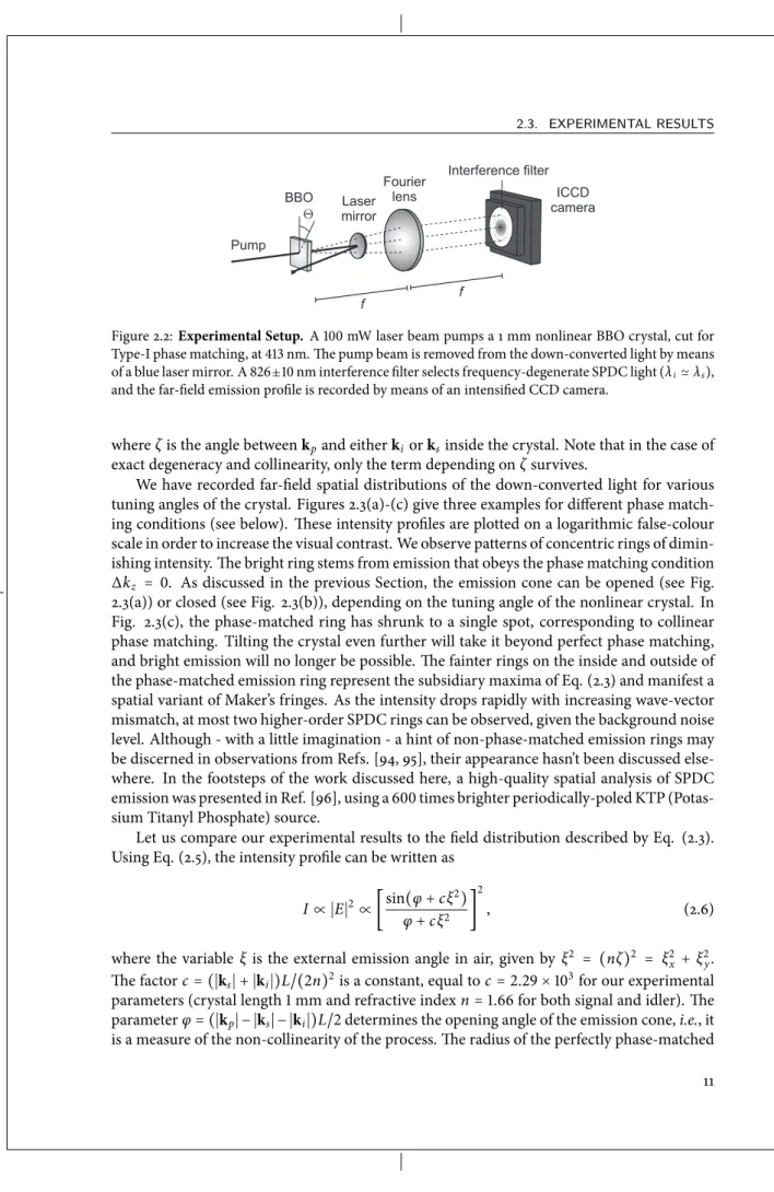
means of a blue laser mirror that reflects the pump beam. Additionally, an interference filter, centred around 826 nm with a 20 nm width, suppresses residual stray (pump) light and ensures that we detect only degenerate photon pairs withλi ≃λs. We use an intensified CCD camera (Princeton PI-MAX) that is positioned in the Fourier plane of the crystal to detect the SPDC light. This far-field configuration enables us to characterise the angular emission profile of the degenerate down-converted light.
We will work close to the point where ∆kz =0 and, furthermore, close to collinearity where signal and idler point in the same direction as the pump beam. Becauseλi ≃ λs ≃2λp, the phase mismatch can be approximated by
2.3. EXPERIMENTAL RESULTS
Pump
Laser mirror BBO
f f
Fourier
lens ICCD
camera Interference filter
Q
Figure 2.2:Experimental Setup.A 100 mW laser beam pumps a 1 mm nonlinear BBO crystal, cut for Type-I phase matching, at 413 nm. The pump beam is removed from the down-converted light by means of a blue laser mirror. A 826±10 nm interference filter selects frequency-degenerate SPDC light (λi≃λs),
and the far-field emission profile is recorded by means of an intensified CCD camera.
whereζis the angle betweenkpand eitherkiorksinside the crystal. Note that in the case of exact degeneracy and collinearity, only the term depending onζsurvives.
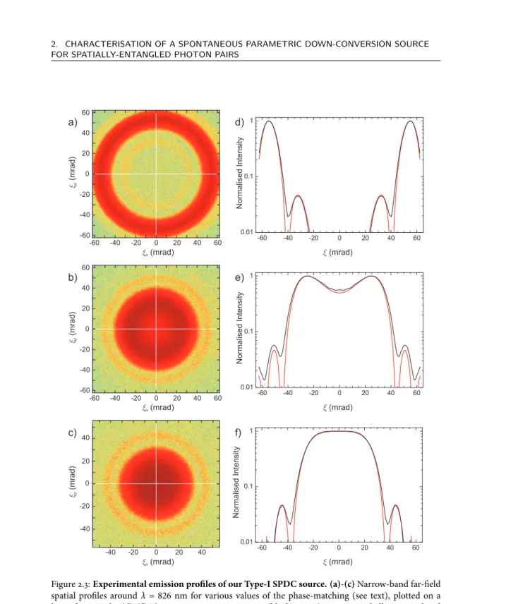
We have recorded far-field spatial distributions of the down-converted light for various tuning angles of the crystal. Figures 2.3(a)-(c) give three examples for different phase match-ing conditions (see below). These intensity profiles are plotted on a logarithmic false-colour scale in order to increase the visual contrast. We observe patterns of concentric rings of dimin-ishing intensity. The bright ring stems from emission that obeys the phase matching condition ∆kz = 0. As discussed in the previous Section, the emission cone can be opened (see Fig.
2.3(a)) or closed (see Fig. 2.3(b)), depending on the tuning angle of the nonlinear crystal. In Fig. 2.3(c), the phase-matched ring has shrunk to a single spot, corresponding to collinear phase matching. Tilting the crystal even further will take it beyond perfect phase matching, and bright emission will no longer be possible. The fainter rings on the inside and outside of the phase-matched emission ring represent the subsidiary maxima of Eq. (2.3) and manifest a spatial variant of Maker’s fringes. As the intensity drops rapidly with increasing wave-vector mismatch, at most two higher-order SPDC rings can be observed, given the background noise level. Although - with a little imagination - a hint of non-phase-matched emission rings may be discerned in observations from Refs. [94, 95], their appearance hasn’t been discussed else-where. In the footsteps of the work discussed here, a high-quality spatial analysis of SPDC emission was presented in Ref. [96], using a 600 times brighter periodically-poled KTP (Potas-sium Titanyl Phosphate) source.
Let us compare our experimental results to the field distribution described by Eq. (2.3). Using Eq. (2.5), the intensity profile can be written as
I∝ ∣E∣2∝ [
sin(φ+c ξ2)
φ+c ξ2 ] 2
, (2.6)
xx(mrad)
0 20 40
-40 -20 60
-60 xy (mrad) 0
-40 -20 20 40
-60 60
xx(mrad)
0 20 40
-40 -20 60
-60 xy (mrad) 0
-40 -20 20 40
-60 60
xx(mrad)
0 20 40
-40 -20 xy
(mrad) 0
-40 -20 20 40
a) d)
b) e)
c) f)
x(mrad) x(mrad) x(mrad)
2.4. ESTIMATE OF THE NUMBER OF SPATIALLY ENTANGLED MODES
SPDC ring in the Fourier plane is given byξR= √
−φ/c. The phase-matched cone is open for
φ <0, with collinearity occurring atφ= 0. Forφ> 0 perfect phase matching is no longer possible.
Figures 2.3(d)-(f) show the cross sections (solid curves) of Figs. 2.3(a)-(c), respectively. These cross sections, obtained after careful determination of the profile centres, were az-imuthally averaged and normalized to maximum intensity. The dashed curves represent the theoretical prescription from Eq. (2.6), where only the “non-collinearity”φwas left as a fitting parameter. From these fits, we foundφ = −6.90 rad andφ= −1.40 rad for Fig. 2.3(d) and 2.3(e), respectively. For Fig. 2.3(f) we obtainedφ = −0.05 rad, in correspondence with the statement thatφ→0 at collinearity. Similar results were obtained when leavingcas a second fitting parameter.
2.4 Estimate of the number of spatially entangled modes
The intensity measurements in Fig. 2.3 of the parametric fluorescence from the nonlinear crystal are in itself classical. Between the signal and idler photons, however, exist spatial cor-relations that are essentially of quantum nature. This has been confirmed and exploited in numerous experiments [40, 44, 47, 97], and here, we will adopt a quantum description of the emission without further justification.
As argued in Section 2.2, signal and idler photons in a pair have equal but opposite trans-verse momenta. Both signal and idler photons are individually in a superposition of spatial modes, in such a way that their composite state is pure and entangled. In view of our work in the coming Chapters, we will write this entangled state in a cylindrical basis, namely [33, 34],
∣Ψ⟩ = ∑
m,p
cm p∣m,p⟩A∣ −m,p⟩B. (2.7)
Here,∣m,p⟩A(∣m,p⟩B) represents a signal (idler) spatial mode containing one photon, with
p≥0 a radial andm= −∞, . . . ,∞an azimuthal integer mode index. The entangled state of
Eq. (2.7) is represented in its diagonalised Schmidt decomposition, meaning that it is written as a sum over biorthogonal product states (and the modes of photonsAandBthus carry the same indicesmandp) [98]. The complex expansion coefficientscm pobey the normalization requirement∑m,p∣cm p∣2=1.
In general, it is not a trivial task to find the mode functions fm,p(r) = ⟨r∣m,p⟩for
down-conversion systems as those described in Section 2.2. Approaches to do so can be found in Refs. [33, 87, 99]. Due to the cylindrical symmetry in Type-I phase matching, however, the azimuthal content is readily obtained; the eigenmodes of rotation around the symmetry axis are of the formei m θ, and thus fm,p(r) = fm,p(r)ei m θ, withθthe azimuthal angle. Modes
of this form are also eigenmodes of the OAM operator ˆLz = −i ∂/∂θ[100], and∣m,p⟩thus
represents a spatial mode containing one photon with OAMmħ. Note that conservation of OAM (mA= −mB) was already incorporated in Eq. (2.7).
Figure 2.4:Azimuthal probability distribution of the generated state.Spiral contentPm = ∑p∣cm p∣2
of the Schmidt decomposition (see Eq. (2.7)), calculated for our system. We assumed collinear phase matching and used the experimental parameters as given in Section 2.3.
gives the OAM probability distributionPm, obtained by summing over the radial part,
Pm= ∑
p
∣cm p∣2. (2.8)
Figure 2.4 shows the spiral bandwidth of our source, calculated for collinear phase matching and the experimental values for the pump beam waistw0and the crystal lengthLmentioned in Section 2.3 [35]. We observe a broad spectrum that is symmetric aroundm=0, which is a consequence of the fact that our Gaussian pump hasm=0. The histogram has a considerable width with long tails extending to highmnumbers. Obviously, however, the modes in the superposition carry unequal weights.
In principle, the number of entangled modes in Eq. (2.7) can be infinite. However, it is natural to take the relative weight of the modes into account and to define aneffectivenumber of entangled modes. This is done by the so-called Schmidt number, given by [50, 87]
K= 1
∑m,p∣cm p∣4
, (2.9)
For the case that one is only interested in the azimuthalm-content (i.e., the spiral bandwidth) of the state, it can be derived that [34]
Kaz= 1
∑mPm2
≃2 √
K. (2.10)
The Schmidt number is commonly used as a meaningful quantifier of (high-dimensional) en-tanglement [87].
In principle, if one manages to construct the Schmidt basis{∣m,p⟩}, the Schmidt
2.4. ESTIMATE OF THE NUMBER OF SPATIALLY ENTANGLED MODES
presented two independent methods to measure the Schmidt number experimentally. In the following, we use these methods to estimate the Schmidt number for our experimental con-figuration.
In Ref. [87], Law and Eberly provided an approximation in terms of the ratio of the far-field beam widthsσpu m pandσS P D Cof the pump and SPDC emission, respectively,
K≃
1 4(
σpu m p
σS P D C + σS P D C
σpu m p) 2
, (2.11)
whereσpu m p = 2/w0 and σS P D C = √
4kp/L. Implicit to this result are the assumption of
collinear phase matching and the approximation of Eq. (2.6) by a Gaussian of widthσS P D C. Equation (2.11) constitutes in fact a lower limit toK[87]. Filling in the relevant experimental numbers for the pump beam waist, wave number, and crystal length, we arrive atK=395 (and Kaz = 40). Evidently, the widthsσpu m p andσS P D Ccan also be estimated experimentally. In Fig. 2.5 we reproduced the far-field intensity profile of the source for nearly collinear phase-matching. The inset shows the Gaussian profile of the pump beam in the same plane.* The
scale of the inset is magnified by a factor of five compared to the main graph. We observe that the pump beam is much more compact than the generated SPDC light. We made a rough estimate of the angular widths by simply taking the full width at half maximum and arrived atσS P D C=48 mrad andσpu m p =1.2 mrad. Equation (2.11) thus yieldsK=385 (Kaz =39), in
good agreement with the calculation presented above. As stated earlier, this result based on Eq. (2.11) constitutes a lower boundary to the Schmidt number.
Recently, a more accurate method to measure the Schmidt number was demonstrated in Ref. [101]. Using concepts from classical coherence theory, this method takes into account the detailed spatial structure of the two-photon field. It yields the Schmidt number in terms of the spatial degree of coherence of field,
K≃ 1 λ2
[∫ IN F(r)dr]2 ∫ I2N F(r)dr
[∫ IF F(ξ)dξ]2 ∫ I2F F(ξ)dξ
(2.12)
whereIN F(r)andIF F(ξ)are the spatial intensity profiles of the down-converted light
mea-sured in the near field and far field of the nonlinear crystal, respectively. In the near field, the SPDC profile simply adopts the Gaussian profile of the pump beam (see inset Fig. 2.5). In the far field, the profile shows the concentric structure as presented in Fig. 2.5. Based on the theoretical descriptions for the near field and far field (see Eq. (2.6)), we calculate the Schmidt number to beK=930. Using the experimental data from Fig. 2.5, we obtain an experimental
value ofK=850, probably being a slight underestimate due to the noise floor of the
measure-ment.
In summary, the calculated Schmidt number based on Eq. (2.12) is confirmed by our ex-periment. Moreover, this result is consistent with the lower bound according to Eq. (2.11).
*
xx(mrad) xy
(mrad)
0 20 40
-40 -20 0
-40 -20 20 40
5x
Figure 2.5:Experimental determination of the Schmidt number.Narrow-band far-field intensity pro-file of the SPDC light for collinear phase matching, reprinted from Fig. 2.3(c). The circle indicates the full-width-at-half-maximum intensity level of the central spot. Inset: size of the Gaussian pump beam in the same plane, plotted with five times magnification for comparison. A rough estimate of the Schmidt number is obtained by taking the ratios of the two beam sizes (see Eq. (2.11)), yieldingK=385. A more
careful analysis based on Eq. (2.12) yieldsK=850.
2.5 Conclusions
We have characterised the parametric fluorescence from a Type-I SPDC source, which we will employ in the coming Chapters to create OAM-entangled photon pairs. The emission profiles were spatially analysed, and the influence of phase matching on the emission cone aperture was studied. Apart from dominant phase-matched emission, we observed secondary non-phase-matched emission rings, which are a spatial analogy of the well-known Maker fringes exhibited in second-harmonic generation and sum-frequency generation.
CHAPTER 3
Angular phase-plate analysers for measuring the
dimensionality of multi-mode fields
Analysers comprised of an angular phase plate and a single-mode fiber have recently been introduced to study the angular profile of optical fields. Here, we quantify the number of degrees of freedom, or modes, that such an analyser can resolve. Its performance is described by means of an angular coherence function and we introduce a novel dimensionality that gives theeffectivenumber of modes that a given analyser can probe. This quantity can, as we show experimentally, easily be retrieved from a dual analyser setup.
3.1 Introduction
During the last fifteen years, impressive advance has been made on wavefront control of optical fields. A striking example of this progress is found in the technique of adaptive optics imag-ing [102], where a spatial light modulator [103] or micro-mirror array [104] performs dynamic wavefront corrections on an impinging field. Currently, several devices, known as diffractive optical elements, are available to manipulate or analyse the azimuthal phase profile of a beam. Among these are angular phase plates [105–107] and amplitude holograms [38, 108, 109] or phase holograms [110, 111]. An angular phase plate is a transmissive (or reflective) plate whose optical thickness has a purely angular variation, hence imprinting into a field an azimuthally dependent phase retardation. When the angular variation of the optical thickness is superim-posed with a spatial carrier frequency, we deal with a phase hologram.
In recent years, the azimuthal phase dependence of optical fields has drawn much atten-tion, both from a fundamental and applied perspective. It was realised that the azimuthal phase profile of a paraxial electromagnetic field can be identified with the orbital angular mo-mentum carried by that field (mħper photon, withma discrete index) [32, 37]. Nowadays, orbital-angular-momentum states find their application in optical tweezers [112, 113], in cold-atom physics [114], and in the manipulation of Bose-Einstein condensates [115, 116], where they are utilised to rotate samples.
Orbital-angular-momentum states, of which there are infinitely many, were also addressed in twin-photon experiments [40, 47], motivated by the advantages that quantum entanglement in a high-dimensional mode space might provide for quantum-information science [12]. The experiments employed similar field analysers composed of a diffractive optical element, a fo-cussing lens and a single-mode fiber that is coupled to a photodetector. The important aspect introduced in Ref. [47] was to rotate the diffractive element around the propagation axis of the field. In the current article, we will investigate this class of field analysers, in particular regarding their capability to measure the dimensionality of an incident field by rotating the diffractive element.
As mentioned above, the angular phase operation performed on the field can be realised with either an amplitude or phase hologram [40] or an angular phase plate [47]. Although these devices are in many respects very similar, the use of a phase hologram in a field analyser as described above has a drawback because of the beam deflection that is inherent to its operation; when the hologram is to be rotated, it would imply that the fiber must be translated, which greatly complicates a practical implementation. In contrast, phase plates are purely zero-order devices and hence do not suffer from this disadvantage. We will therefore, without loss of generality, assume that the diffractive phase object be a phase plate.
3.2. THE HEAVISIDE STEP PHASE PLATE
The detection state of the analyser as a whole is given by the fiber’s Gaussian mode com-bined with the angular phase plate’s operation. This detection state can be expanded in the orbital-angular-momentum eigenmodes of the field so as to reveal its modal content, with expansion coefficients carrying both amplitude and phase. The amplitudes of these complex coefficients are fixed by the physical profile of the phase object; they are ‘engraved’ in the plate. The phase components, in contrast, depend on the orientation angle of the device. The anal-yser’s detection state can be readily customised by designing the appropriate phase plate. For instance, pure orbital-angular-momentum states (integerm) can be selected using so-called spiral phase plates of integer order [105]. This kind of plate acts as a pure ladder operator in orbital-angular-momentum space and increases (or decreases) the orbital angular momentum of the field by an integer multiple ofħper photon. Field analysers equipped with these plates constitute a special class; their expansion in field eigenmodes contains merely one term, and their operation is therefore invariant under rotation of the plate. It was in fact this kind of transformation that was exploited in Ref. [40] (be it by using a fork-shaped phase hologram, rather than a spiral phase plate). The detection state of a general analyser, however, is typically a superposition of numerous, if not infinitely many orbital-angular-momentum eigenmodes (as, for example, for thenon-integer spiral phase plate used in Ref. [47]). In that case, the phases of the various modes will evolve each in their individual way when the plate’s orienta-tion angle is varied. As a consequence, the detecorienta-tion state alters as the phase plate is rotated and the analyser thus scans a potentially high-dimensional mode space.
In this article, we aim to gain a deeper understanding of this behaviour. In particular we address the question how to quantify the number of spatial modes, or dimensionality, that such a field analyser can resolve. In order to do so, we first represent the single-mode analyser by a mutual coherence function and derive an expansion in orbital-angular-momentum eigen-modes. We then discuss the commonly usedfidelitydimensionDfid, which counts thetotal number of modes that can be observed by this type of field analysers [117]. Subsequently, we introduce a novel measure,Deff, that gives theeffectivenumber of angular degrees of freedom that can be resolved. It can be interpreted as the number of information channels available, be it in a non-trivial way. The effective dimensionality is, unlike the fidelity dimension, indepen-dent of experimental conditions. We show that this number can straightforwardly be retrieved from a dual analyser setup and we present experimental data that confirm this.
3.2 The Heaviside step phase plate
To illustrate our general theory, we will apply our findings at several moments in this paper to a Heaviside-step-phase-plateanalyser [118, 119]. We therefore first introduce this specific angular phase-plate analyser.
A Heaviside step phase plate is a transmissive (or reflective) plate having an arc sector whose optical thickness is half a wavelength greater than the remainder of the plate (see Fig. 3.1(a)). The part of the field that crosses this arc sector thus flips sign. The length of the arc section producing theπphase shift is given by the parameter Θ. The plate’s transmission function can simply be written as:
HereH(x)is the Heaviside step function,θis the azimuthal coordinate andαis the orientation angle of the phase plate. The anglesθandαare both measured from the positive direction of a reference axis and are periodic in 2π. A special case is given by Θ = π, in which case the plate consists of two equal halves of phase differenceπ. The corresponding phase operation connected to such a plate is the well-known Hilbert transformation [120].
Assembling an angular phase plate, a coupling lens, a single-mode fiber, and a photode-tector leads to our field analyser. The phase plate and single-mode fiber are placed in their mutual far field, at a focal distance f on either side of the incoupling lens. An illustration of an analyser equipped with a Heaviside plate of arc sector Θ=πis shown in Fig. 3.1(b).
b)
angular phase plate
lenssingle-mode fiber photodetector
f f
a Q
q
a)
Figure 3.1: Angular-phase-plate analyser. (a)Heaviside step phase plate with arc sector Θ producing a phase shiftπwith respect to the remainder of the plate. The plate orientation is denoted byα, andθis the azimuthal coordinate.(b)Angular phase-plate analyser with Heaviside step phase plate having Θ=π.
The impinging field diffracts from the angular phase plate and is coupled to a single-mode fiber by a lens of focal lengthf. The phase plate can be rotated.
3.3 Detection-state expansion in orbital-angular-momentum
eigen-modes
We consider a monochromatic paraxial field of wavelengthλ=2π/k, propagating along the
z-axis of an optical system. It can be written in the form:
ψ(r,θ,z,t) =V(r,θ)exp[i(kz−ωt)], (3.2) whereV(r,θ)is the complex amplitude of the field, and(r,θ,z)are cylindrical coordinates defined with respect to thez-axis of the system. We aim to analyse the azimuthal dependence ofV(r,θ)with an field analyser of the kind described above.
The phase plate performs a purelyangularphase operation on the field that is unitary and is represented by a transmission functiont(θ,α) = exp[i ϕ(θ,α)], whereϕ(θ,α)describes
3.3. DETECTION-STATE EXPANSION IN ORBITAL-ANGULAR-MOMENTUM EIGENMODES
We are free to consider the product of the fiber mode and the phase plate’s transformation as our detection state. We define thedetection dual fieldas
U(r,θ,α) =V0(r)√1 2π
t(θ,α), (3.3)
which is the detection state of the composite measurement device. The dual field has a straight-forward physical meaning: it is the field emerging from the phase plate when the single-mode fiber is fed in the backward direction (i.e.,from the photodetector side) with the fundamental Gaussian. This important property will be exploited later to build an experimental setup for measuringDeff.
The strength of the coupling, quantified byP(α), between the analyser and an impinging
field is given by the mode-overlap integral
P(α) = ∣∫ V∗(r,θ)U(r,θ,α)rdrd θ∣
2
. (3.4)
The power measured by the detector can thus be calculated as the overlap integral between the input fieldV(r,θ)and the detection dual fieldU(r,θ,α). Formulated alternatively, the input
field is projected onto the detection state.
Due to the fact that the analyser selects one particular radial mode, that does not depend on the orientationαof the plate, it is justified to restrict our attention to the angular content of the detection state. We therefore define the normalisedangulardetection dual field asA(θ,α) =
t(θ,α)/ √
2π.
An important property of this field is its rotational symmetry,
ˆ
R(α)A(θ, 0) =A(θ,α) =A(θ−α, 0), (3.5) where ˆR(α) = exp(i αLˆz)is the rotation operator representing a counterclockwise rotation
aboutzby an angleα, and ˆLz = −i ∂/∂θis the orbital-angular-momentum operator [100].
Now, let us assume that for a given input field we perform intensity measurementsP(α) for several angular settingsαof the phase plate. To each plate settingα=αicorresponds a dual fieldA(θ,αi), and to a whole set of orientations{α1,α2, . . .}corresponds a set of detection
dual fields{A(θ,α1),A(θ,α2), . . .}. That is to say that, asαis varied, an ensemble of different
realisations of the fieldA(θ,α)is constructed. It is customary in optics to describe ensembles
by means of their mutual coherence function [121]. Along similar lines, we introduce an an-gular coherence function [63]:γ(θ1,θ2) = ⟨A(θ1,α)A∗(θ2,α)⟩α, where the brackets⟨. . .⟩α denote averaging with respect to the angleα. Sinceαis a continuous parameter, we can write this as
γ(θ1,θ2) = 1 2π∫
2π
0
A(θ1,α)A∗(θ2,α)dα, (3.6) normalised to∫2π
0 γ(θ,θ)dθ = 1. This is the first main result of this article: It furnishes an
explicit and simple recipe to represent a given analyser by a partially coherent field described by a angular coherence functionγ(θ1,θ2).
coherence function is a Hilbert-Schmidt kernel, Hermitean and positive semidefinite, which follows from its definition and its rotational symmetry (see Eq. (3.6)) [121]. Then, a modal decomposition is always possible andγ(θ1,θ2)may be expressed as
γ(θ1,θ2) = ∑
m
γmum(θ1)u∗m(θ2). (3.7)
The functionsum(θ)are the eigenfunctions and the coefficientsγm ≥ 0 are the eigenvalues of the homogeneous Fredholm integral equation ∫2π
0 γ(θ,θ′)um(θ′)dθ′ = γmum(θ). The
modal decomposition is particularly simple thanks to the cylindrical symmetry of the func-tionsA(θ,α). In fact, the field modes are just the orbital-angular-momentum eigenfunctions
of ˆLz:
um(θ) =
1
√
2πexp(
imθ), (3.8)
withm=0,±1,±2, . . . ,±∞. The eigenvaluesγmare given by the modulus square of the Fourier coefficients ofA(θ, 0),
γm=
1 2π∣∫
2π
0
A(θ, 0)e−i m θdθ∣ 2
. (3.9)
The eigenvaluesγmgive the coupling strength, or sensitivity of the analyser to the field mode
um(θ). The set complies the natural normalisation condition
∑
m
γm=1. (3.10)
For the example of an analyser equipped with a Heaviside step phase plate, we find
γm= { (1−Θ/
π)2, m=0,
4
m2π2 sin
2
(mΘ/2), m≠0.
(3.11)
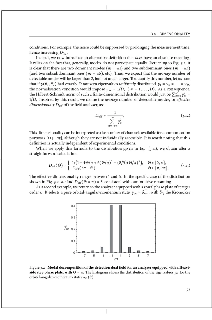
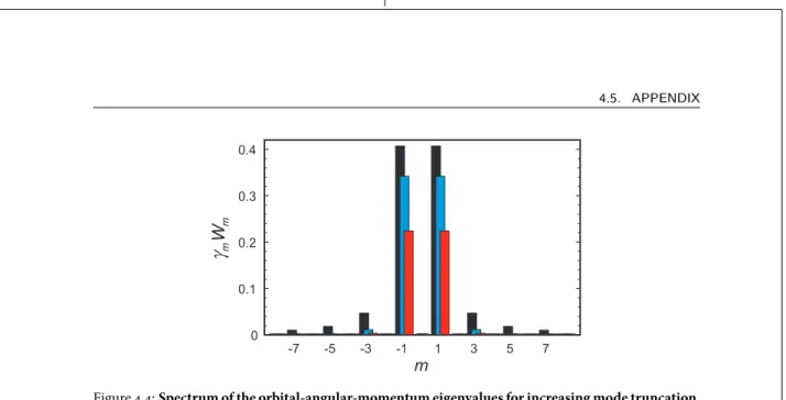
In Fig. 3.2 we show the spectrum of eigenvalues for Θ=π. This distribution contains ample
in-formation about the expected performance of the field analyser. For example, if the input field has no angular dependence, it will not couple at all with this analyser, sinceγ0=0. Secondly, as the Heaviside plate has an anti-symmetric profile on the domain 0 < θ <2π, all even-m
terms vanish.
3.4 Dimensionality
In an actual experimental setting, every field modeum(θ)is subject to a certain amount of
noise. A modeum(θ)can thus only be detected if the analyser’s coupling efficiency to that
3.4. DIMENSIONALITY
conditions. For example, the noise could be suppressed by prolonging the measurement time, hence increasingDfid.
Instead, we now introduce an alternative definition thatdoeshave an absolute meaning. It relies on the fact that, generally, modes do not participate equally. Returning to Fig. 3.2, it is clear that there are two dominant modes(m= ±1)and two subdominant ones(m= ±3)
(and two subsubdominant ones(m= ±5), etc). Thus, we expect that theaveragenumber of
detectable modes will be larger than 2, but not much larger. To quantify this number, let us note that ifγ(θ1,θ2)had exactlyDnonzero eigenvaluesuniformlydistributed,γ1=γ2=. . .=γD, the normalisation condition would imposeγm = 1/D, (m = 1, . . . ,D). As a consequence,
the Hilbert-Schmidt norm of such a finite-dimensional distribution would just be∑
D m=1γ2m= 1/D. Inspired by this result, we define theaveragenumber of detectable modes, oreffective
dimensionality Deffof the field analyser, as:
Deff= 1
∞
∑
m=−∞
γ2m
. (3.12)
This dimensionality can be interpreted as the number of channels available for communication purposes [124, 125], although they are not individually accessible. It is worth noting that this definition is actually independent of experimental conditions.
When we apply this formula to the distribution given in Eq. (3.11), we obtain after a straightforward calculation:
Deff(Θ) = { 1/(1−4Θ/π+6(Θ/π) 2
− (8/3)(Θ/π)3), Θ∈ [0,π],
Deff(2π−Θ), Θ∈ [π, 2π]. (3.13)
The effective dimensionality ranges between 1 and 6. In the specific case of the distribution shown in Fig. 3.2, we findDeff(Θ=π) =3, consistent with our intuitive reasoning.
As a second example, we return to the analyser equipped with a spiral phase plate of integer ordern. It selects a pure orbital-angular-momentum state:γm =δnm, withδi jthe Kronecker
- 7 - 5 - 3 - 1 1 3 5 7
m
0 0.1 0.2 0.3 0.4
m
g
Figure 3.2: Modal decomposition of the detection dual field for an analyser equipped with a Heavi-side step phase plate, withΘ=π.The histogram shows the distribution of the eigenvaluesγmfor the
delta. The resultant effective dimensionality equalsDeff = 1, exposing the inability of this apparatus to probe a multi-dimensional space.
Equation (3.12) is the second main result of this article. It furnishes a simple recipe to calculate the number of modes that an angular phase plate analyser can effectively detect.
3.5 Measuring the effective dimensionality
The effective dimensionality Deff, defined in Eq. (3.12), can actually be measured with the simple experimental setup shown in Fig. 3.3. The setup consists of a mirror-inverted field analyser, oriented atα′, that is imaged by means of a telescope onto a normal field analyser oriented atα. With mirror-inverted field analyser, we mean that the analyser is equipped with an angular phase plate that is a mirrored copy of the normal angular phase plate. More details on the setup can be found in Ref. [119]. With this scheme, we can basically measure the overlap
dual field generator
telescope
dual field analyzer monochromatic
light
a’
a
Figure 3.3: Setup for the determination of the effective dimensionalityDeff. Monochromatic light emerges from a mirror-inverted field analyser oriented at an angleα′, and is coupled into a normal field analyser set atα. The intensity is recorded asαis rotated over 2π. Here, the phase plates have a Heaviside step profile, with Θ=π.
between two analyser modes belonging to different phase plate orientationsαandα′. From the definition of the detection dual field given previously, it follows that the mirror-inverted analyser generates a dual fieldA(θ,α′), when fed from the output port of its fiber. This field is imaged onto the second analyser that selects the dual fieldA(θ,α)and relays an output signal whose power equals
P(α,α′) = ∣∫ 2π
0
A∗(θ,α)A(θ,α′)dθ∣ 2
≡ ∣G(α,α′)∣
2
. (3.14)
The rotational symmetry (see Eq. (3.5)) yields a direct correspondence betweenG(α−α′)and the analyser’s coherence function:G(α,α′) =2πγ(−α,−α′). In fact, it follows that
G(α,α′) =G(α−α′). (3.15)
The coupling strength between the mode generator and mode analyser is, not surprisingly, dependent on therelativeorientation angleα−α′only. The coherence functionG(α,α′)is a measure of theangular sensitivityof a mode analyser, meaning that it characterises how fast the detection mode changes when the phase plate is rotated.
3.6. DISCUSSION
Figure 3.4: Experimental determination of the effective dimensionalityDeff.Experiment performed with a Heaviside step phase plate analyser with Θ=π, by means of the setup depicted in Fig. 3.3. The dots
are experimental data (taken from Ref. [119]) and the solid curve the theoretically predicted∣G(α−α′)∣2.
The value ofDeff is the inverse of the average normalised intensity (equal to 2πdivided by the area underneath the normalised curve).
curve gives the theoretical mode overlap∣G(α−α′)∣2. The coherenceG(α−α′)changes
lin-early with the difference angleα−α′, giving rise to a parabolic intensity curve.
Exploiting the correspondence with γ(α,α′) and its expansion in orbital-angular-momentum eigenmodes, we integrateG(α−α′)over the difference angleα−α′and arrive
at:
Deff= 2π
∫
2π
0 ∣G(α−α′)∣2d(α−α′)
. (3.16)
That is to say, the effective dimensionalityDeffof the detector is just equal to 2πtimes the inverse of the area below the curve of normalised maximum intensity. This shows the exper-imental relevance of the newly defined effective dimensionality. Applying this strategy to the case shown in Fig. 3.4, we find indeedDeff=3.0, in agreement with theory. Equation (3.16) is
the third major result of this article.
3.6 Discussion
We have demonstrated that the angular phase plate analysers under consideration show mul-tiple aspects regarding dimensionality: they are(i)single-mode projectors,(i i)able to access
high-dimensional spaces and,(i i i)characterised by an effective dimensionalityDeff. Here,
we aim to give an intuitive representation of these features.
The key idea in this section is to represent a detection dual fieldA(θ,α)by a complex vector
in the linear, infinite-dimensional spaceUthat is spanned by the orbital-angular-momentum modesum(θ). The detection state vector has components along the ‘axes’um(θ)that carry both amplitude and phase.
is set by the physical shape of the phase plate. Thus, as allγmare fixed, the modal content of the dual field is fixed. This reflects the single-mode detection of the analyser.
However, the performance of these analysers is not determined by a single value ofA(θ,α) calculated for a given value of the continuous parameterα, but rather by thewhole setof fields
{A(θ,α)}α obtained by varyingαbetween 0 and 2π. When the phase plate is rotated, the state vector A(θ,α)redirects, as the phase factors of each field componentum(θ)start to
change. As a result, the set of fields{A(θ,α)}αspans a subspaceUα ⊆Uthat occupies some
‘volume’ withinU. Our effective dimensionalityDeffquantifies this volume, by weighing the eigenmodesum(θ)in the expansion ofA(θ,α)by the square of their coefficientsγm.
In Fig. 3.5 we sketch the behaviour ofA(θ,α)in a cartoon-like manner. For pictorial
convenience, we fix this figure to dim(U) = 3 and we drawA(θ,α)as a real-valued
three-dimensional vector. As the parameterαvaries, such a vector draws a continuous curve within U, and after a 2πrotation ofαit returns at its initial point. The closed curve makes excursions in all three dimensions and so it spans an overall object. When this curve embodies a ball-like volume, as in Fig. 3.5(a), it implies that allγmare approximately equal and the effective dimensionality of this volume is about 3. However, the excursions may not be equally strong along all axes. When the spanned structure spans a plate-like volume, squeezed along a certain direction, as shown in Fig. 3.5(b), its effective dimensionality is about 2. Finally, when the curve covered byA(θ,α)spans a cigar-like space squeezed along two directions, as depicted in Fig. 3.5(c), thenDeff≃1.
3.7 Conclusions
The key results of this article are threefold. First, we have shown that an angular phase-plate analyser can be represented by an angular coherence function (Eq. (3.6)) and we have given its expansion in orbital-angular-momentum eigenmodes. Secondly, we have introduced a novel quantity that gives the effective number of modes that an analyser can access (Eq. (3.12)). Un-like the fidelity dimension, which counts the total number of observable modes in the presence of noise, the effective dimensionality does not depend on experimental conditions. It can be seen as the number of communication channels that an analyser sustains. Lastly, it was shown that the effective dimensionality can easily be obtained experimentally. This important feature is expressed by Eq. (3.16).
3.7. CONCLUSIONS
a)
b)
c)
CHAPTER 4
Shannon dimensionality of quantum channels and its
application to photon entanglement
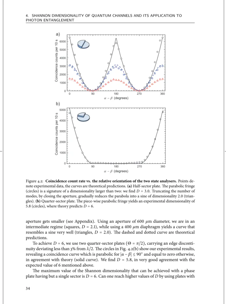
We introduce the concept of Shannon dimensionalityDas a new way to quantify bipartite entanglement as measured in an experiment. This is applied to orbital-angular-momentum entanglement of two photons, using two state analysers composed of a rotatable angular-sector phase plate that is lens-coupled to a single-mode fiber. We can deduce the value ofDdirectly from the observed two-photon coincidence fringe. In our experiment,Dvaries between 2 and 6, depending on the experimental conditions. We predict how the Shannon dimensionality evolves when the number of angular sectors imprinted in the phase plate is increased and anticipate thatD≃50 is experimentally within reach.
J.B. Pors, S.S.R. Oemrawsingh, A. Aiello, M.P. van Exter, E.R. Eliel, G. W. ’t Hooft, and J.P. Woerdman, Physical Review Letters101, 120502 (2008)