Stochastic Optimization Using Continuous Action-Set Learning Automata

Stochastic Optimization Using Continuous

Action-Set Learning Automata

H. Beigy

and M.R. Meybodi 1

In this paper, an adaptive random search method, based on continuous action-set learning automata, is studied for solving stochastic optimization problems in which only the noise-corrupted value of a function at any chosen point in the parameter space is available. First, a new continuous action-set learning automaton is introduced and its convergence properties are studied. Then, applications of this new continuous action-set learning automata to the minimization of a penalized Shubert function and pattern classication are presented.

INTRODUCTION

Optimization with noisy corrupted measurements is a common problem in many areas of engineering. Con-sider a system with measurements ofg(x), whereis the parameter andxis the observation. The parameter optimization problem is dened so as to determine the optimal parameter,, such that the performance function, M() = Eg(x)], is optimized. Many ecient methods, like the steepest descent method and Newton's method, are available when gradient,rM, is explicitly available. Usually, due to the lack of sucient information concerning the structure of functionM or because of mathematical intractability, functionM to be optimized is not explicitly known and only the noise-corrupted value of functionM() at any chosen point,

, can be observed. Two important classes of algorithm are available for solving the optimization problem when only the noise-corrupted observations are available: Stochastic approximation based algorithms 1] and learning automata based algorithms 2,3].

Stochastic approximation algorithms are iterative algorithms in which the gradient of function, M, is approximated by a nite dierence method and using the function evaluations obtained at points, which are chosen close to each other 1]. Learning automata are adaptive decision making devices that operate in unknown random environments and progressively improve their performance via a learning process.

*. Corresponding Author, Department of Computer Engi-neering, Sharif University of Technology, Tehran, I.R. Iran.

1. Department of Computer Engineering, Amir Kabir Uni-versity of Technology, Tehran, I.R. Iran.

Learning automata are very useful for optimization of multi-modal functions when the function is unknown and only noise-corrupted evaluations are available. In these algorithms, a probability density function, which is dened over the parameter space, is used for selecting the next point. The reinforcement signal and the learning algorithm are used by learning automata for updating the probability density function at each stage. It is required that this probability density function con-verge to some probability density function where the optimal parameter, , is chosen with probability as being as close as possible to unity. The distinguishing feature of the learning is that probability distribution ofg(x) is unknown.

Methods based on stochastic approximation al-gorithms and learning automata represent two dis-tinct approaches to learning problems. Though both approaches involve iterative procedures, updating at every stage is done in the parameter space in the rst method, which may result in a local optimum, and in the probability space in the second method. Learning automata methods have two distinct advantages over the stochastic approximation algorithms. The rst advantage is that the action space need not be a metric space because, as in stochastic approximation algo-rithms, the new value of the parameter is to be chosen close to the previous value. The second advantage is that the methods based on learning automata lead to global optimization, because, at every stage any element of the action-set can be chosen.

In this paper, an adaptive random search method for nding the global minimum of an unknown function is studied. In the rst part of the paper, a new Continuous Action-set Learning Automaton (CALA) is introduced and its convergence behavior is

stud-ied. A strong convergence theorem for this learning automaton is stated and proven. In the second part of the paper, algorithms are proposed, which use the proposed CALA for stochastic optimization of a penalized Shubert function and pattern classication. The proposed algorithm is a constant step size learning algorithm and needs only one function evaluation at each stage. The proposed algorithm is independent of the dimension of the parameter space of the function to be optimized.

The rest of this paper is organized as follows: In the next section a brief review of learning automata is presented. Then, a new continuous action-set learning automaton is given and its behavior is studied. After that, algorithms for stochastic optimization and the experiments are given. Finally, the paper is concluded.

LEARNING AUTOMATA

Learning Automata (LA) are adaptive decision making units that can learn to choose the optimal action from a set of actions by interaction with an unknown random environment. At each instant, n, the LA chooses an action,n, from its action probability distribution and applies it to the random environment. The random environment provides a stochastic response, which is called a reinforcement signal, to the LA. Then, the LA uses the reinforcement signal and learning algorithm to update the action probability distribution.

Learning automata can be classied into two main groups: Finite Action-set Learning Automata (FALA) and Continuous Action-set Learning Au-tomata (CALA) 4]. The action-set of FALA is nite and the action probability distribution is represented by a probability vector that is updated by a learning algorithm. Several algorithms for learning optimal parameters have been developed for many discrete and continuous parameters 2,3,5-7]. When the FALA is used for solving optimization problems, one needs to discretize the parameter space, so that actions of LA can be possible values of the corresponding parameter. The accuracy of the solution is increased by choosing the ner discretization and, hence, increasing the number of actions of LA. However, increasing the number of actions leads to slow convergence of the learning algorithm. A more satisfying solution would be to employ an LA model where the action-set can be continuous, such as a subaction-set of real line. Such a model of LA is called a continuous action-set learning automaton. Like FALA, CALA also use a probability distribution function to choose an action and the learning algorithm updates this function based on the reinforcement signal.

Continuous action-set learning automata that are presented in 8] at instantnuse a normal distribution with mean,n, and standard deviation,n, for action

probability distribution. At each instant, the CALA updates its action probability distribution by updating

nandn. This CALA interacts with the environment through a choice of two actions at each instant. At each instant, n, the CALA choosesn2<at random from its current distribution, N(nn). Then, it gets reinforcement from the environment for the two actions: n andn. Let these reinforcements be() and(). Then, the action probability distribution is updated as:

n+1=n+af1nnn()()]

n+1=n+af2nnn()()];Can;L] (1) wheref1(:)f2(:) and(:) are dened as below:

f1(()()) =

();()

()

;

()

f2(()())=

();()

()

"

;

() 2

;1 #

() = (;L)If > Lg+L (2) and L > 0C > 0 and a 2 (01) are parameters of the algorithm. The learning algorithm for CALA is described below. Since the updating given for n does not automatically guarantee that n+1 n, a projected version of n is always used, denoted by

n]. For this algorithm, it is shown that with an arbitrary large probability, n will converge close to the optimal action and n will converge close to L, provided one chooses and L suciently small and

C suciently large 8].

Continuous Action Reinforcement Learning Au-tomaton (CARLA) is introduced in 9,10]. Let the action-sets of an automaton be a bounded con-tinuous random variable dened over the interval minmax] 2 <. CARLA uses a continuous proba-bility density function, f(n), to choose its actions. It is assumed that no information about the actions is available at the start of learning and, therefore, the action probabilities have uniform distribution. CARLA updatesf(n) according to the following rule.

f(n+ 1) = (

af(n)+(1;n)H(n)] if n2maxmin]

0 otherwise ₍₃₎

where a is a normalization factor, n 2 01] is the reinforcement signal and H(r) is a symmetric Gaussian neighborhood function centered on r = n given by H(r) = e;

1 2(

;r )

2

parameters that aect the height and the width of this neighborhood function.

Gullapalli proposed a generalized learning au-tomaton with a continuous action-set, which uses the context input for selecting its actions and the reinforce-ment signal for updating its parameters 11]. Vasilakos et al. introduced a generalized learning automaton with a continuous action-set and has shown that this learning automaton nds the optimal action for each context vector 12]. In 13], a team of FALA and CALA is also used for stochastic optimization.

Learning automata have been used successfully in many applications, such as computer networks 14-16], solving NP-complete problems 17-19], capacity assignment 20,21], neural network engineering 22-25], and cellular networks 26-29] to mention a few.

A NEW CONTINUOUS ACTION-SET

LEARNING AUTOMATON

In this section, a new Continuous Action-set Learning Automaton (CALA) is introduced, which will be used later in the paper for stochastic optimization. For the proposed CALA, the Gaussian distribution,N(nn), is used for selection of actions, which is completely specied by the rst and second order moments, n andn. The learning algorithm updates the mean and variance of the Gaussian distribution at any instant, using the reinforcement signal, , obtained from the random environment. The reinforcement signal, 2 01], is a noise-corrupted reinforcement signal, which indicates a noise-corrupted observation of function

M(:) at the selected action. The reinforcement signal,

, is a random variable whose distribution function coincides almost with the distribution, H(j), that belongs to a family of distributions which depends on the parameter. Let:

M() = E()j] = Z

1 ;1

()dH(j)

be a penalty function with boundMcorresponding to this family of distributions. It is assumed that M(:) is measurable and continuously dierentiable almost everywhere. The CALA has to minimize M(:) by observing (). Using the learning algorithm, one ideally requires that n !

and

n ! 0, as time tends to innity.

The interaction between the CALA and the random environment takes place as iterations of the following operations. Iterationnbegins by selection of an action,n, by the CALA. This action is generated as a random variable from the Gaussian distribution with parametersnandn. The selected action is applied to the random environment and the learning automaton receives an evaluative signal, (n), which has the

mean value,M(n), from the environment. Then, the learning automaton updates the parametersnandn. Initially, M(:) is not known and it is desirable that with the interaction of the learning automaton and the random environment, and converge to their optimal values, which results in the minimum value of

M(:). The learning automaton uses the following rule to update parameters n and n, thus, generating a sequence of random variables,n andn:

n+1=n;a(n)n(n;n)

n+1=f(n) (4) whereais learning rate andf(:) is a function that pro-duces a sequence offng(described later). Equation 4 can be written as:

n+1=n;a

2

nyn(n) (5)

where:

yn(n) =(n)

n;n

n

: (6)

An intuitive explanation for the above updating equa-tions is as follows. One can view the fraction in Equation 6 as the normalized noise added to the mean. Sinceaandare all positive, the updating equation changes the mean value in the opposite direction of the noise. If the noise is positive, then the learning automaton should update its parameter, so that mean value increases and vice versa. Since Ej] is close to unity when is far from its optimal value and is close to zero whenis near to the optimal value, the learning automaton updates with large steps when

is far from its optimal value and with small steps when is close to its optimal value. This causes a ner quantization of near its optimal value and a grain quantization for points far away from its optimal value. Thus, one can consider the learning algorithm as a random direction search algorithm with adaptive step sizes.

In what follows, the convergence of the pro-posed learning automaton in stationary environments is stated and proven. The convergence is proven, based on the following assumptions.

Assumption 1

The sequence of real numbers,fng, is such thatn 0P

1

n=1n3=1and P

1

n=1n4<1.

Note that these conditions imply that n ! 0 as n ! 1. Therefore, in limit, n of Gaussian distribution tends to zero and the action of the learning automaton becomes equal to the mean. The condition P

1

n=13n =1 ensures that the sum of increments to the initial mean, 0, can be arbitrarily large, so that

the optimal value,. At the same time, the condition P

1

n=1n4<1ensures that the variance inn is nite and the mean cannot diverge to innity. Here, 2

is like the step size, thus, the above is the standard assumption in stochastic approximation algorithms on the step size.

Assumption 2

M() has a unique minimum at. LetR() =@M()

@

and S() = @M2()

@2 be the rst and the second derivative of M(), respectively. M() has a nite number of minima inside a compact set. M()R() andS() have bounds M,RandS, respectively.

Note that this assumption ensures that there is an optimal action, , for the learning automaton for which E()] is minimum. Since, in limit,

n !0, then, this assumption ensures that there is an optimal mean,, for whichM is minimized.

Assumption 3

M() is linear near , that is sup

"j;

j 1 "(

;

)R()>0for all" >0.

Assumptions 2 and 3 mean that the function being optimized has a unique minimum and behaves like a quadratic in the search area and near the optimum point.

Assumption 4

The noise in the reinforcement signal, (:), has a bounded variance, that is:

En

();M()]

2o K1

1 + (;

)2 (7) for some real number,K1>0.

Given the above assumptions, in what follows, the behavior of the proposed CALA is studied. The following theorem states the convergence of the random process dened by Equation 4. The method used to prove this theorem is similar to the methods used in stochastic approximation 1].

Theorem 1

Suppose that Assumptions 1 to 4 hold,0is nite and

there is an optimal value offor. Then, if

nandn are evolved according to the given learning algorithm, then, limn!1n =

with probability 1.

Before the above theorem is proven, rst, the following two lemmas are proven.

Lemma 1

Eyn(n)jn] =nR(n):

Proof

Let n denote (n), where n is a random variable chosen from Gaussian distribution with mean n and

variance_n2_.

Eyn(n)jn] = E

M(n)

n;n

n n : (8) ReplacingM(n) with its second order Taylor se-ries expansion aroundn and simplifying, one obtains:

Eyn(n)jn] =M(n)E

n;n

n n +R(n)E

(n;n)2

n n + 12E

S()

(n;n)3

n n

where lies between n and n. The rst and last terms on the right hand side of the above equation are zero, because the odd moments of a Gaussian random variable, n, are zero. Since M(:) has a bounded second derivative, the above equation can be written as Eyn(n)jn] =nR(n):

Lemma 2

E

y_n2_(n)jn K2

1 + (n; )2 :

Proof

E

y_n2_(n)

jn = Z 1 ;1 E ( n

n;n

n 2 n )

dN(njnn) = Z 1 ;1 E _n2 n

n;n

n

2

dN(njnn): (9) By substituting Inequality 7 in the above equation, one obtains:

E

y_n2_(n)

jn K1

Z 1 ;1

1 + (n;

)2+M2(

n)

n;n

n

2

dN(njnn) =K1

Z 1 ;1

1+M2_(n)

n;n

n

2

dN(njnn) +K1

Z 1 ;1

(n;n)2+ 2(n;n)(n; ) + (n;

)2

n;n

n

2

Since the odd moments of a Gaussian random variable are zero, the above equation can be written as:

Eh

y_n2_(n)

jn i

K1+ 3K1

2

n+K1(n; )2 +K1

Z 1 ;1

M2_(n)

n;n

n

2

dN(njnn): (10) Replacing M(n) with its second order Taylor series expansion aroundn and using the fact that M and its rst and second derivatives are bounded, the last term of the above equation is equal to:

Z 1 ;1

M2_(n)

n;n

n

2

dN(njnn)

Z

1 ;1

M+R(n;n) +S

(n;n)2 2

2

n;n

n

2

dN(njnn)

(11) where lies between n and n and R and S are bounds of the rst and the second derivative ofM(:), respectively. Using the fact that the odd moments of a Gaussian random variable are zero, the above inequality can be simplied as:

Z 1 ;1

M2_(n)

n;n

n

2

dN(njnn)

M

2_{+ 3}

R

2_n2_{+ 3}

MS

2

n+ 154S

2_n4_:

Substituting the above equation in Equation 10, one obtains:

E

y2_n(n)

jn K1+ 3K1

2

n+K1(n; )2 +K1M

2_{+ 3K1}

R

2_n2_{+ 3K1}

MS

2

n + 154K1S

2_n4_:

Since nMR andS are bounded random variables, there is a constant K2 > 0, such that the above

inequality can be written as: E

y2_n(n)

jn K2 ;

1 + (n; )2

: (12)

Proof of Theorem 1

Leten =n;

. Then using Equation 5, e

n can be dened recursively as:

en+1=en;a

2

nyn(n): (13)

Squaring, taking the conditional expectation given in

0n of both sides of the recursive formula for

en+1 and, then, using Lemmas 1 and 2, one obtains:

Eh

e2_n+1

j0n i = E

;

en;a

2

nyn(n)2 0 n e 2

n+a2K2n4(1 +e2n);2a

2_K2n3_enR(n)

e

2

n+a2K24n(1 +e2n) =e2_n;

1 +a2_K24_n

+a2_K2n4_{: (14)}

Let:

Zn=e2n

1 Y

j=n

;

1+a2_K24_j

+a2_K21 X

j=n

4

j

1 Y

i=j+1

;

1+a2_K2i4

:

(15) Then, using Equation 15, it is easy to show that

e2_n Zn and EfZn+1j0ng Zn: Tak-ing the conditional expectations given, Z1Zn, on both sides of the above inequality, one obtains EfZn+1jZ0Zng Zn which shows that Zn is a non-negative super-martingale. Thus, one has EfZn+1g EfZng EfZ1g 1: Therefore, using the martingale convergence theorems 30], Zn converges with probability 1. Since e2_n Zn, hence one concludes thate2_{nconverges towith probability 1,}

where <1is a random variable. Taking expectation on both sides of Equation 14, one obtains:

E

e2_n+1

;E

e2_n

a

2_K24_n; 1 + E

e2_n

;2a2K2n3enR(n):

Adding the rstnof these inequalities, one gets: E

e2_n+1

;E

e21 a

2_K2Xn

j=1 4

n; 1 + E

e2_j

;2a2K2

n

X

j=1 3

jejR(j): Adding E

e₂₁ to both sides of the above inequality, one obtains:

E

e2_n+1 E

e21 +a2_K2Xn

j=1 4

n; 1 + E

e2_j

;2a

2_K2Xn

j=1 3

Since E

e2_{n+1 is positive, the above inequality}

be-comes: E

e21+a2_K2Xn

j=1 4

n; 1+E

e2_j

;2a

2_K2Xn

j=1 3

jejR(j)0: From the above inequality, using the boundness of E

e2_{j (forj >0) and Assumption 1, it follows that:}

2a2_K2Xn

j=1 3

jejR(j)E

e21 +Xn

j=1a

2_K2n4; 1+E

e2_j

<1: Since P

1

j=13j diverges and, by Assumption 3, the quantity of ejR(j) is positive, one can conclude that for some sequence, fnjg, one has en

jR(nj) ! 0, with probability 1. The fact that e2_{n converges with}

probability 1 to some random variable, , together with Assumptions 1 through 4 and the above equation, it implies that = 0 with probability 1. Hence, n converges to with probability 1.

NUMERICAL EXAMPLES

In this section, the application of the proposed con-tinuous action-set learning automaton is studied. Two problems are studied: The rst problem is to nd a minimum of the penalized Shubert function, when the function evaluations are corrupted by noise, and the second problem is to nd an optimal discriminant func-tion for pattern classicafunc-tions. In both problems, only the function evaluations are assumed to be available.

Optimization of a Function

In this section, an algorithm is given, based on the proposed continuous action-set learning automaton, for optimization of an unknown function. The pro-posed algorithm can be easily extended to multivariate functions by using a cooperative game of CALA with identical payo. Consider a function F : < ! < to be minimized. At any instant, n, the automaton chooses an action,n, using the Gaussian distribution,

N(nn), where n and n are the mean and the standard deviation, respectively. As before, let () denote the noisy function evaluation at point 2 <, such that () = f();

2

1 , where 1 and 2 are two appropriate scaling constants, such that (a) 2 01] andf(:) is a noisy evaluation ofF(a). This is because of the assumption thatis a bounded and nonnegative random variable. The signal () is used to update

of the Gaussian distribution (Equation 4).

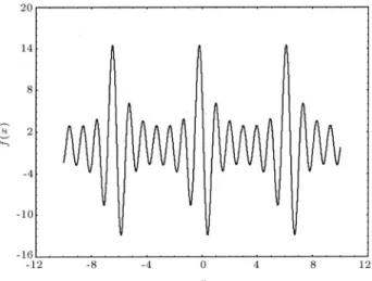
In order to study the behavior of the proposed algorithm, one must consider the optimization of the penalized Shubert function, which is borrowed from 8],

when the function evaluations are noisy. The penalized Shubert function (Figure 1) is frequently used as one of the benchmark problems for global optimization problems. The penalized Shubert function is given below:

F(x) =X5

i=1icos((i+ 1)x+ 1) +u(x101002) (16)

whereuis the penalizing function, given by:

u(xbkm) = 8 > < > :

k(x;b)m x > b

0 jxjb

k(;x;b)m x <;b

: (17) This function has 19 minima within interval ;1010], where three of them are global minima. The global minimum value of the penalized Shubert function is approximately equal to -12.87 and is attained at points close to -5.9, 0.4 and 6.8.

The proposed continuous action-set learning au-tomaton and the auau-tomaton proposed in 8], with dierent initial values of the mean and variance param-eters, are used for nding the minimum of the penalized Shubert function. The algorithm given in 8] is used with the following values of parameters: The penalizing constant, C, is equal to 5, the lower bound for the variance, L = 0:01 and the step size a = 2 10;4. The proposed algorithm is used with a = 0:01 and the variance is updated according to the following equation:

n = 1

b10nc1=3

where b:c denotes the oor function. It can be easily veried that sequence fng satises the conditions of Assumption 1. From the denition of the reinforcement

Table 1. The simulation results with noiseU;0:50:5] added to the penalized Shubert function evaluations.

Case Initial Values

Proposed Algorithm

Old Algorithm

0

0

8000

8000

F

(

8000

)

8000

8000

F

(

8000

)

1 4 6 6.716046 0.1 -12.861304 2.534 0.01 -3.578

2 4 10 0.436827 0.1 -12.848987 0.4308 0.01 -12.87

3 8 5 7.805426 0.1 -3.5772 5.364 0.01 -8.5

4 8 3 6.704283 0.1 -12.868272 6.72 0.01 -12.87

5 12 6 5.460669 0.1 -8.476369 1.454 0.01 -3.58

6 -10 5 -8.107043 0.1 -3.749682 -7.1 0.01 -8.5

7 -10 6 -7.09686 0.1 -8.507154 -5.8 0.01 -12.87

signal , it is clear that the highest expected rein-forcement is 1.0 and the lowest expected reinrein-forcement is 0.0 for either evaluation. It is easy to see that

M() = Ej] and satisfy Assumptions 2 through 4. The function evaluations are corrupted by a zero mean noise randomly generated from uniform and normal distributions. The results of simulation for two algorithms, when noise is in the range -0.5,0.5] with uniform distribution, are shown in Table 1, i.e.

f(x) =F(x) +U;0:50:5], whereUab] is a random number in interval ab] with uniform distribution. The results of simulation for two algorithms when noise has normal distribution are shown in Tables 2 through 11, i.e. f(x) =F(x)+N(0), whereN(0) is a random number with uniform distribution with zero mean and the variance of . The simulation results show that the mean values of Gaussian distribution used in CALA always converge to a minimum of the penalized Shubert function within the interval -10,10], which has a higher rate of convergence than the algorithm given in 8].

By comparing the results of simulations for both algorithms, one concludes that two algorithms have approximately the same accuracy, but the proposed

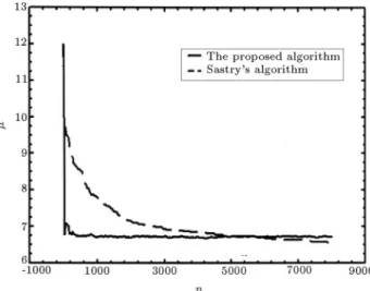
Figure2. The convergence of the mean value of the Gaussian distribution for uniform noise.

Figure3. The convergence of the mean value of the Gaussian distribution for noise with normal distribution.

algorithm has a higher speed of convergence. Figures 2 and 3 show the changes in versusnfor typical runs for the proposed algorithm and the algorithm given in 8], when noise with uniform or normal distribution is added to the function evaluations. These gures show that the proposed algorithm converges to a minimum quickly and has oscillations around the minimum point. However, such oscillations could be decreased by using a small step size, which results in decreasing the rate of convergence.

Pattern Classication

In this section, an algorithm, based on the proposed continuous action-set learning automaton for solving pattern classication problems is given. A pattern classication problem can be formulated as follows: There is a set of patterns that must be classied into a nite number of classes. The information about a pattern is summarized by a d-dimensional vector,

X = x1x2xd]

T_{, called a feature vector. Let}

m possible pattern classes be !1!2!m. Let

Table 2. The simulation results with white noiseN(00:1) added to the penalized Shubert function evaluations.

Case Initial Values

Proposed Algorithm

Sastry's Algorithm

0

0

8000

8000

F

(

8000

)

8000

8000

F

(

8000

)

1 4 6 6.725683 0.107958 -12.82271 6.735791 2.204917 -12.75081 2 4 10 6.727295 0.107958 -12.813384 9.213571 0.624627 2.763267

3 8 5 -5.84428 0.107958 -12.840563 10 0.038636 -0.002154

4 8 3 0.45588 0.107958 -12.720715 9.561054 0.188162 -0.731982

5 12 6 -5.86847 0.107958 -12.853415 10 0.014074 -0.002154

6 -10 5 6.714694 0.107958 -12.864359 -9.610859 0.251364 2.879572 7 -10 6 -5.86368 0.107958 -12.865793 -9.612072 0.085958 2.875568 Table 3. The simulation results with white noiseN(00:2) added to the penalized Shubert function evaluations.

Case Initial Values

Proposed Algorithm

Sastry's Algorithm

0

0

8000

8000

F

(

8000

)

8000

8000

F

(

8000

)

1 4 6 4.449063 0.107958 -3.739168 6.774669 2.23965 -12.185001

2 4 10 6.729869 0.107958 -12.79681 10 0.059367 -0.002154

3 8 5 0.427261 0.107958 -12.87015 10 0.023405 -0.002154

4 8 3 6.696855 0.107958 -12.84972 10 0.023574 -0.002154

5 12 6 -8.10426 0.107958 -3.749953 9.999982 0.021554 -0.002484 6 -10 5 6.704349 0.107958 -12.86835 -9.630264 0.261474 2.795851 7 -10 6 -5.84628 0.107958 -12.84872 -9.624987 0.234517 2.822746 Table 4. The simulation results with white noiseN(00:3) added to the penalized Shubert function evaluations.

Case Initial Values

Proposed Algorithm

Sastry's Algorithm

0

0

8000

8000

F

(

8000

)

8000

8000

F

(

8000

)

1 4 6 5.46562 0.1079 -8.4960 6.6935 2.103081 -12.8358

2 4 10 6.70878 0.1079 -12.8701 10 0.037497 -0.00215

3 8 5 -8.1126 0.1079 -3.7457 10 0.04331 -0.00215

4 8 3 -5.8514 0.1079 -12.8638 10 0.017517 -0.00215

5 12 6 -7.1112 0.1079 -8.4467 10 0.021286 -0.00215

6 -10 5 6.72450 0.1079 -12.829 -9.6049 0.200885 2.898331

7 -10 6 -5.8533 0.1079 -12.8673 -9.6325 0.2594 2.783257

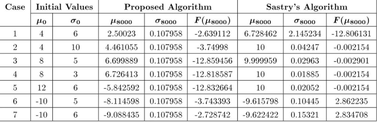
Table5. The simulation results with white noiseN(00:4) added to the penalized Shubert function evaluations

Case Initial Values

Proposed Algorithm

Sastry's Algorithm

0

0

8000

8000

F

(

8000

)

8000

8000

F

(

8000

)

1 4 6 2.50023 0.107958 -2.639112 6.728462 2.145234 -12.806131

2 4 10 4.461055 0.107958 -3.74998 10 0.04247 -0.002154

3 8 5 6.699889 0.107958 -12.859456 9.999959 0.02963 -0.002901

4 8 3 6.726413 0.107958 -12.818587 10 0.01885 -0.002154

5 12 6 -5.842592 0.107958 -12.832664 10 0.02052 -0.002154

6 -10 5 -8.114598 0.107958 -3.743393 -9.615798 0.10445 2.862235 7 -10 6 -9.088435 0.107958 -2.728742 -9.622422 0.15321 2.834708

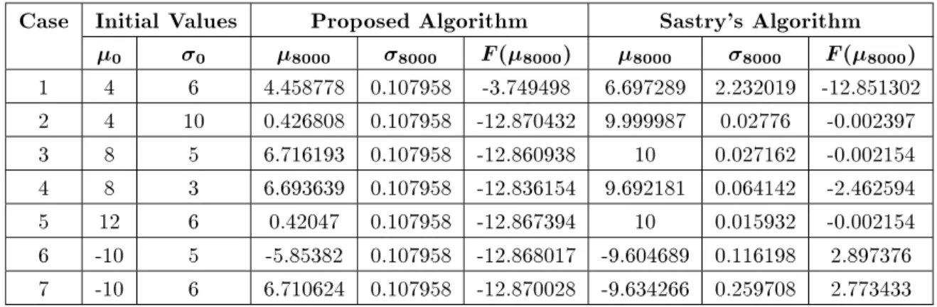
Table6. The simulation results with white noiseN(00:5) added to the penalized Shubert function evaluations.

Case Initial Values

Proposed Algorithm

Sastry's Algorithm

0

0

8000

8000

F

(

8000

)

8000

8000

F

(

8000

)

1 4 6 4.458778 0.107958 -3.749498 6.697289 2.232019 -12.851302 2 4 10 0.426808 0.107958 -12.870432 9.999987 0.02776 -0.002397

3 8 5 6.716193 0.107958 -12.860938 10 0.027162 -0.002154

4 8 3 6.693639 0.107958 -12.836154 9.692181 0.064142 -2.462594

5 12 6 0.42047 0.107958 -12.867394 10 0.015932 -0.002154

6 -10 5 -5.85382 0.107958 -12.868017 -9.604689 0.116198 2.897376 7 -10 6 6.710624 0.107958 -12.870028 -9.634266 0.259708 2.773433

Table 7. The simulation results with white noiseN(00:6).

Case Initial Values

Proposed Algorithm

Sastry's Algorithm

0

0

8000

8000

F

(

8000

)

8000

8000

F

(

8000

)

1 4 6 5.480349 0.089604 -8.517418 4.055911 20.009987 2.400759 2 4 10 0.435484 0.089604 -12.85371 4.054561 20.00997 2.415684 3 8 5 6.726655 0.089604 -12.81718 8.006934 20.009995 -0.62230 4 8 3 6.709202 0.089604 -12.87075 8.003345 20.009943 -0.70354 5 12 6 9.756602 0.089604 -2.727776 9.999975 20.009989 -0.00260 6 -10 5 -9.98241 0.089604 -2.205438 -9.93990 20.009995 -1.70987 7 -10 6 -7.09524 0.089604 -8.510625 -9.94036 20.009991 -1.71605

Table 8. The simulation results with white noiseN(01:3).

Case Initial Values

Proposed Algorithm

Sastry's Algorithm

0

0

8000

8000

F

(

8000

)

8000

8000

F

(

8000

)

1 4 6 6.70339 0.089604 -12.8669 4.05304 20.009989 2.432262

2 4 10 0.43157 0.089604 -12.8642 4.05334 20.009985 2.428998

3 8 5 6.72627 0.089604 -12.8193 8.01151 20.009995 -0.51832

4 8 3 6.72909 0.089604 -12.8020 7.99121 20.009989 -0.97549

5 12 6 9.76507 0.089604 -2.72765 9.99998 20.009995 -0.00251 6 -10 5 -9.9842 0.089604 -2.22347 -9.9406 20.009995 -1.72048 7 -10 6 -9.9838 0.089604 -2.21967 -9.9455 20.009995 -1.78518

Table 9. The simulation results with white noiseN(01:9).

Case Initial Values

Proposed Algorithm

Sastry's Algorithm

0

0

8000

8000

F

(

8000

)

8000

8000

F

(

8000

)

1 4 6 6.731426 0.089604 -12.78577 4.05399 20.009993 2.421903 2 4 10 6.685631 0.089604 -12.78776 4.05446 20.009977 2.416788 3 8 5 6.723327 0.089604 -12.83486 8.00724 20.009989 -0.61527 4 8 3 6.715631 0.089604 -12.86230 7.99826 20.009981 -0.81798 5 12 6 9.760613 0.089604 -2.728751 9.99999 20.009993 -0.00232 6 -10 5 -9.98213 0.089604 -2.202685 -9.9434 20.009998 -1.75658 7 -10 6 -9.98342 0.089604 -2.215217 -9.9444 20.009991 -1.77056

Table10. The simulation results with white noiseN(02:6).

Case Initial Values

Proposed Algorithm

Sastry's Algorithm

0

0

8000

8000

F

(

8000

)

8000

8000

F

(

8000

)

1 4 6 5.47063 0.089604 -8.50962 4.054261 20.00998 2.418973

2 4 10 5.45497 0.089604 -8.44608 4.053005 20.00997 2.432638

3 8 5 6.70863 0.089604 -12.8708 8.005559 20.01000 -0.65347

4 8 3 6.72332 0.089604 -12.8348 8.004089 20.00998 -0.68673

5 12 6 9.77867 0.089604 -2.71016 9.999991 20.00999 -0.00231 6 -10 5 -9.9827 0.089604 -2.20913 -9.94208 20.01001 -1.73909 7 -10 6 -5.8538 0.089604 -12.8679 -9.94117 20.00996 -1.72688

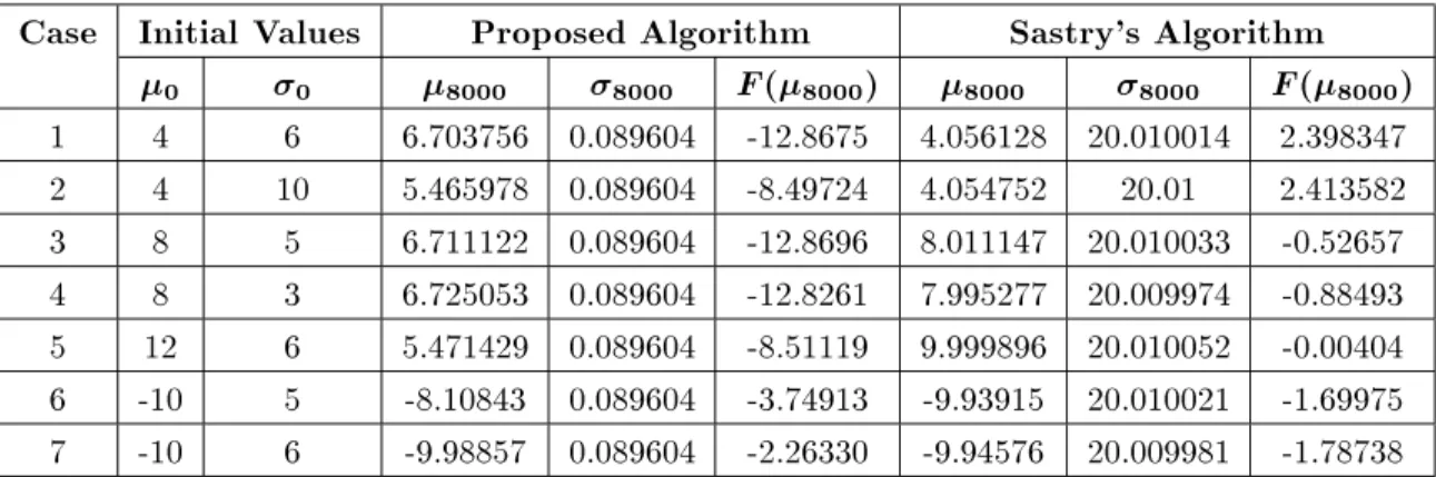
Table11. The simulation results with white noiseN(03:2).

Case Initial Values

Proposed Algorithm

Sastry's Algorithm

0

0

8000

8000

F

(

8000

)

8000

8000

F

(

8000

)

1 4 6 6.703756 0.089604 -12.8675 4.056128 20.010014 2.398347

2 4 10 5.465978 0.089604 -8.49724 4.054752 20.01 2.413582

3 8 5 6.711122 0.089604 -12.8696 8.011147 20.010033 -0.52657 4 8 3 6.725053 0.089604 -12.8261 7.995277 20.009974 -0.88493 5 12 6 5.471429 0.089604 -8.51119 9.999896 20.010052 -0.00404 6 -10 5 -8.10843 0.089604 -3.74913 -9.93915 20.010021 -1.69975 7 -10 6 -9.98857 0.089604 -2.26330 -9.94576 20.009981 -1.78738

i = 1m) be the class conditional densities. The function of a pattern classier is to assign the correct class membership to each given feature vector,X. Such an operation can be interpreted as a partition of thed -dimensional space into m mutually exclusive regions. The partition boundary can be expressed in terms of discriminant functions. The forms of discriminant functions are assumed to be known, except for some parameter vectorsWi _{(fori= 12}m), which are to be identied. Associated with each class, !i, a discriminant function, di(XWi) (fori= 12m), is selected, such that if patternX were from class !i, then, one would have:

di(XWi)> dj(XWj) 8j6=i (18) where Wi _{is the parameter vector for discriminant} function di.

In this example, the learning pattern classication for a 2-class 2-dimension pattern classication problem is considered. For this problem, one discriminant function, denoted by d(XW) is sucient. In order to nd parameters of the discriminant function, W, a cooperative game of continuous action-set learning automata with identical payo is used. In the proposed method, the teacher (environment) chooses a pattern,

X, randomly based on a priori probabilities. The statistical properties of the pattern classes are assumed to be unknown to the algorithm. The team of learning automata chooses their actions, which result in the determination of parameter vectorW. The parameter vector W, together with feature vector X, determine the classication. The decision rule for pattern classi-cation is formulated as:

!= (

!1 ifd(XW)>0

!2 otherwise (19)

where X = x1x2]T is the feature vector. The

only feedback to the team of continuous action-set learning automata is the reinforcement signal, which is computed according to the following rule:

= (

1 if!6= ^w

0 otherwise (20)

where !is the classication of feature vector X. The objective is to minimize the probability of misclassi-cation of patternX (EjX]), where the expectation is with respect to statistical distribution on the pattern classes. Note that this criterion is a function of the parameter vector,W, which is to be identied.

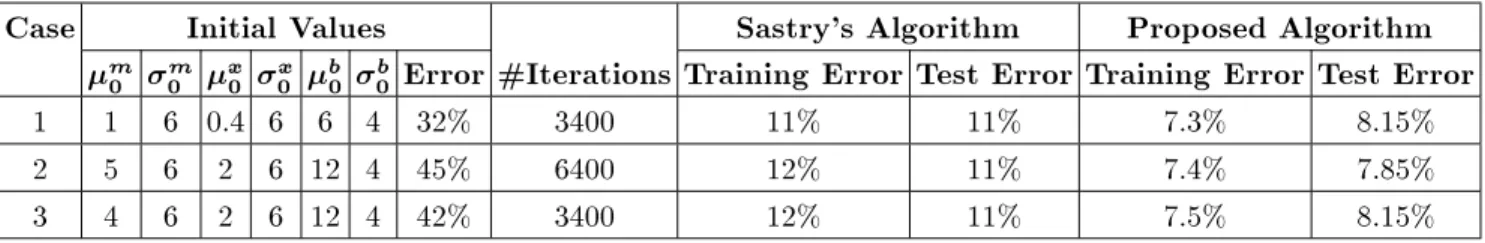
Table12. The simulation results for pattern classication problem.

Case

Initial Values

Sastry's Algorithm

Proposed Algorithm

m 0

m 0

x 0

x 0

b 0

b

0

Error #Iterations Training Error Test Error Training Error Test Error

1 1 6 0.4 6 6 4 32% 3400 11% 11% 7.3% 8.15%

2 5 6 2 6 12 4 45% 6400 12% 11% 7.4% 7.85%

3 4 6 2 6 12 4 42% 3400 12% 11% 7.5% 8.15%

Let the class conditional densities for the two classes be given by the Gaussian distributions

P(Xj!1) = N(m11) and P(Xj!2) = N(m22), where:

m1= 22]T m2= 44]T

1=

1 ;0:25 ;0:25 1

2=

1:5 ;0:25 ;0:25 1:5

:

The following discriminant function is considered for this problem:

g(X) =

"

mx2+x1;(m2+ 1)

x0;

b

(1+m2₎1=2

!#2 1 1 +m2

; "

x1;

x0+_{(1 +m}b₂₎₁₌₂

!#2

; "

x2;m

x0+_{(1 +m}b₂₎₁₌₂

!#2

:

This function is a parabola described by three parameters, mx0 and b. The parameters of the

optimal discriminant function for the above pattern classication problems are m = 1:0x0 = 3:0 and

a = 10:0. For solving this problem, a team of three CALA are used, where each CALA is associated with one unknown parameter. The other parameters for the CALA used in this algorithm are the same as the parameters used in the previous section. For learning, 300 samples of pattern are chosen from each class, which are presented repeatedly to the team of CALA during the training process. Also, a test set consisting of 100 samples is generated from the two classes to nd errors by the chosen discriminant function. The results of simulation for the proposed algorithm and the algorithm given in 8] are shown in Table 12. By carefully inspecting Table 12, it can be concluded that the proposed algorithm has smaller training and generalization errors.

CONCLUSIONS

In this paper, a random search algorithm for solving stochastic optimization problems has been studied. A class of problems has been considered where the only available information is noise-corrupted values of the function. In order to solve such problems, a new continuous action-set learning automaton was proposed and its convergence properties were stud-ied. A strong convergence theorem for the proposed learning automaton was stated and proved. Finally, algorithms for two stochastic optimization problems were given and their behavior was studied through computer simulations. Computer simulations showed that the proposed method has a higher performance compared with existing continuous action-set learning automata based on optimization algorithms.

ACKNOWLEDGMENT

This research was, in part, supported by a grant from the Institute for Studies in Theoretical Physics and Mathematics (IPM) (No. CS1385-4-04), Tehran, Iran.

REFERENCES

1. Kushner, H.J. and Yin, G.G. \Stochastic approxi-mation algorithms and applications", Applications of Mathematics, New York, Springer-Verlag (1997). 2. Narendra, K.S. and Thathachar, K.S. Learning

Au-tomata: An Introduction, Printice-Hall, New York, USA (1989).

3. Najim, K. and Pozyak, A.S., Learning Automata: Theory and Applications, Oxford, Pergamon press (1994).

4. Thathachar, M.A.L. and Sastry, P.S. \Varieties of learning automata: An overview",IEEE Transactions on Systems, Man, and Cybernetics-Part B: Cybernet-ics,32, pp 711-722 (Dec. 2002).

5. Barto, A.G. and Anandan, P. \Pattern-recognizing stochastic learning automata",IEEE Transactions on Systems, Man, and Cybernetics,SMC-15, pp 360-375 (May 1985).

6. Thathachar, M.A.L. and Satstry, P.S. \Learning opti-mal discriminant functions through a cooperative game of automata", IEEE Transactions on Systems, Man, and Cybernetics,SMC-17, pp 73-85 (Jan. 1987).

7. Najim, K. and Pozyak, A.S. \Multimodal searching technique based on learning automata with contin-uous input and changing number of actions", IEEE Transactions on Systems, Man, and Cybernetics-Part B: Cybernetics,26, pp 666-673 (Aug. 1996).

8. Santharam, G., Sastry, P.S. and Thathachar, M.A.L. \Continuous action set learning automata for stochas-tic optimization", Journal of Franklin Institute, 331B(5), pp 607-628 (1994).

9. Frost, G.P. \Stochastic optimization of vehicle sus-pension control systems via learning automata", Ph.D Thesis, Department of Aeronautical and Automo-tive Engineering, Loughborough University, Loughbor-ough, Leicestershire, LE81 3TU, UK (Oct. 1998). 10. Howell, M.N., Frost, G.P., Gordon, T.J. and Wu, Q.H.

\Continuous action reinforcement learning applied to vehicle suspension control", Mechatronics, 7(3), pp 263-276 (1997).

11. Gullapalli, V. \Reinforcement learning and its ap-plication on control", Ph.D Thesis, Department of Computer and Information Sciences, University of Massachusetts, Amherst, MA, USA (Feb. 1992). 12. Vasilakos, A. and Loukas, N.H. \ANASA-a stochastic

reinforcement algorithm for real-valued neural compu-tation",IEEE Transactions on Neural Networks,7, pp 83-842 (July 1996).

13. Rajaraman, K. and Sastry, P.S. \Stochastic opti-mization over continuous and discrete variables with applications to concept learning under noise", IEEE Transactions on Systems, Man, and Cybernetics- Part A: Systems and Humans,29, pp 542-553 (Nov. 1999). 14. Nedzelnitsky, O.V. and Narendra, K.S. \Nonstation-ary models of learning automata routing in data com-munication networks",IEEE Transactions on Systems, Man, and Cybernetics,SMC-17, pp 1004-1015 (Nov. 1987).

15. Obaidat, M.S., Papadimitriou, G.I., Pomportsis, A.S. and Laskaridis, H.S. \Learning automata-based bus arbitration for shared-medium ATM switches", IEEE Transactions on Systems, Man, and Cybernetics- Part B: Cybernetics,32, pp 815-820 (Dec. 2002).

16. Papadimitriou, G.I. Obaidat, S.M.S. and Pomportsis, A.S. \On the use of learning automata in the control of broadcast networks: A methodology",IEEE Trans-actions on Systems, Man, and Cybernetics- Part B: Cybernetics,32, pp 815-820 (Dec. 2002).

17. Oommen, B.J. and de St. Croix, E.V. \Graph parti-tioning using learning automata",IEEE Transactions on Computers,45, pp 195-208 (Feb. 1996).

18. Meybodi, M.R. and Beigy, H. \Solving stochastic shortest path problem using distributed learning au-tomata", inProceedings of 6th Annual Iran Computer Society of Iran Computer Conference CSICC-2001, Isfahan, Iran, pp 70-86 (Feb. 2001).

19. Beigy, H. and Meybodi, M.R. \Solving the graph isomorphism problem using learning automata", in

Proceedings of 5th Annual International Computer Society of Iran Computer Conference, CISCC-2000, Tehran, Iran, pp 402-415 (Jan. 2000).

20. Oommen, B.J. and Roberts, T.D. \Continuous learn-ing automata solutions to the capacity assignment problem", IEEE Transactions on Computers, 49, pp 608-620 (June 2000).

21. Oommen, B.J. and Roberts, T.D. \Discretized learning automata solutions to the capacity assignment prob-lem for prioritized networks", IEEE Transactions on Systems, Man, and Cybernetics- Part B: Cybernetics, 32, pp 821-831 (Dec. 2002).

22. Meybodi, M.R. and Beigy, H. \Neural network engi-neering using learning automata: Determining of de-sired size of three layer feedforward neural networks",

Journal of Faculty of Engineering,34, pp 1-26 (Mar. 2001).

23. Meybodi, M.R. and Beigy, H. \A note on learning automata based schemes for adaptation of BP param-eters", Journal of Neurocomputing, 48, pp 957-974 (Nov. 2002).

24. Meybodi, M.R. and Beigy, H. \New learning automata based algorithms for adaptation of backpropagation al-gorithm parameters",International Journal of Neural Systems,12, pp 45-68 (Feb. 2002).

25. Beigy, H. and Meybodi, M.R. \Backpropagation al-gorithm adaptation parameters using learning au-tomata",International Journal of Neural Systems,11, pp 219-228 (June 2001).

26. Beigy, H. and Meybodi, M.R. \Adaptive uniform fractional channel algorithms", Iranian Journal of Electrical and Computer Engineering, 3, pp 47-53 (Winter-Spring 2004).

27. Beigy, H. and Meybodi, M.R. \Call admission in cellular networks: A learning automata approach",

Springer-Verlag Lecture Notes in Computer Science, 2510, pp 450-457, Springer-Verlag (Oct. 2002). 28. Beigy, H. and Meybodi, M.R. \A learning automata

based dynamic guard channel scheme", Springer-Verlag Lecture Notes in Computer Science, 2510, Springer-Verlag, pp 643-650 (Oct. 2002).

29. Beigy, H. and Meybodi, M.R. \An adaptive uniform fractional guard channel algorithm: A learning au-tomata approach", Springer-Verlag Lecture Notes in Computer Science,2690, Springer-Verlag, pp 405-409 (Mar. 2003).

30. Doob, J.L., Stochastic Processes, New York: John Wiley and Sons, USA (1953).