Architecture and training algorithm of feed forward articial neural network to predict material removal rate of electrical discharge machining process

Sharif University of Technology

Transactions D: Computer Science & Engineering and Electrical Engineering www.scientiairanica.com

Architecture and training algorithm of feed forward

articial neural network to predict material removal

rate of electrical discharge machining process

T. Andromeda

_{, A. Yahya}

_{, N. Mahmud}

_{, N. Hisham Khamis}

_{, S. Samion}

and A. Baharom

a. Department of Electrical Engineering, Diponegoro Universiti, Jalan Prof. H Soedharto, Tembalang, Semarang, 50275, Indonesia. b. Faculty of Biosciences & Medical Engineering, Universiti Teknologi Malaysia, 81310 UTM Johor Bahru, Johor, Malaysia. c. Faculty of Electrical Engineering, Universiti Teknologi Malaysia, 81310 UTM Johor Bahru, Johor, Malaysia.

d. Faculty of Mechanical Engineering, Universiti Teknologi Malaysia, 81310 UTM Johor Bahru, Johor, Malaysia. Received 13 February 2013; received in revised form 13 December 2013; accepted 15 April 2014

KEYWORDS Electrical discharge machining;

Articial Neural Network (ANN); Electrical Discharge Machine (EDM).

Abstract. This paper presents a model of a feed forward articial neural network to predict the material removal rate of an electrical discharge machine process. A new modied architecture and training algorithm is proposed by segmenting the roughing and nishing machining parameters of the process. The segmentation is performed in order to obtain a lower dierence between the actual and predicted material removal rates. Through comparative analysis and results obtained between the two architectures, it is found that the new modied feed forward articial neural network produces lower error between the experimental and predicted material removal rates, thus, improving the accuracy of the prediction model.

c

2014 Sharif University of Technology. All rights reserved.

1. Introduction

Electrical Discharge Machining (EDM) has become one of the most extensively used non-traditional ma-chining material removal processes. A unique fea-ture of using thermal energy to machine electrically conductive parts, regardless of hardness, has been its distinctive advantage in the manufacture of molds, dies, automotive and aerospace industry parts and

1. Present address: Faculty of Electrical Engineering, Universiti Teknologi Malaysia, 81310 UTM Johor Bahru, Johor, Malaysia.

*. Corresponding author. Tel.: +607 5558439; Mobile: +6017 5730001

E-mail addresses: [email protected] (T. Andromeda); [email protected] (A. Yahya);

[email protected] (N. Mahmud); [email protected] (N. Hisham Khamis); [email protected] (S. Samion); [email protected] (A. Baharom)

other commercial components [1]. Determination of optimal process parameters is very essential, as this is a costly process in order to considerably increase production rate by reducing machining time [2]. The Material Removal Rate (MRR) and the Tool Wear Rate (TWR) are the most important response parameters in die-sinking EDM. Several researchers have carried out various investigations for improving the process performance [3-8]. Several approaches are considered in this area which have shared the same objectives of achieving optimum MRR with minimum TWR and improved surface quality [9].

Proper selection of machining parameters for opti-mum process performance is still a challenging task. In order to overcome this type of multi-optimization prob-lem, Lin et al. [3] used grey relation analysis based on orthogonal array and the fuzzy based Taguchi method. They also used grey-fuzzy logic for the optimization of the EDM process [4]. As the performance parameters

are fuzzy in nature, such as the lower the better (tool wear and surface roughness), the higher the better MRR, they contain a certain degree of uncertainty. Wang et al. [5] used the Genetic Algorithm (GA) with the Articial Neural Network (ANN) to nd optimal process parameters for optimal performance.

Several researchers have attempted to make a comparison of neural network models in EDM [10]. Six neural network models are trained by the same experimental data selected by the Design Of Experi-ment (DOE) method. DevelopExperi-ment of mathematical models to predict the values of decision variables and responses is important for a better understanding of the machining process. Modeling can also be stated as a scientic way to study process behavior. The developed model for the machining process is the relationship between two parameters, which are decision variables (input parameters) and responses (output parameters), in terms of mathematical equations. Basically, models can be divided into three categories: experimental models, analytical models and Articial Intelligence (AI) based models. Experimental and analytical mod-els can be developed using conventional approaches such as the statistical regression technique, while AI based models are developed using non-conventional approaches such as ANN, Fuzzy Logic (FL) and GA. This paper describes a Feed Forward Articial Neural Network (FFANN) application used to model the EDM process of copper electrode and steel workpiece mate-rials. MRR is considered the predicted output of the EDM process.

This paper is organized as follows: Section 2 covers a literature review and background theory. Section 3 highlights the experimental parameters and results of the EDM process. Section 4 discusses the developed FFANN algorithm for several architectures. Section 5 analyzes the results, and the nal section concludes this paper.

2. Process modeling by feed forward articial neural network

The EDM process is stochastic and random in nature, so it is very dicult to predict the output char-acteristics accurately using mathematical equations. Process parameters, such as Igap, Vgap, Ton, To and

, have been considered in the model. However, the model is limited to a certain range of Ton and To,

as well as assumption and constant time delay, td.

A mathematical model using dimensional analysis has been reported to determine the MRR in [11].

The FFANN approach has been adopted here to model the die-sinking EDM process. Through the neural networks approach, the model is developed based on the given input and output data from exper-imental results, and then trained to accurately predict

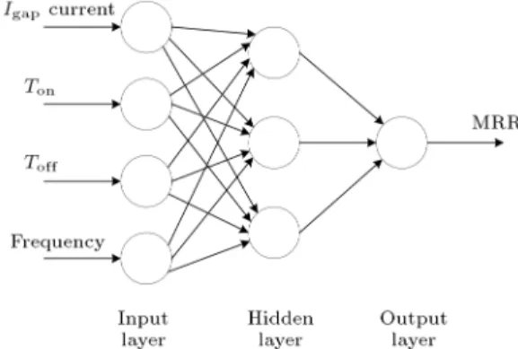
Figure 1. Architecture of the neural network model.

parameters in the dynamical system process. Research by using ANN to model the EDM process has also been reported in [2,10,12]. Generally, these papers explained well how to train the FFANN.

Figure 1 shows an example of a neural network structure, consisting of input, hidden and output layers in representing the machining knowledge of the EDM process. The rst layer is an input layer, where external information is received. The layer that is separated from the input layer by one or more intermediate layers is called the hidden layer. Each layer has a set of neurons or nodes, known as an information processing unit. The neurons in adjacent layers are usually fully connected by acyclic arcs from the left to the right layer [10].

According to the network structure, as given in Figure 1, decision variables in the modeling problem could be assigned as a set of input neurons such as the value of Igap, Ton, To and frequency (Fs). Response

variables are assigned as the set of output neurons; in this study, MRR is selected as the predicted output.

The functional relationship estimated by the FFANN for modeling purposes can be written as:

Y = f(x1; x2; ; xp); (1)

where (x1; x2; :::; xp) are p decision (independent)

vari-ables and Y is a response (dependent) variable [9]. So, for this case, Eq. (1) becomes:

MRR = f(Igap; Ton; To; Fs): (2)

A neuron with a single R-element input vector is shown in Figure 2. Here, the individual element inputs;

p1; p2; ; pR; (3)

are multiplied by weights:

w1;1; w1;2; ; w1;R; (4)

and the weighted values are fed to the summing junction. Their sum is simply W p, the dot product of the (single row) matrix, W , and the vector, p.

The neuron has a bias, b, which is summed with the weighted inputs to form the net input, n. This sum,

Figure 2. Single neuron [13].

Figure 3. Multiple neurons [13].

n, is the argument of the transfer function, f.

n = w1;1p1+ w1;2p2+ + w1;RpR+ b: (5)

This expression can be written in code as:

n = W p + b: (6)

Figure 2 shows single neuron with more details. Con-sidering networks with many neurons, and perhaps layers of many neurons, there is so much detail that the main thoughts tend to be lost. Thus, an abbreviated notation for an individual neuron must be devised. This notation of multiple neurons is shown in Figure 3. As seen in Figure 3, input vector p is represented by the solid dark vertical bar on the left. The dimensions of p are shown below the symbol, p, in Figure 3, as R 1. A capital letter, such as R in the previous sentence, is used when referring to the size of a vector. Thus, p is a vector of R input elements. These inputs post multiply the single-row, R-column matrix, W . As before, constant 1 enters the neuron as an input and is multiplied by a scalar bias, b. The net input to the transfer function, f, is n, the sum of the bias, b, and the product, Wp. This sum is passed

to the transfer function, f, to get the neuron's output, a, which, in this case, is scalar. Note that if there is more than one neuron, the network output will be a vector. A layer includes a combination of weights, the multiplication and summing operation, bias b, and transfer function, f.

Considering that the training of the neural net-work is based on a feed-forward back propagation algorithm, the following discussion is applied. Since the number of neurons found in the input and output layers

is known, the number of hidden layers is determined using a trial and error method [12]. Then, the error signals resulting from the dierence between the computed and actual values are back propagated from the output layer to the previous layers in order for them to update their weights. The weights are where FFANN saves the information over its acyclic arcs, and each arc has a weight. The weights are constantly varied while trying to optimize the relation between the inputs and the outputs. Determination of the number of hidden layers and the numbers of neurons for each hidden layer is performed by MATLAB. The number of iterations is entered by the user, and then the training starts. The training continues until the iterations reach the target level of error. The accuracy of the network is evaluated by the mean sum of the squared error (MSE) between the measured and predicted values of the training. The feedback from that processing is called the \average error" or \performance". Once the average error is below that of the required goal, the neural network stops training and is ready to be veried. In order to understand whether the FFANN is producing good predictions, test data that has never been presented to the network is used and the results are checked at a stage called the testing stage. In this paper, a training algorithm of EDM process parameters as a behavior model for FFANN is proposed.

3. Experimental data of EDM process

Experimental work for the EDM process is conducted using copper electrode and steel workpiece materi-als [11]. A BP200 hydrocarbon mineral oil is used as the dielectric uid. An \Open ushing" condition is applied to circulate the dielectric uid between the electrode and the workpiece.

The removed material for a given period is mea-sured in cubic millimetres per minute of a cylindrical form using the method detailed in Figure 4. During experimental work, some properties can be seen as follows:

Volume of material removal = D₄2 h; Electrode material: Copper;

Figure 4. Method used to measure the material removal rate.

Workpiece material: Steel; Dielectric uid: BP200:

Diameter D and height h were accurately measured using precision digital dial calipers. A cylindrical electrode with a diameter of 20 mm is used. The open gap voltage is set to 160 V. Several experiments were conducted at various Tonand Toin order to adjust the

sparking frequency, Fs, for optimum material removal

rate. The gap voltage, Vgap, drops until 25 V and,

at the same time, the gap current, Igap, rises up to a

selected constant value. The Igapis selected at 4A, 6A,

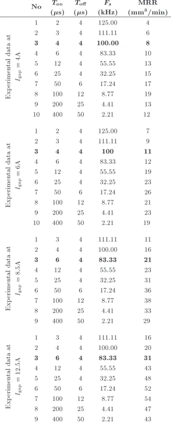
8.5A, 12.5A for nishing machining, and 18A, 25A, 36A and 50A for roughing machining. Experimental results of the MRR were recorded and presented in tabular form as shown in Tables 1 and 2. The bolded numbers are used for testing data and were never used in the training stage.

4. New training algorithm in feed forward articial neural network for EDM process model

A Feed Forward Articial Neural Network (FFANN) serves to process, learn, and predict information using layers of interconnected computational units. The quality of the network performance in such cases depends on its generalization ability, or the ability to recognize trends from the training data and employ what it has learned to make predictions on new test data. Nonetheless, FFANNs often perform poorly when applied to new cases dissimilar to those they have encountered, a aw possibly attributed to data anomalies that adversely aect the training process. Therefore, it is important to develop methods to improve a neural network's generalization ability, since the quality of future predictions from a comprehensive set of all possible data is the ultimate determinant of a network's prociency [14].

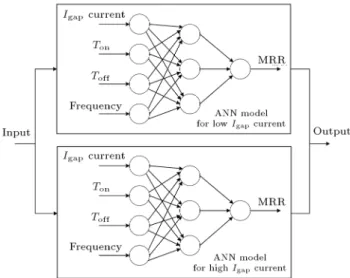
In principle, the method proposed in this re-search is an attempt to improve the performance of neural networks in predicting the MRR of the EDM process. From the experimental work, grouping data is performed based on the amount of current owing to the electrode-workpiece for roughing or nishing machining. Each group has its own neural network in accordance with a specied architecture. Therefore, this proposed method consists of two neural networks, one for modeling the EDM process for roughing ma-chining and the other for nishing mama-chining, as depicted in Figure 5.

The FFANN that will be used as a model is trained in the same way as reported earlier. At rst, all raw data is used to train the FFANN model and, then, the model is used to predict some

input-Table 1. Finishing machining parameters. No Ton

(s) To (s) Fs (kHz) MRR (mm3_/min)

Exp erimen tal data at Igap = 4A

1 2 4 125.00 4

2 3 4 111.11 6

3 4 4 100.00 8

4 6 4 83.33 10

5 12 4 55.55 13

6 25 4 32.25 15

7 50 6 17.24 17

8 100 12 8.77 19

9 200 25 4.41 13

10 400 50 2.21 12

Exp erimen tal data at Igap = 6A

1 2 4 125.00 7

2 3 4 111.11 9

3 4 4 100 11

4 6 4 83.33 12

5 12 4 55.55 19

6 25 4 32.25 23

7 50 6 17.24 26

8 100 12 8.77 21

9 200 25 4.41 23

10 400 50 2.21 19

Exp erimen tal data at Igap = 8: 5A

1 3 4 111.11 11

2 4 4 100.00 16

3 6 4 83.33 21

4 12 4 55.55 23

5 25 4 32.25 31

6 50 6 17.24 36

7 100 12 8.77 38

8 200 25 4.41 33

9 400 50 2.21 29

Exp erimen tal data at Igap = 12 :5A

1 3 4 111.11 16

2 4 4 100.00 20

3 6 4 83.33 31

4 12 4 55.55 43

5 25 4 32.25 48

6 50 6 17.24 52

7 100 12 8.77 54

8 200 25 4.41 47

9 400 50 2.21 43

output of the selected data. Then, data which are collected from the experiment are divided into two subsets, based on roughing or nishing machining. After the training step and applying the model to predict MRR, comparison between the two methods of training algorithm will be conducted.

Table 2. Experimental machining parameters. No Ton

(s) To

(s) Fs

(kHz)

MRR (mm3_/min)

Exp

erimen

tal

data

at

Igap

=

18A

1 4 4 100.00 16

2 6 4 83.33 42

3 12 4 55.55 54

4 25 4 32.25 68

5 50 6 17.24 79

6 100 12 8.77 86

7 200 25 4.41 72

8 400 50 2.21 65

Exp

erimen

tal

data

at

Igap

=

25A

1 4 4 100.00 46

2 6 4 83.33 60

3 12 4 55.55 81

4 25 4 32.25 99

5 50 6 17.24 126

6 100 12 8.77 126

7 200 25 4.41 110

8 400 50 2.21 90

Exp

erimen

tal

data

at

Igap

=

36A

1 6 4 83.33 72

2 12 4 55.55 111

3 25 4 32.25 137

4 50 6 17.24 181

5 100 12 8.77 175

6 200 25 4.41 151

7 400 50 2.21 141

Exp

erimen

tal

data

at

Igap

=

50A

1 6 4 83.33 82

2 12 4 55.55 143

3 25 4 32.25 170

4 50 6 17.24 218

5 100 12 8.77 250

6 200 25 4.41 221

7 400 50 2.21 200

Experiments were conducted using various Igap,

Ton, To and frequencies as variable parameters. The

amplitudes of the selected current are 4A, 6A, 8.5A, 12.5A, 18A, 25A, 36A and 50A. Based on the selected range of current amplitude, these ranges are divided into two segments, i.e., low for nishing and high for roughing Igap current. The purpose of this

segmenta-tion is to get a better MRR predicsegmenta-tion prole of the EDM process that is aected by two parameters, i.e. high and low Igap current. Based on [15], it has been

selected that four inputs, one hidden layer with three neurons and one output is the best architecture used to model the EDM pulsed power generator EDM process. This network was trained using a back propagation learning algorithm, since the combination of weights

Figure 5. A new architecture of the proposed neural network model.

which minimizes the error function is considered to be a solution of the learning problem. The time required is aected by selection of the learning rate and the learning rate was set to 0.57. After the neural network is trained for 15000 epoch, adaptation is stopped. As seen in Figure 5, there are two models of neural networks, one for modeling the EDM at low Igap current and the other for modeling the EDM at

high Igapcurrent.

5. Results and discussions

The rst step in using the neural network for modeling the EDM process is determination of the architecture and topology of the network to be used; for example, the number of hidden layers and the number of neurons in each layer in the networks. Based on [15], four inputs, one hidden layer with three neurons and one output is the chosen architecture used to model the EDM process.

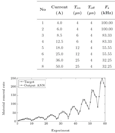
As stated earlier, during the training stage, all data was trained directly to the Feed Forward Ar-ticial Neural Network (FFANN) model. Training data is obtained from Table 1 (nishing) and Table 2 (roughing) except for each row 3, which will be used as testing data. The number of experimental data is 68. From these data, 8 are used in the testing stage. The remaining 60 data will be used during the training process. Figure 6 reveals experimental data, known as target and output data, known as output FFANN. In the gure, a circle is used to plot the target and a star is used for output FFANN. After the training process, the FFANN model follows the dynamical behavior of the EDM process, as shown in Figure 6.

Predicting MRR using the FFANN model can be conducted after the training process. Output FFANN as a predicted value for MRR will be compared to the

Table 3. Testing data and results using FFANN. No Current

(A)

Ton

(s) To

(s) Fs

(kHz)

MRR value (mm3_/min)

Prediction error Actual Predicted (%)

1 4.0 4 4 100.00 8 9.27 15.88

2 6.0 4 4 100.00 11 10.89 1.00

3 8.5 6 4 83.33 21 18.95 9.76

4 12.5 6 4 83.33 31 28.06 9.48

5 18.0 12 4 55.55 54 60.62 12.26

6 25.0 12 4 55.55 81 81.04 0.05

7 36.0 25 4 32.25 137 142.11 3.73

8 50.0 25 4 32.25 170 189.96 11.74

Figure 6. Comparisons between target and output neural networks using FFANN.

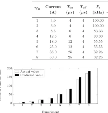
Figure 7. Comparison between actual and predicted values using FFANN.

experimental data. Figure 7 depicts the MRR which is obtained from the experiment, known as actual value, and the testing stage, known as predicted value. As mentioned previously, 8 data are used for the testing stage. From the gure, FFANN has good capability of predicting MRR, where the value of average error between predicted and actual values is 7.99%.

Table 3 represents the results in numerical value. From this table, the smallest dierences between actual and predicted values occurs when Igapcurrent is 25A,

Ton= 12 s, To= 4 s and Fs= 55:55 kHz.

A new modied algorithm for the training process is also presented in this paper by dividing it into two segments; low (nishing) and high (roughing) Igap

cur-Figure 8. Comparisons between target and output neural networks using ANFFANN.

rent. The proposed architecture is called A New Feed Forward Articial Neural Network (ANFFANN). Each of the networks uses the same architecture as shown in Figure 2. In this training algorithm, it is assumed that the capability of the neural network model is better, due to separation of the nishing and roughing process. For this proposed training algorithm, segmentation is introduced to make an agglomeration of the similarity of data. So, the generalization capabilities of the ANFFANN model are enhanced. Figure 8 plots two proles, which are known as the target and output of the ANFFANN model. As shown in the gure, the deviation of the output using the ANFFANN model is very small compared to the target. Once the new FFANN model is trained, the experimental data that had never been used during the training step will be applied to the testing stage. The results for predicting the MRR of the EDM process is presented in Figure 9. As seen in Figure 9, the new FFANN model has better capability in predicting the MRR of the EDM process. The numerical testing data and results are tabulated in Table 4, where the average error is found to be 5.07%.

6. Conclusion

In this paper, a Feed Forward Articial Neural Network (FFANN) algorithm has been applied to predict the

Table 4. Testing data and results using ANFFANN. No Current

(A)

Ton

(s) To

(s) Fs

(kHz)

MRR value (mm3_/min)

Prediction error Actual Predicted (%)

1 4.0 4 4 100.00 8 7.53 5.88

2 6.0 4 4 100.00 11 10.33 6.09

3 8.5 6 4 83.33 21 20.77 1.10

4 12.5 6 4 83.33 31 28.81 7.06

5 18.0 12 4 55.55 54 51.86 3.96

6 25.0 12 4 55.55 81 82.06 1.31

7 36.0 25 4 32.25 137 147.58 7.72

8 50.0 25 4 32.25 170 182.69 7.46

Figure 9. Comparison between actual and predicted values using ANFFANN.

MRR of the EDM process. The rst set of exper-imental data has been trained, where the selected unused data is used to predict the MRR. Another modied algorithm of the FFANN, called A New Feed Forward Articial Neural Network (ANFFANN), has been introduced later to predict the Material Removal Rate (MRR) by segmenting between the roughing and nishing process. In conclusion, the modied algorithm via segmentation has enhanced the accuracy of the FFANN model by 2%. The improved accuracy of the predicted Material Removal Rate (MRR) will inuence the development of the EDM machine feature. When the accuracy of the predicted MRR has been well received, the determination of machining time can be attached to the EDM machine. Determination of machining depth also will be improved. Moreover, backed by very fast FPGA technology, implementation of embedded FFANN will become true [16].

Acknowledgment

The authors wish to thank the Ministry of Science, Technology of Malaysia for their nancial support through the escience grant and UTM through GUP grant QJ130000.2645.08J82.

References

1. Benedict, G.F., Nontraditional Manufacturing Process, New York, Marcel Dekker (1987).

2. Mandal, D., Pal, S.K. and Saha, P. \Modelling of electrical discharge machining process using backprop-agation neural network and multi-objective optimiza-tion using non-dominating sorting genetic algorithm-II", Journal of Materials Processing Technology, 186, pp. 154-162 (2007).

3. Lin, C.L., Lin, J.L. and Ko, T.C. \Optimisation of the EDM process based on the orthogonal array with fuzzy logic and grey relational analysis method", International J. Adv. Manuf. Technol., 19, pp. 271-277 (2002).

4. Lin, J.L. and Lin, C.L. \The use of grey-fuzzy logic for the optimization of the manufacturing process", J. Mater. Process. Technol., 160, pp. 9-14 (2005). 5. Wang, K., Gelgele, H.L., Wang, Yi., Yuan, Q. and

Fang, M. \A hybrid intelligent method for modelling the EDM process", Int. J. Machine Tools Manuf., 43, pp. 995-999 (2003).

6. Su, J.C., Kao, J.Y. and Tarng, Y.S. \Optimisation of the electrical discharge machining process using a GA-based neural network", Int. J. Adv. Manuf. Technol., 24, pp. 81-90 (2004).

7. Kuriakose, S. and Shunmugam, M.S. \Multi-objective optimization of wireelectro discharge machining pro-cess by non-dominated sorting genetic algorithm", J. Mater. Process. Technol., 10, pp. 995-999 (2005). 8. Fenggou, C. and Dayong, Y. \The study of high

eciency and intelligent optimization system in EDM sinking process", J. Mater. Process. Technol., 149, pp. 83-87 (2004).

9. Ojha, K., Garg, R.K. and Sigh, K.K. \MRR im-provement in sinking electrical discharge machining: A review", Journal of Material & Characterization & Engineering, 9(8), pp. 709-739 (2010).

10. Tsai, K.M. and Wang, P.J. \Comparison of neural network models on material removal rate in electrical discharge machining", Journal of Material Processing Technology, 117 pp. 111-124 (2001).

11. Yahya, A. and Manning, C.D. \Determination of material removal rate of an electro-discharge machine using dimensional analysis", Journal of Physics D: Applied Physics, 37, pp. 1467-1471 (2004).

12. Assardeh, S. and Ghoreishi, M. \Neural-network-based modeling and optimization of the electro-discharge machining process", Int. J. Adv. Manuf. Technol., 39, pp. 488-500 (2008).

13. Multilayer Neural Network Architecture, Available from: http:// www.mathworks.com/ help/nnet /ug/ multilayer- neural-network- architecture. html 14. Thilagam, P.S., Pais, A.R., Chandrasekaran, K.

and Balakrishnan, N. \Generalization capability of articial neural network incorporated with pruning method", In Advanced Computing, Networking and Se-curity, pp. 171-178, Springer Berlin Heidelberg (2012). 15. Andromeda, T., Azli, Y. and Khamis, N.R. \Pre-dicting material removal rate of Electrical Discharge Machining (EDM) using articial neural network for low Igapcurrent", International Conference on

Exper-imental Mechanics (ICEM 2010), pp. 259-262 (2010). 16. Van Liempd, B., Herrera, D. and Figueroa, M. \An FPGA-based accelerator for analog VLSI articial neu-ral network emulation", 13th Euromicro Conference on Digital System Design: Architectures, Methods and Tools Lille, pp. 771-778 (2010).

Biographies

Trias Andromeda obtained a BS degree in Control Electronics and an MS degree in Electronics Signalling from Gadjah Mada University, Yogyakarta, Indonesia. He is currently lecturer in Diponegoro University, Semarang, Indonesia, and is pursuing his PhD de-gree in Electrical Engineering at Universiti Teknologi Malaysia. His research interests include Electrical Discharge Machining (EDM), power supply design, articial intelligence control and modeling.

Azli Yahya holds a BS degree in Electro Mechani-cal Power Systems and an MS degree in Electronic Production from Glamorgan University, UK, and a PhD degree from Loughborough University, UK, in Electronic and Electrical Engineering. He is currently

senior lecturer in Universiti Teknologi Malaysia. His areas of research include analog/digital circuit design, electrical discharge machining and power supply de-sign.

Nazriah Mahmud holds a degree in Biomedical Engineering from Universiti Teknologi Malaysia, where she is currently pursuing her PhD degree studies in the same subject. Her research interests include Electrical Discharge Machining (EDM), power supply design and micro-pitting.

Nor Hisham is a graduate of the University of Evansville, Indiana, USA, and holds a PhD degree in Electrical Engineering from Universiti Teknologi Malaysia, Malaysia, where he is senior lecturer in the Faculty of Electrical Engineering. He is also head of the Radar Laboratory in the Department of Radio Engineering and head of the Sonar Technology and Marine Instrumentation Research Group at Universiti Teknologi Malaysia.

Syahrullail Samion holds a PhD degree in Mechan-ical Engineering, specializing in Tribology in Metal Forming, Bio-lubricant and Fluid Mechanics, from Kagoshima University, Japan. He worked as a Me-chanical Engineer at Matsushita Audio Video (M) Ptd. Ltd. from May 2002 to January 2003, and is currently a lecturer in the Faculty of Mechanical Engineering at Universiti Teknologi Malaysia, majoring in Fluid Mechanics.

Ameruddin Baharom holds a BS degree in Elec-trical Engineering from Universiti Teknologi Malaysia and an MS degree in Digital Communication Systems from Loughborough University of Technology, UK. He is currently senior lecturer at Universiti Teknologi Malaysia. His research interests include digital com-munication, multiuser detection, and interference can-cellation.