CALCULATION OF BETA-DECAY RATES IN HEAVY DEFORMED NUCLEI AND IMPLICATIONS FOR THE ASTROPHYSICALr PROCESS
Thomas R. Shafer
A dissertation submitted to the faculty at the University of North Carolina at Chapel Hill in partial fulfillment of the requirements for the degree of Doctor of Philosophy in the Department of Physics and
Astronomy.
Chapel Hill 2016
Approved by:
Jonathan Engel
Charles Evans
Carla Fröhlich
Christian Iliadis
c
ABSTRACT
Thomas R. Shafer: Calculation of Beta-decay Rates in Heavy Deformed Nuclei and Implications for the Astrophysicalr Process
(Under the direction of Jonathan Engel)
The rapid neutron-capture process (r process) is responsible for synthesizing approximately half of the heavy elements in the solar system, but after decades of work the astrophysical site where it occurs is unknown. Because a very large number of heavy, neutron-rich nuclei are populated during ther process, theoretical efforts to locate ther-process site require a tremendous amount of nuclear physics input. However, most nuclei populated during ther process are very neutron-rich and unstable, and manyr-process nuclei cannot be studied experimentally. As a result, the basic properties of a large number of heavy, deformed, short-lived nuclei must be calculated with reliable nuclear models.
ACKNOWLEDGEMENTS
None of the work presented here would have been possible without the continuous guidance and assistance of my advisor, Jon Engel. I am tremendously grateful for the opportunity to study nuclear physics, but even more, I am grateful for his direction, insight, patience, and encouragement.
I am also indebted to the postdoctoral researchers with whom I have worked during my time at UNC, particularly Mika Mustonen and Matt Braby. I believe it was Mika who first suggested attempting to build what became the pnFAM, and I greatly enjoyed working closely with him these last few years to develop this method.
Many thanks are also due to my collaborators on this project, Carla Fröhlich, Gail McLaughlin, Matt Mumpower, and Rebecca Surman, who have provided astrophysical insight andr-process calculations for this work. I also gratefully acknowledge funding from the U.S. Department of Energy Topical Collaboration for Neutrinos and Nucleosynthesis in Hot and Dense Matter.
I especially thank the members of my committee: Charles Evans, Carla Fröhlich, Christian Iliadis, and John Wilkerson. I greatly appreciate the time and effort you have dedicated to this project.
I thank Nicolas Schunck, P. G. Reinhard, Markus Kortelainen, and Dong-Liang Fang for helpful notes, conversations, and computational programs during the course of this project. Also, my gratitude to Pedro Sarriguren for allowing me to reproduce his figures in Chapter 8 for a comparison between calculations.
Thanks to Derek Vermeulen and Laurie McNeil for supervising my experimental research project. I am tremendously grateful for the support and encouragement of my family and friends, including my parents, Rick and Liz; my brother and sister-in-law, Daniel and Brenda; the Godwins; my friends in Wilmington and from The Summit Church in the Raleigh-Durham area; and my friends from Archer Lodge Middle School. Life is so much better because of these people and many others.
TABLE OF CONTENTS
LIST OF TABLES . . . ix
LIST OF FIGURES . . . xi
LIST OF ABBREVIATIONS AND SYMBOLS . . . xiv
1 INTRODUCTION AND MOTIVATION . . . 1
1.1 The origin of the heavy elements . . . 1
1.2 Ther process . . . 2
1.2.1 Abundance features . . . 4
1.2.2 The search for ther-process site . . . 4
1.3 The importance ofβ decay inr-process calculations . . . 6
1.3.1 Outline of this work . . . 7
2 β DECAY IN NUCLEI . . . 8
2.1 Allowed and forbiddenβ decay . . . 9
2.2 The totalβ-decay half-life . . . 11
3 NUCLEAR SHAPE DEFORMATION . . . 13
3.1 Deformation and angular momentum symmetry breaking . . . 13
3.1.1 Angular momentum projection and the collective rotor model . . . 14
3.2 Matrix elements and transition strengths in the collective rotor model . . . 15
3.3 β-decay half-lives of axially-deformed nuclei . . . 17
4 DENSITY FUNCTIONAL THEORY AND THE LINEAR RESPONSE OF THE NUCLEUS . . . 18
4.1 The Skyrme energy-density functional . . . 20
4.2 Time-dependent DFT . . . 21
4.3 Linear response theory . . . 22
5.1 Mean field theory with pairing correlations: the HFB approximation . . . 25
5.1.1 HFB calculations with both protons and neutrons . . . 27
5.1.2 The ground state solver HFBTHO . . . 28
5.2 Overview of the finite amplitude method . . . 29
5.2.1 Differences between the charge-changing and like-particle FAM . . . 31
5.3 Solution of the pnFAM equations in the quasiparticle basis . . . 32
5.3.1 Strength functions, cross-terms, andβ-decay half-lives . . . 33
6 β DECAY OF ODD NUCLEI WITH THE PNFAM . . . 36
6.1 Ground states of odd nuclei and the equal filling approximation . . . 37
6.2 Excited states of odd nuclei . . . 39
6.2.1 The pnFAM equations for odd nuclei . . . 40
6.3 Interpretation of our results for odd nuclei . . . 42
7 β-DECAY HALF-LIVES OF RARE-EARTH ISOTOPES . . . 44
7.1 The rare-earthr-process nuclei . . . 44
7.2 Overview of the calculation . . . 45
7.3 Adjustments to and evaluation of ground state properties . . . 49
7.3.1 Adjustment of the pairing functional . . . 50
7.3.2 Calculated ground state properties . . . 52
7.3.3 Treatment of odd nuclei . . . 55
7.4 β-decay properties . . . 55
7.4.1 The time-odd functional . . . 56
7.4.2 The isoscalar proton-neutron pairing . . . 57
7.5 Evaluation of fits, results, and conclusions . . . 60
7.6 Consequences for rare-earthr-process nucleosynthesis . . . 66
8 β-DECAY HALF-LIVES OF ISOTOPES WITHA'80 . . . 69
8.1 Ground state properties . . . 70
8.1.2 Shape deformations and ground state pairing properties . . . 72
8.2 Excited states . . . 73
8.2.1 Fitting the proton-neutron isoscalar pairing . . . 74
8.3 Fit evaluation, results, and conclusions . . . 76
8.3.1 Half-lives ofA'80 nuclei . . . 76
8.3.2 Consequences for the weakr process . . . 80
9 CONCLUSIONS AND IMPLICATIONS FOR FUTUREr-PROCESS ANDβ-DECAY STUDIES 83 9.1 New calculations ofβ-decay half-lives of deformed nuclei . . . . 83
9.2 Consequences for ther process . . . 84
9.3 Future directions . . . 85
A DETAILED EXPRESSIONS FOR ALLOWED AND FIRST-FORBIDDENβ-DECAY RATES . . 87
A.1 Overview of the β-decay rate . . . 87
A.2 Allowed decay . . . 88
A.3 First-forbidden decay . . . 88
B NUCLEAR SHAPE DEFORMATION . . . 92
B.1 Nuclear matrix elements in the laboratory rest frame . . . 92
B.2 Reduced matrix elements, transition strengths, and cross terms . . . 94
C ADDITIONAL DETAILS INVOLVING THE DERIVATION OF THE PNFAM . . . 97
C.1 Derivation of the standard pnFAM equations . . . 97
C.1.1 Determination of the perturbed mean fieldsδH(ω) . . . 100
C.2 Modifications of the pnFAM equations for odd nuclei . . . 101
C.2.1 The perturbed mean fieldsδH(ω) in the pnFAM for odd nuclei . . . 103
LIST OF TABLES
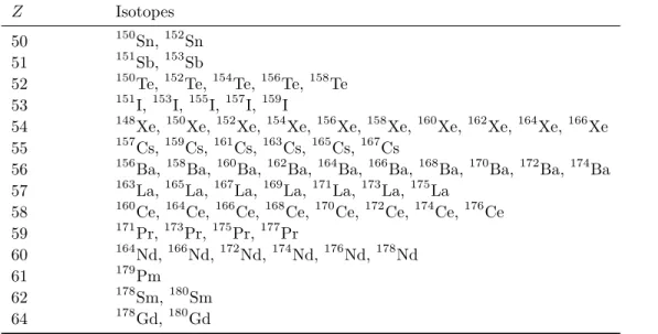
7.1 The seventy rare-earthr-process nuclei for which we computeβ-decay half-lives, including forty-five even-even nuclei and an additional twenty-five proton-odd nuclei. . . 45 7.2 Even-even nuclei used to fit the pairing strengthsVp andVn. The odd-even mass indicators
˜
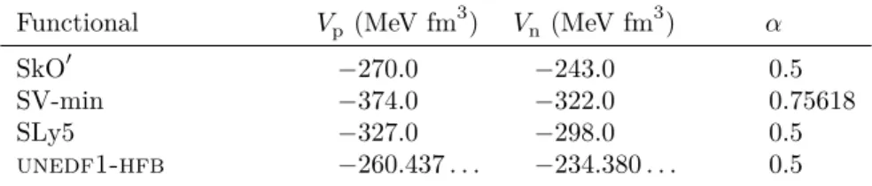
∆(3) are described in the text. . . 51 7.3 Values of the pairing strength and density dependence used in our rare-earth calculations. The
value of αfor SV-min, as well as all three pairing parameters forunedf1-hfb, were not changed. 51 7.4 Non-zero time-odd coupling constants used in our calculations. All couplings are in units of
MeV fm5 exceptC10s, which has units MeV fm 3
. The functional SkO0-Nd differs from SkO0 only in its value of the couplingC10s. . . 58 7.5 Isotopes used to fit the proton-neutron isoscalar pairing and, later, to evaluate our complete
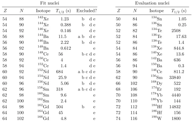
fitting procedure. The experimental half-lives were taken from Ref. [165]. The labels a–e in the “Excluded?” column note which isotopes were excluded from our pairing fits for the functionals (a) SkO0, (b) SkO0-Nd, (c) SV-min, (d) SLy5, and (e)unedf1-hfb. Isotopes were excluded when our calculated half-lives were shorter than experimental values and the proton-neutron isoscalar pairing was disabled. . . 59 7.6 Fitted proton-neutron isoscalar pairing strengths describing rare-earth nuclei. We have included
the dimensionless parametergpp=V0/V1= 2V0/(Vp+Vn), which measures the strength of theT = 0 pairing relative to itsT = 1 counterpart. That is, a valuegpp= 1 means theT = 0 pairing is the same strength as theT = 1 pairing. . . 60 7.7 Statistical measures of goodness-of-fit in the rare-earth region for both our entire set (Table 7.5)
and short-lived nuclei only. We have analyzed both the five EDFs used in this work and results from the global fit of Mölleret al [55]. The metricMr10= 10
Mr(described in the text and taken from Refs. [55, 125]) represents the mean deviation of a set of computed half-lives: Mr10= 1.0 implies a perfect fit (on average), andMr10= 2.0 implies a mean deviation by a factor 2. The standard deviation (σr10) and RMS error (Σ
10
r ) are defined similarly. On occasion we could not compute a reasonable half-life value and removed these isotopes from consideration (this is whyN changes for different EDFs). . . 62 8.1 The forty-five A'80 r-process nuclei studied in this work. Their locations on the nuclear
chart are also plotted in Fig. 8.2. . . 70 8.2 A'80 nuclei whose pairing properties entered into the proton and neutron pairing strength
adjustments. The experimental indicators ˜∆(3) (7.7) are computed using data from the 2012 Atomic Mass Evaluation [157] as described in Chapter 7. Nuclei withZ = 28 orN = 50 have
˜
∆(3) set to zero by hand. . . 71 8.3 A'80 nuclei whose half-lives were taken as inputs to adjust the proton-neutron isoscalar
pairing. Isotopes in the left column were used to determine the pairing strength for non-magic nuclei, and isotopes in the right column were used to determine the pairing strengths for nuclei with at least one closed shell. The experimental half-lives were taken from the ENSDF [168]. 74 8.4 Fitted proton-neutron isoscalar pairing strengthsV0 for open-shell and closed-shell nuclei as
LIST OF FIGURES
1.1 The nuclear landscape. Nuclei with experimentally-measured half-lives are shaded light, and “stable” nuclei with half-livesT1/2>109 yr are shaded dark. TheN = 50, 82, and 126 and
Z = 28, 50, and 82 shell closures are marked with solid lines. The r-process nuclei with
A'80 (blue circles) andA'160 (red circles) studied in this work are also highlighted past the neutron-rich edge of the experimental measurements. The experimental data are from nubase2012[6]. . . 2 5.1 Schematic demonstration of the contourC used to compute the totalβ-decay half-life. The
contour is defined in the complexω plane such that it includes all the poles (marked with red crosses) that are energetically allowed to contribute. This figure demonstrates to behavior of both the real and imaginary parts of the strength functionS(ω) folded with an analytic approximation to the phase space factorf(ω) as described in Ref. [61]. Reprinted figure with permission from M. T. Mustonen, T. Shafer, Z. Zenginerler, and J. Engel, Phys. Rev. C90, 024308 (2014) [61]. Copyright 2014 by the American Physical Society. . . 35
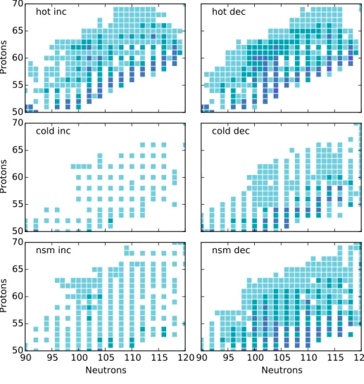
7.1 Sensitivity ofr-process abundances to increases (“inc”) and decreases (“dec”) of individual rare-earthβ-decay rates by a factor of 5. The most darkly shaded nuclei produced the largest effects. The figure is courtesy of M. Mumpower [62] and includes results for threer-process trajectories: a hotr process, a coldr process, and a neutron star merger. . . 46
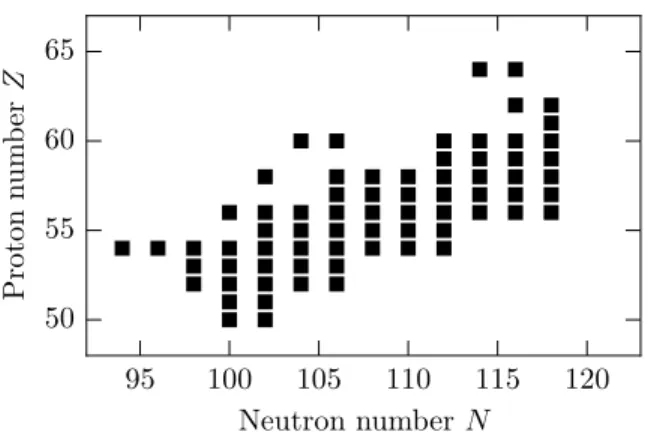
7.2 The locations on the nuclear chart (cf. Fig. 1.1) of the seventy rare-earth nuclei listed in Table 7.1. 47
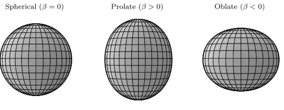
7.3 Schematic demonstration of the three classes of nuclear shapes allowed in our calculations as a function of the quadrupole deformation parameterβ (Eq. (7.9)). . . 52
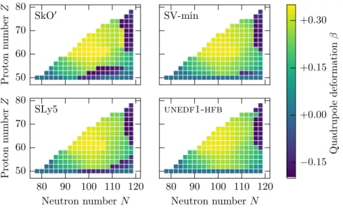
7.4 Ground state quadrupole deformationsβ obtained withhfbthofor even-even nuclei using the energy-density functionals (a) SkO0, (b) SV-min, (c) SLy5, and (d)unedf1-hfb. A prolate deformation maximum is clearly visible withZ≈60 and 100≤N≤110. . . 53
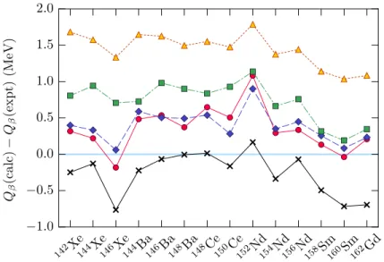
7.5 Difference between calculated and experimentalQβ values for a selection of rare-earth nuclei using the Skyrme functionals SkO0 (red circles), SV-min (blue diamonds), SLy5 (green squares), and unedf1-hfb (yellow triangles). The Q values of Möller et al. [160] (crosses) have been included for comparison. Experimental values are taken from the 2012 Atomic Mass Evaluation [157]. . . 55
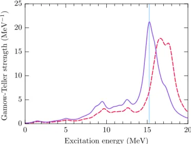
7.6 Demonstration of the effect of changing the coupling constantC10s on the Gamow-Teller giant resonance in150Pm. The strength function obtained with the functional SkO0, adjusted to the Gamow-Teller giant resonance in208Bi, is plotted with a red dashed line and misses the experimental value [164] (vertical line) by a few MeV. The SkO0 strength function adjusted to reproduce this resonance, called SkO0-Nd, is plotted as a solid line and shows slightly increased low-energy transition strength. . . 57
7.7 Evaluation of our adjustments through comparison between our calculated half-lives and experimental values for the nuclei in Table 7.5. By plotting the ratioT1/2(calc)/T1/2(expt), our best calculations lie along the solid line with the ratio equal to 1, and nuclei with short experimental half-lives are generally better-reproduced. Filled symbols represent nuclei in the left column of Table 7.5, and open symbols represent the nuclei in the right column (i.e., not even considered in the proton-neutron pairing fit). The shaded area represents a deviation of
7.8 Calculated half-lives for the seventy rare-earth nuclei in Table 7.1. The various markers correspond to SkO0 (red circles), SkO0-Nd (purple triangles), SV-min (blue diamonds), SLy5 (green squares), andunedf1-hfb(orange triangles). . . 63 7.9 Evolution of (a)Qvalues and (b) half-lives for neutron-rich Xe isotopes. Panel (a) includes
Q values calculated with the finite-range droplet model (FRDM) of Möller et al. [160] for comparison. In panel (b) we have also included half-lives calculated with SkO0-Nd, which share the sameQvalues as SkO0. . . 64 7.10 Comparison of our results applying the EDFs SkO0 (red circles), SkO0-Nd (purple triangles),
and SV-min (blue diamonds) with those of Mölleret al. [55] (crosses) for the same nuclei as Fig. 7.8. Vertical lines separate isotopic chains, which are ordered with increasingZ as in the previous figure. . . 65 7.11 Multipole decomposition of the β-decay transition strength for all seventyr-process nuclei in
Table 7.1, in ascending order of Z andN. Allowed (1+) decays dominate as expected, but the first-forbidden transitions (0−, 1−, and 2−) comprise a significant fraction of theβ strength. (Fermi (0+)β decay is neglected since these transitions occur at very high excitation energies.) 66 7.12 First-forbidden contributions to theβ-decay rate for the functional SV-min. The results are
plotted as a percentage, i.e., “50%” means that the first-forbidden transitions make up 50% of theβ-decay rate. . . 67 7.13 Calculated r-process abundances, using the same trajectories as Fig. 7.1, that incorporate
theβ-decay half-lives calculated in this work. The solid black line is the baseline abundance distribution obtained with theβ-decay calculations of Mölleret al. [55]. Figure courtesy of M. Mumpower [62]. . . 68 8.1 Sensitivity study in the A '80 region similar to that described in Ref. [141], courtesy of
R. Surman [62]. Rates were varied by a factor of 10 to obtain this figure, and nuclei are shaded more darkly with increasing importance to ther process. Stable isotopes are marked by crosses, and the grey line denotes the boundary between measured and not-measuredβ-decay half-lives. 69 8.2 Locations of ther-process nuclei in Table 8.1 on the nuclear chart (cf. Fig. 1.1). TheZ= 28
andN = 50 shell closures are also highlighted. . . 70 8.3 Quadrupole deformationsβ of nuclei in theA'80 region. . . 73 8.4 Dependence of our calculated half-lives on the isoscalar pairing strength V0 for open-shell
(solid lines) and semi-magic (dashed lines) nuclei listed in Table 8.3. These half-lives are plotted as the ratioT1/2(calc)/T1/2(expt), so a value 1.0 indicates perfect agreement between calculation and experiment. The curves were obtained by interpolating between logarithms of our calculated values T1/2(calc) using splines before plotting the values 10
log10T1/2(interp). The grey shaded area highlights the region in which our calculations agree with experimental results within a factor of 2. . . 75 8.5 Evaluation of our SV-min adjustment (top) compared to the result of Mölleret al. [55] (bottom)
8.6 β-decay half-life chains for Ge, Se, and Kr, with our calculations (stars) plotted alongside those reproduced from Ref. [125] (“[Sa15] prolate/oblate”). All experimental values, including those from systematics (“sys.”), are reproduced from Ref. [125]. Adapted with permission from Ref. [125]. Copyrighted by the American Physical Society. . . 78 8.7 Calculated half-lives in this work for the forty-fiveA'80r-process nuclei in Table 8.1 (red
circles) compared with corresponding values from Mölleret al. [55] (blue crosses). . . . 78 8.8 Contributions of the allowed (1+) and first-forbidden (0−, 1−, 2−) transitions to the total
β-decay rate for the r-process nuclei in Fig. 8.7. Isotopic chains are separated by dashed vertical lines and are ordered as in Fig. 8.7. . . 79 8.9 Total first-forbidden contribution to the β-decay rate as a function of proton and neutron
number. The copper (Z = 29) and zinc (Z = 30) isotopes, as well as89Ge, stand out as the only isotopes with significant forbidden contributions. . . 80 8.10 Weakr-process abundances computed with three sets ofA'80β-decay half-lives: those from
this work (red), Mölleret al. [55] (purple), and REACLIB [56] (blue). Figure courtesy of R. Surman [62]. . . 81 8.11 Impact of changes to theβ-decay half-lives of individual elements on weakr-process abundances,
LIST OF ABBREVIATIONS AND SYMBOLS
A Number of nucleons in the nucleus
DFT Density functional theory
EDF Energy-density functional
EFA Equal-filling approximation
FAM Finite amplitude method
HFB Hartree-Fock-Bogoliubov
N Number of neutrons in the nucleus
pnFAM Proton-neutron finite amplitude method
QRPA Quasiparticle random-phase approximation
REE Rare-earth element
RPA Random-phase approximation
TDDFT Time-dependent density functional theory
TDHFB Time-dependent Hartree-Fock-Bogoliubov
CHAPTER 1: INTRODUCTION AND MOTIVATION
Nucleosynthesis, the set of processes responsible for forming the atomic nuclei in matter, is a fundamentally important research area; it has also proven tremendously challenging to understand in full. Because nucleosynthesis occurs in and near stars, its study is interdisciplinary: beginning with the seminal work of Burbidgeet al. [1] and Cameron [2] nearly sixty years ago, efforts to understand these stellar processes have required both nuclear physics and astrophysics—theoretical calculations alongside laboratory experimentation and astronomical observation.
Among the processes required to produce the elements in nature [1, 2], those responsible for nuclei heavier than iron have proven especially challenging to unravel. In this work we provide new nuclear physics calculations—β-decay half-lives of heavy, deformed, neutron-rich nuclei—in an effort to better understand the astrophysical origins of these heavy elements. In particular, we examine nucleosynthesis via the rapid neutron-capture process (r process), which forms approximately half of the nuclei heavier than iron (see, e.g., the reviews [3–5]). In this introductory chapter we summarize the basics ofr-process nucleosynthesis and the importance of improved β-decay half-lives (and improved nuclear physics input in general) to theoretical r-process studies.
Section 1.1: The origin of the heavy elements
Since the 1950s [1, 2] it has been understood that nuclei are formed in and near stars by a variety of processes. This nuclear material can subsequently be expelled in a variety of catastrophic processes including supernovae [2]. However, even the most massive stars can only produce nuclei as heavy as Fe (withZ = 26 protons) in their cores; the formation of heavier nuclei is prohibited by both nuclear and astrophysical considerations (see Ref. [3] and references therein). The bulk of the nuclear material (and there are of course many nuclei heavier than Fe, cf. Fig. 1.1) must be made by other means.
0 60 120 180 Number of neutrons
0 60 120
N
u
m
b
er
o
f
p
ro
to
n
s
Figure 1.1: The nuclear landscape. Nuclei with experimentally-measured half-lives are shaded light, and “stable” nuclei with half-livesT1/2>109 yr are shaded dark. TheN = 50, 82, and 126 andZ= 28, 50, and 82 shell closures are marked with solid lines. Ther-process nuclei withA'80 (blue circles) andA'160 (red circles) studied in this work are also highlighted past the neutron-rich edge of the experimental measurements. The experimental data are from nubase2012[6].
and another new process, theνpprocess [10–12] (which leverages the large neutrino fluxes in core-collapse supernovae (CCSNe) to create additional neutrons), has been introduced and suggested to be a candidate LEPP. These new processes do not change the overall picture of abundances dominated by neutron capture.
Focusing on then-capture processes specifically, thes process (which operates through neutron capture that occurs less frequently thanβ decay, on a time scale of 10–100 years [2]) forms neutron-rich nuclei near the valley of β stability. Ther process operates on much shorter time scales (τ ∼ 1 s) and is necessary for producing heavier neutron-rich nuclei that cannot be made in thes process [1, 2]. Many nuclei can of course be formed in varying proportions by both processes (see Ref. [13] and references therein), though a few elements are understood to be nearly pures- orr-elements (e.g., Eu is anr-element [14]).
The s process is the better understood n-capture process (see the review [15] as well as Ref. [3] and references therein), and calculateds-process abundances (e.g., Ref. [14]) are typically used to obtainr-process residuals via “solar minuss-process” calculations [16, 17] (also see Refs. [3, 4, 13] and references therein). Ther process, on the other hand, has many important questions still unanswered [4], not the least of which is its astrophysical site.
Section 1.2: The r process
“canonical” or “hot”r process (described in many places, see, e.g., Refs. [3, 4, 18]), neutron capture takes place on very short time scales, much shorter thanβ decay (usually writtenτn τβ), as a result of the large number of free neutrons. Lighter seed nuclei (e.g., Fe isotopes) that are produced during ther process and then exposed to this neutron flux will quickly capture neutrons and form extremely neutron-rich isotopes.
Depending on the conditions, these heavy isotopes may be so neutron-rich as to approach the neutron drip line (at which point no additional neutrons may be bound to the nucleus). At the high temperatures described in Ref. [1], however, the r process can reach a statistical equilibrium between neutron capture and its reverse reaction, photo-dissociation. This (n, γ)(γ, n) equilibrium ensures that somewhat lighter nuclei are populated instead, as high-energy photons remove the most weakly-bound neutrons from the most neutron-rich isotopes.
After a long time relative to then-capture time scaleτn, ther process will have formed many neutron-rich,
β-unstable isotopes. Eventually (on theβ-decay time scale,∼1–1000 ms) these unstable isotopes will begin to decay, gaining relative stability by moving towards the valley ofβstability by one unit: (Z, N)→(Z+1, N−1). The decay products will then repeat the capture-and-decay process as long as free neutrons are still available. In this way the r process forms very short-lived, neutron-rich isotopes of the heavy elements (Z 26) very quickly, over just a few seconds. The most neutron-rich scenarios (for example, that of a neutron star merger [4]) can form such heavy nuclei that fission plays a role as well. This can lead to fission cycling, in which fission products themselves experience the r process, perhaps eventually leading to additional fissions.
Eventually, the r process begins to wind down as neutron capture and photo-dissociation fall out of equilibrium [18]. As this happens,β decay begins to take place on approximately the same time scale as (or faster than) neutron capture and photo-dissociation—the latter processes occur less frequently either due to lack of neutrons or lowered temperatures [19]. The β-unstable material formed during the (n, γ)(γ, n) equilibrium then decays towards stability, andβ decay competes with neutron capture and photo-dissociation for some time. This competition can affect final abundance patterns beforen-capture and photo-dissociation freeze out completely, leaving the material toβ decay to stability (see, e.g., Ref. [20]).
1.2.1: Abundance features
The fast neutron capture described above is responsible for the hallmarkr-process abundance features: sizable increases in the amounts of nuclear material with the mass numbersA= 80, 130, and 195 [1, 2]. These features are important as anr-process signature, and theoretical calculations must be able to reproduce them.
The large abundances at these mass numbers are explained by filled neutron shells in a nuclear shell model, corresponding to the “magic” numbersN= 50, 82, and 126 [22] (also see Refs. [1, 2] and additional references therein). Closed neutron shells have reducedn-capture cross-sections, and, if captured, an additional neutron is not very bound [22]. These nuclei also tend to have longβ-decay half-lives [18] and are often calledr-process “waiting points.” As nuclear material moves up the nuclear chart to larger values ofZ during ther process, reducedn-capture cross-sections for closed-shell nuclei act to trap nuclear material. (In fact thes process forms similar features at the slightly larger mass numbersA'90, 138, and 208 [1, 2].) These abundance peaks are formed during the main phase of ther process, i.e., during the (n, γ)(γ, n) equilibrium if one persists.
In addition to the three primary r-process abundance peaks, there is also a fourth, somewhat smaller, peak in the region of the rare-earth elements (REEs) withA'165. Understanding the formation of this REE abundance peak has been a challenge, as summarized in Refs. [18, 19] and references therein: Burbidge et al. [1] suggested the REE peak was formed during ther process as a consequence of nuclear deformation; and Cameron [2] hypothesized it was due to fission, though this was later deemed unlikely [23]. (Fission seems to have re-emerged as a potential driver [24] of, or at least as a contributor [19] to, the REE peak.)
Surman and Engel [18] demonstrated nicely that the REE peak is, in fact, caused by a local maximum in the nuclear shape deformation, but not during the main phase of ther process. Rather, at least for a hotr process, the peak is only formed at late times after neutron capture and photo-dissociation have fallen out of equilibrium; changes in nuclear shape deformation weakly mimic a shell closure. Refs. [19, 20] also found this effect, and Ref. [20] further demonstrated that the REE peak could also be formed during a coldr process without a prolonged (n, γ)(γ, n) equilibrium, albeit via a slightly different mechanism. Because of the unique dynamics that govern the formation of the REE peak, its formation can provide additional insight into ther process [19, 20].
1.2.2: The search for the r-process site
The uncertainties in nuclear physics input stem from both the neutron richness of the nuclei involved in ther process and the sheer number of nuclei that are involved to make the heavy elements. Because ther process forms so many nuclei, accurate and precise abundance calculations for different astrophysical sites require nuclear physics input for a tremendous number of nuclei including masses, reaction rates, and fission barriers [25] (see also a summary in Ref. [4]). The neutron-richness of r-process nuclei also means that few-to-none of these key properties can be measured in current-generation experiments for the most neutron-rich nuclei [4].
As a result, astrophysical calculations must rely on nuclear physics input derived from separate nuclear physics calculations. These calculations of nuclear properties have their own uncertainties that are potentially compounded by extrapolation to regions of high neutron-excess (see Ref. [3] and references therein). Recent work by Mumpower and collaborators has demonstrated that typical uncertainties in nuclear masses [25] as well as neutron-capture andβ-decay rates [26] remain a serious hindrance to precise predictions ofr-process abundances (see also Ref. [27] and references therein).
Setting aside the nuclear physics component, the astrophysical picture is even less clear [4]. It now seems likely that there is a distinction betweenr-process scenarios that form the elements above and below
A'140 [28], and these processes have been named the “main” and “weak”r processes, respectively. This classification may not be set in stone (see, e.g., the reviews [5, 13] and references therein), but is supported by (1) the “robust” nature of observed mainr-process abundances and (2) the scatter in weak r-process abundances (see, e.g., the reviews [5, 13, 29–31]). It has also been demonstrated over time that observational data can described by a phenomenological two- or three-componentr-process model [32–39].
However, the challenge of identifying the astrophysical sites corresponding to the weak and mainr process remains. The neutrino-driven wind (NDW) of a core-collapse supernova has long been investigated as a potentialr-process site, but modeling these supernovae is extremely complicated (see, e.g., the review [40]). As increasingly-sophisticated models become available, the NDW no longer appears to be a strong candidate for a mainr process and in fact seems more likely to be proton-rich than neutron-rich (see, e.g., the recent review [31] and references therein).
the picture to explain earlyr-process abundances.
Indeed, many astrophysical scenarios still seem possible. Combinations of core-collapse supernovae, magnetorotational core-collapse supernovae, and neutron star mergers can produce solar abundances [49]; neutron star mergers and magnetorotational supernovae can similarly describe galactic Eu abundances [50]; and perhaps magnetorotational core-collapse supernovae can explain both the main and weakr processes [48]. Disentangling this knot will clearly require the continued effort of astrophysics and nuclear physics working in concert.
Section 1.3: The importance of β decay inr-process calculations
As discussed above,r-process studies require a tremendous amount of nuclear physics input, and many different nuclear inputs play a role. β decay in particular plays a key role by determining (1) how quickly nuclear material moves through the waiting points and (2) final abundances distributions as material decays back towards stability. This second effect has been shown to be particularly important in the formation of the REE abundance peak, where the interplay ofβ decay and neutron capture after the (n, γ)(γ, n) equilibrium has ended builds up the peak [18, 20]. This suggests that accurate modeling of β decay is particularly important for rare-earth nuclei, although recent neutron star merger calculations indicate the REE peak is actually quite robust for differentβ-decay half-life calculations [42].
As with other critical r-process inputs, it is important to improve our understanding of theβ decay of neutron-rich nuclei. The uncertainties present in typical calculations remain large enough to seriously affect resulting uncertainties inr-process calculations [26, 27], and as the reach ofβ-decay experiments has increased it has been found that many theoretical calculations predict too-longβ-decay half-lives for nuclei near closed shells. Changes in these half-lives modify computedr-process abundances (see, e.g., Refs. [51–53] and references therein). For example, speeding up β-decay half-lives near N = 126 has been shown to affect theA= 195r-process peak in neutron star merger calculations and bring calculations closer to solar observations [24], and Eichleret al. [53] have found similar effects when increasingβ-decay rates for nuclei with
Z >80. Caballeroet al. [51] have also studied the effect of reducedβ-decay half-lives near magic numbers, while Madurgaet al. [54] have measured shorter half-lives for Zn and Ga isotopes than those predicted by Mölleret al [55] and produced new calculations that yield significant effects onr-process abundances for nuclei heavier thanA= 140.
Perhaps the standard set ofβ-decay half-lives in use today is that of Mölleret al. [55] from more than a decade ago, while the REACLIB database1 [56] still includesβ-decay half-lives that are thirty years old [57]. In addition to many recent smaller-scale β-decay calculations, however, new large-scale calculations are
1
beginning to become available: Marketinet al. [58, 59] have recently computed the half-lives of more than 5,400 neutron-rich nuclei (although these calculations do not treat nuclear shape deformation), and Mustonen and Engel [60] have computed half-lives of nearly 1,400 even-even nuclei using the method detailed and applied in following chapters.
In this work we present newβ-decay half-lives in both the REE peak region (A'165) and the weak r-process region (A'80), shown in Fig. 1.1. Our calculations are both self-consistent (ground states and β
transitions are calculated with the same nuclear interaction) and microscopic (nucleons are the only degrees of freedom). The microscopic nature of these calculations is important to increase confidence in predictions for very neutron-rich nuclei (see, e.g., the discussion in Ref. [4]). Our calculations incorporate both pairing correlations and nuclear shape deformation, but our method (called the proton neutron finite amplitude method, or pnFAM [61]) remains efficient enough to allowβ-decay calculations across the entire nuclear chart as presented in Ref. [60].
We have calculated rare-earth β-decay half-lives to (1) compare our new calculations to the standard ones of Mölleret al. [55] and (2) examine the consequences for ther process in the REE peak region. The overall speed ofβ decays in the rare-earth region, for example, can determine the overall abundance in the rare-earth peak [62]. Unlike the REE peak,A'80 abundances appear to be formed by a variety of processes (see, e.g., Refs. [5, 31] and references therein). With the new calculations presented here, we examine the impact of
β-decay half-lives on r-process calculations in this lighter mass region. In this way we hope to shed light on ther-process contribution to these abundances.
In this work we also present an extension of the pnFAM that enables the calculation ofβ-decay half-lives for both singly and doubly odd nuclei (when referring to both classes collectively, we simply call them ‘odd’ nuclei). This extension is incorporated into both ourA'165 and A'80 calculations, and will allow the inclusion of odd nuclei in future microscopic calculations across the nuclear chart without serious difficulty.
1.3.1: Outline of this work
CHAPTER 2: β DECAY IN NUCLEI
In this chapter we briefly review nuclear β decay and demonstrate how we calculate half-lives (or, equivalently, decay rates) from nuclear matrix elements of the weak interaction. β decay is unique among typical nuclear radiation (α, β, and γ), a product of the weak nuclear force [63], and provided the first demonstration of a fundamental interaction that does not exhibit mirror (or, parity) symmetry. Besides the obvious applications of β decay to nuclear radioactivity, its discovery also led to the proposition and subsequent discovery of the (nearly) massless neutrino [63, 64] which remains the subject of large-scale experimental efforts.
The simplest example ofβ decay is that of a free neutron [63–65], with a half-life of approximately 10 minutes [66], in which the neutron decays into a proton, electron, and antineutrino (β− decay):
n→p+e−+ ¯νe. (2.1)
The decay is energetically possible since the neutron is more massive than the proton-electron-neutrino combination by approximately 782 keV/c2[66]. Alongsideβ−decay are two relatedβ-decay processes: proton decay (β+decay)
p→n+e++νe, (2.2)
and electron capture
e−+p→n+νe. (2.3)
Neither of the decays (2.2) or (2.3) are allowed for free particles at rest since the proton mass (and the combined mass of the proton and electron in Eq. (2.3)) is less than that of the neutron. Inside the nucleus, however, the interactions among the nucleons that make up the nuclear binding energy significantly affect the stability of the constituent nucleons. These interactions allow nuclearβ+ decay and electron capture to occur in some cases and significantly affect β-decay half-lives in general. In many nuclei near the “valley of stability” (dark shaded squares in Fig. 1.1), for example,β− decay is either energetically impossible [63] or strongly suppressed. In regions with large neutron excesses (as inr-process nuclei), the nuclear half-life may fall well below that of the free neutron, into the millisecond range. And on the proton-rich side of the
decay in this work since ther-process abundances of interest depend on the half-lives of neutron rich nuclei. The nuclear equivalent of the β decay of a free neutron (2.1) is the process
(Z, N)→(Z+ 1, N−1) +e−+ ¯νe, (2.4)
i.e. one of theN neutrons in the nucleus decays, resulting in a nucleus withZ+ 1 protons andN−1 neutrons. The energy balance in theβ-decay process (2.4) is written1 [64]
Mi(Z, N) =Mf(Z+ 1, N−1) +me+Q, (2.5)
where Mi andMf are the initial and final nuclear masses, and meis the electron mass. In the limit of very large initial and final nuclear masses and zero neutrino mass (both very good approximations inβ decay [65]), theQvalue is the kinetic given to the emitted leptons [64]. Values forM(Z, N) must either be taken from experiment or calculated. Calculations must account for both the masses of the nucleons themselves and the nuclear binding energy.
For decays to the ground state of the daughter (final) nucleus, the Qvalue is given the symbolQβ. To calculate the totalβ-decay half-life we must also account for decays to all the energetically allowed excited states in the daughter nucleus. These states have excitation energiesEx with respect to the ground state of the daughter, and theQvalues for these decays are smaller than Qβ by the excitation energy [64]:
Qx=Qβ−Ex. (2.6)
Section 2.1: Allowed and forbidden β decay
Nuclear β decay is often described as being either “allowed” or “forbidden,” with these classifications being named according to the relative rarity of decay—forbidden decays occur much less often than allowed decays. This classification arises naturally from the matrix elements of the weak nuclear interaction, which can be demonstrated by considering a schematic version ofβ decay. In this section, we follow the presentation of Refs. [64, 67].
Because the weak nuclear interaction is, in fact, weak compared to the strong nuclear and Coulomb interactions inside the nucleus, a first-order perturbation theory treatment of its effect on the nucleus is acceptable and results in Fermi’s “golden rule” [63, 64, 67] for the decay rateλ(the probability of a nucleus
1
to decay per unit time [63]):
λ= 2π
~
Mf i
2
ρ(Ef). (2.7)
The decay rate is inversely related to the half-life: λ= ln 2/T1/2. Up to some constants, the decay rate is the product of (1) the square of a matrix elementMf i, which describes the β-decay the nucleus, and (2) a phase space factorρ(Ef), which counts the number of final states the emitted leptons can decay into as a function of their total energyEf.
The matrix elementMf i is the amplitude for a nucleus in the state|iitoβ decay to the daughter state
|fias in Eq. (2.5) and can be written approximately as [64, 67]
Mf i= Z
Ψ∗f(r)ϕ
∗
e(r)ϕ
∗
ν(r) ˆV(r) Ψi(r) d 3
r, (2.8)
where Ψi and Ψf are the initial- and final-state nucleon wave functions. The emitted leptons are described by plane waves:2
ϕe(r)ϕν(r)∝e iq·r
, (2.9)
withq≡pe+pν their total momentum. The overlap of the lepton wave functions with the nucleus is quite small [64]—the nuclear radius is typically approximated byR≈1.2A1/3fm [67], soR≈5.6 fm whenA= 100. As a result, a Q= 1 MeV decay givesqR≈0.04, and a 10 MeV decay hasqR≈0.3. Expanding the lepton wave functions in powers ofq·rgives a series of matrix elements,
Mf i= Z
Ψ∗f(r) [1−iq·r−. . .] ˆVweak(r) Ψ
∗
i(r) dr =Mf ia +M
ff f i+. . . ,
(2.10)
that involve only the nuclear wave functions, the weak interaction, and powers ofq·r. Since the decay rate depends onM2, the contribution of the second term in Eq. (2.10) is reduced by a factor between 10 and 1000 (approximately) relative to the first, all else being equal. The first term describes allowed decays, and the
second describes “first-forbidden” decays.
In allowed β decay the leptons are emitted without orbital angular momentum, and the parity of the daughter nucleus is the same as the parent (πi=πf, orπ= +1) [64]. Despite not possessing orbital angular momentum, the leptons may still carry nonzerototal angular momentumJ depending on whether the lepton spins are anti-aligned (J = 0) or aligned (J = 1). Allowed transitions must correspondingly change the
2
angular momentum of the nucleus by zero or one unit to conserve angular momentum—“Fermi” transitions do not change the angular momentum of the nucleus (∆J = 0) or its parity (π= +1), but their “Gamow-Teller” counterparts can change the total angular momentum by zero or one unit without changing the parity of the nuclear wave function: ∆Jπ= 0+ or 1+.
First-forbidden decays are more complicated, but they follow the general rules outlined above. The lepton spins still either align or anti-align, but in these decays the leptons carry offL= 1 unit of angular momentum as well, changing the parity of the nuclear wave function. The total angular momentum carried by the leptons is then the vector sum of their spin angular momentum (S = 0 or 1) and orbital angular momentum (L= 1), and it can take the valuesJπ= 0−, 1−, or 2−.
If we continued with this expansion, each additional term would be reduced in magnitude by approximately
qR, increase the lepton orbital angular momentum by 1 unit, and flip the parity of the nucleus again. Such transitions are called second, third, and fourth forbidden, etc. SinceqRis fairly small, the positive-parity allowed transitions will usually provide the dominant contribution to the decay rate. There are regions of the nuclear chart, however, where eitherqRis not small or the allowed transitions are suppressed enough (e.g., transitions between certain major shells in a nuclear shell model [70]) for first-forbidden decays to be non-negligible. Our r-process calculations involve both moderately neutron-rich (A ' 80) and very neutron-rich (A≈160) nuclei, so we include both allowed and first-forbidden decays in our calculations.
Section 2.2: The total β-decay half-life
In the previous section we sketched how to calculate the β-decay rate for a single transition from parent to daughter nucleus (2.7). The total nuclearβ-decay rate, however, must include all energetically-allowed transitions to the daughter. The final states of these transitions, including both the ground state and excited states of the daughter nucleus, may have either positive or negative parityπf =±1 and a variety of angular momenta Jf. As a result, the totalβ-decay rate is not usually composed only from allowed or forbidden transitions, but includes contributions from both types.
The total allowed-plus-first-forbiddenβ-decay rate for a nucleus withZ protons is calculated by summing over individual contributions and is derived in Ref. [65]:
λ=ln 2
κ X
Jπ X
Nf
Z W0(Nf) 1
CJπ(Nf, We)F(Z+ 1, We)peWe(W0−We)2dWe. (2.11)
(2.11) incorporates both allowed and first-forbidden transitions, with angular momentum and parityJπ, by including all energetically-allowed transitions to final statesNf with angular momentum and parityJπf
f
compatible with the initial nucleus and the angular momentum and parity of the decay.
The contribution of individual transitions to final statesNf involve both (1) the shape factorCJπ(Nf, We) built up from energy-dependent combinations of nuclear matrix elements and (2) factors of the electron energy and momentum weighted by a “Fermi function”F =F0L0 that accounts for the effect of the nuclear charge on the emitted electron [64]. The maximum decay energy for each transition isW0= 1 + (Qβ−ENf)/me, i.e., only excitations with energies below theQvalue are included (cf. Eq. (2.5)).
CHAPTER 3: NUCLEAR SHAPE DEFORMATION
As we saw in the previous chapter,β-decay half-life calculations require energy-dependent combinations of nuclear matrix elements. The actual calculation of these matrix elements will be described in Chapters 5 to 8, but first we discuss the connection between our calculations and the properties of real nuclei measured in the laboratory. As discussed in the introduction,r-process nuclei tend to be heavy, neutron-rich, and deformed (non-spherical). It turns out that our calculations break the rotational symmetry of the nuclear Hamiltonian for deformed shapes, and we must (at least approximately) restore this symmetry.
Section 3.1: Deformation and angular momentum symmetry breaking
The total angular momentum of the nucleus is a conserved quantity [72, 73]—the nuclear Hamiltonian commutes with the total angular momentum operatorJ, and nuclear stationary states have well-defined total angular momentumJ andz-projectionM that are constants of the motion. Spherical nuclei are especially simple since they are invariant under rotations. We know, however, that many nuclei do not have spherical shapes; these nuclei possess (at least approximately) the characteristic J(J+ 1) excitation spectra of a quantum rigid rotator [67, 73–75] described by the Hamiltonian [73]
ˆ
Hrot ∼
~2
2IJ 2
. (3.1)
The appearance of rotational spectra suggests these nuclei rotate collectively (i.e., all the nucleons in the nucleus rotate together) with total angular momentumJ, which is not possible for spherical nuclei (spherical systems do not change under rotation and cannot exhibit collective rotation [74]). This is true even for deformed nuclei withJ = 0 in their ground states; these nuclei will have excited states with higher values of
J and excitation energies derived from Eq. (3.1).
momentum-conserving states as in Chapter 2 we must, at least approximately, restore the angular momentum symmetry of the state|φi.
3.1.1: Angular momentum projection and the collective rotor model
The proper way to obtain angular momentum eigenstates from a deformed state|φiis to project out the desired components: |J Mi= ˆPJ M|φi. As detailed in Ref. [72], the symmetry-restored state obtained in this manner is given by1
|J Mi ∼X
K
gK Z
dΩDM KJ (Ω) ˆR(Ω)|φi, (3.2)
where K enumerates the z projections of angular momentum in the state |φi, the vector Ω = (φ, θ, ψ) represents the three Euler angles, R(Ω) = e−iφJze−iθJye−iψJz is the rotation operator, and DJ
M K(Ω) =
hJ M|R(Ω)|J Ki∗ is a WignerD function; the latter three quantities are defined using the conventions in Ref. [76]. Equation (3.2) defines the angular momentum eigenstate|J Mias an average over all possible orientationsΩof the intrinsic state weighted by the amplitudeDM KJ (Ω).
The application of the states (3.2), e.g., minimizing the energy to find the ground state, is a difficult task. The problem can be simplified if we approximate the intrinsic nuclear state |φias being strongly deformed and pointing in a specific direction|Ωi[72]. Then the symmetry-restored wave function is approximately given by the inner product
hΩ|J Mi ∝X
K
gKD J
M K(Ω), (3.3)
and is simply proportional to the rotation matrix elementsDM KJ (Ω).
The result (3.3) suggests the collective rotor model of Bohr and Mottelson [74, 76] (hereafter the “collective model”) can be applied as an approximation to full angular momentum projection [72]. The model is typically used to represent the collective rotation of a deformed nucleus by coupling the intrinsic nuclear wave function
φto a rotation wave function which describes the orientation of the nucleus in the laboratory coordinate system: ΨJ M K(Ω)∼D
J
M K(Ω)φK. States of this kind are solutions of the Hamiltonian [74]
ˆ
Hcoll= ˆHintr+ ˆHrot, (3.4)
neglecting any coupling between rotations and intrinsic excitations. The Hamiltonian (3.4) thus incorporates both intrinsic excitations of the nucleus ( ˆHintr, the Hamiltonian used in our deformed calculations) and rotational excitations ( ˆHrot) in the lab frame. The collective model is particularly simple because we can
1
calculate the intrinsic-frame nuclear states directly and express the corresponding lab-frame states analytically later.
Section 3.2: Matrix elements and transition strengths in the collective rotor model
Lab-frame nuclear wave functions and matrix elements in the collective model can be taken directly from Ref. [74], incorporating the fact that our intrinsic nuclear states described in Chapters 5 and 6 are (1) axially symmetric (invariant under rotations about the intrinsicz axis) and (2) reflection symmetric (invariant when rotated by 180◦ about an axis perpendicular to the intrinsicz axis) [77, 78]. Axial symmetry guarantees the
z projection of angular momentum K in the intrinsic frame is a constant of the motion and equal to the projectionM in the laboratory coordinate system. The reflection symmetry requires intrinsic statesφK>0 to be singly degenerate with partner statesφK<0 = ˆRy(π)φK related by a 180◦ rotation. We present the primary expressions for matrix elements and transition strengths following Ref. [74] below, but include more details in Appendix B.
The lab-frame wave functions built up from our intrinsic wave functionsφK are 2
ΨJ,M=K,K=0(Ω) =
2J + 1 8π2
1/2 DJ
00(Ω)φK=0, (3.5a)
ΨJ,M=K,K>0(Ω) =
2J + 1 16π2
1/2n DJ
KK(Ω)φK+ (−1) J−KDJ
K,−K(Ω)φK o
, (3.5b)
and couple the intrinsic nuclear states toD functions as seen above in the approximate symmetry restoration. Because of the intrinsic axial symmetry, these wave functions always have M = K, and the reflection symmetry of the intrinsic states dictates that we can only construct a single lab-frame wave function for each pair of intrinsic statesφK andφK [74]. These lab-frame solutions are grouped into “rotation bands” with different values of the total angular momentumJ ≥K anchored to intrinsic statesφK. The lowest-energy state in a band, ΨJ=K,K(Ω), is called the “band head.”
The quantities required for our β-decay calculations, described in Chapter 2, involve the products of reduced matrix elements hJfKi||Oˆλ||JiKiiin the laboratory coordinate system.
3
These reduced matrix element are obtained from full matrix elements between the states (3.5) via the Wigner-Eckart theorem [76, 79]:
hJfMfKf|Oˆλµ|JiMiKii=
(JiMiλ µ|JfMf) p
2Jf+ 1
hJfKf||Oˆλ||JiKii. (3.6)
2
We use a slightly different phase convention than Ref. [74] for our rotation operator, which produces the phase factor (−)J−K.
3
Specifically, we need the squares of lab-frame matrix elements, called the transition strengthB:
B( ˆOλ;JiKi→JfKf) = 1 2Ji+ 1
hJfKf|| ˆ
Oλ||JiKii 2
, (3.7)
and products of matrix elements, which we call cross-termsX, between operators ˆO(1) and ˆO(2):
X( ˆOλ(1),Oˆ(2)λ ;JiKi→JfKf) = 1 2Ji+ 1
hJfKf||Oˆ (1)
λ ||JiKiihJfKf||Oˆ (2)
λ ||JiKii
∗
. (3.8)
For transitions from even-even nuclei, which have J = 0 (and K = 0) in their ground states, these quantities are very simple to express in terms of quantities in the intrinsic coordinate system; the final-state angular momentumJfmust equal that of the operatorλ, and the lab-frame transition strength is proportional to the strength calculated in the intrinsic frame:
B( ˆOλ; 0 0→λ Kf) = Θ 2 KB
intr
( ˆOλ,K=Kf;Ki= 0→Kf), ΘK =
1, Kf = 0,
√
2, Kf >0
. (3.9)
The intrinsic strength Bintr( ˆOλK;Ki→Kf)≡ hKf|
ˆ
OλK|Kii 2
depends only on quantities expressed in the intrinsic frame and is calculated using the methods in Chapters 5 and 6. The fact that the cross-terms involve matrix elements of two different operators does not change the result (3.9), and the lab-frame cross-termsX
(3.8) can be written in terms of intrinsic-frame quantitiesX( ˆO(1)λK,OˆλK(2);Ki →Kf).
Expressions for B andX in odd nuclei, which haveJ6= 0 in their ground states, are more complicated since the final-state angular momentum can take on a range of values |Ji−λ| ≤Jf ≤Ji+λ. If, however, we make the zeroth-order approximation that the rotational motion does not contribute significantly to the energy of the nucleus, then all the final states|JfKfiin a rotation band will be degenerate. The sum over all final states in a band will thus enter theβ-decay calculation together, and this sum does have a simple form, similar (though not identical) to that worked out in Ref. [80]:
Ji+λ X
Jf=|Ji−λ|
B( ˆOλ;JiKi→JfKf) =Bintr( ˆOλ,K=K
f−Ki;Ki→Kf) +Bintr( ˆOλ,K=Kf+Ki;Ki →Kf),
(3.10)
angular momentum (i.e. whenKi+Kf ≤λ).
Section 3.3: β-decay half-lives of axially-deformed nuclei
With the expressions (3.9) and (3.10), which connect lab-frame β-decay transition strengths to their intrinsic-frame counterparts, we can write down the totalβ-decay rate solely in terms of intrinsic quantities. Recalling Eq. (2.11), the total rate is calculated as a sum over all the contributions from energetically-allowed decays to states in the daughter nucleus:
λ=ln 2
κ X
Jπ X
Jf X
N(Jπ,Jf)
Z W0(N) 1
CJπ(BN,J
f, XN,Jf)f(W0(N), We) dWe, (3.11)
whereJπ is the angular momentum and parity of the various allowed and forbidden transitions, Jf is the final-state angular momentum of the daughter nucleus,N enumerates energetically-accessible final states, andf contains the remaining energy dependent factors. The shape factorsCJπ(BN,J
f, XN,Jf) were described in detail in Chapter 2; they are comprised of energy-dependent combinations of lab-frame transition strengths
B and cross-termsX.
Our calculation of the β-decay rate for even-even and odd nuclei is simplified by the approximation mentioned above, i.e., the rotational excitation energies which depend onJf andJi can be neglected relative to the energiesEK of the intrinsic excitations. With this approximation, the sum overJf can be taken inside the integral (3.11), and the shape factor C can be expressed very simply in terms of intrinsic transition strengths and cross-terms defined in Eqs. (3.9) and (3.10).
We calculate the total decay rate by summing over the contributions of energetically allowed intrinsic excitationsN(∆K) between rotation bands either withKi=Kf (∆K= 0) orKi6=Kf (∆K6= 0) as long as
Kf ≥0 (Eq. (3.5b)). This sum is performed for each type of decay we consider (1 +
, 0−, etc.), and the total gives the decay rate, expressed in terms of intrinsic nuclear quantities:
λ= ln 2
κ X
Jπ J X
∆K=−J X
N(∆K)
Z W0(N) 1
CJπ,∆K(B
intr N ,X
intr
N )f(W0(N), We) dWe. (3.12)
The intrinsic shape factorCintrJπ ,∆K(B
intr
CHAPTER 4: DENSITY FUNCTIONAL THEORY AND THE LINEAR RESPONSE OF THE NUCLEUS
Any realistic nuclear β-decay calculation must take into account the strong interactions among nucleons when calculating energies, angular momenta, parities, etc. of the states that contribute to the decay. In the this chapter we provide an introduction to density functional theory, often applied in atomic physics and nowadays also in nuclear physics, which provides a self-consistent way to account for the strong interactions between nucleons using only local nuclear densities: the usual density in coordinate spaceρ(r), the spin density, and a variety of other local densities that include derivatives. We also briefly review linear response theory—the foundation for ourβ-decay calculations—which allows the calculation of excited-state properties by considering the effect of external fields on the nuclear density.
The nuclear strong interactions are extremely complicated, and until, e.g., ab initiotechniques can be extended across the nuclear chart there are a plethora of phenomenological effective nuclear interactions available for use [72]. These effective interactions are often applied to nuclear physics calculations within the framework of self-consistent mean-field (SCMF) models such as the Hartree-Fock (HF) approximation (or the Hartree-Fock-Bogoliubov approximation if pairing correlations are considered). SCMF models have the advantages of (1) simplifying calculations by treating the nucleons as independent particles in a potential and (2) building the central potential up microscopically from two-body interactions among the nucleons. Although these models are relatively simple to apply, their solutions are approximations to the exact states of the nucleus, and they still rely on Hamiltonians constructed from phenomenological interactions. It is common to find interactions that, for example, depend on the nuclear densityρ(e.g., the popular Skyrme interactions that we use and discuss below), and it isn’t especially clear what a density-dependent Hamiltonian actually means [81].
vext(r) can be written solely as functional of the density,
E[ρ] = Z
vext(r)ρ(r) dr+F[ρ(r)], (4.1)
and the minimum value of this functional, for all densities ρ(r) that have the correct number of particles R
ρ(r) dr=N, is the exact ground-state energy of the systemif we know the correct functionalF[ρ(r)]. The density that minimizesE[ρ(r)] is then also the exact ground-state density.
Kohn and Sham demonstrated the density that minimizes the functional (4.1) can be obtained from an auxiliary, simple system of non-interacting particles that solve Schödinger equations of the type [84]
−1
2∇ 2
ψi(r) + Z
vKS(r,r
0
)ψi(r
0
) dr0 =Eiψi(r). (4.2)
The Kohn-Sham potential vKSin Eq. (4.2) is defined as a functional derivative of the exchange-correlation part of the energy density functional (EDF),
vKS≡δExc[ρ]/δρ, (4.3)
where the EDF has been separated into a kinetic energy piece T[ρ] and a piece that describes the correlations among nucleons: E[ρ] = T[ρ] +Exc[ρ]. Since the KS equations (4.2) describe a system of independent particles, the ground-state density simply corresponds to that of a Slater determinant: ρ(r) =PA
i=1|ψi(r)| 2
. It is in this sense (the treatment of independent particles orbiting in an average field) that Kohn-Sham DFT behaves just like a mean-field theory.
Kohn-Sham DFT is superior to SCMF models in principle, since it can yield the exact ground state energy and density [84] while SCMF models can only provide mean-field approximations to these quantities. Unfortunately the HK and KS theorems do not offer guidance regarding the form of the functionalE[ρ]. Even when it has been worked out that the HK and KS theorems carry over into nuclear physics [85], we do not have nuclear EDFs fromab initio methods as in electronic systems [86]; the functionals in common use are still phenomenological. The two most commonly-used non-relativistic functionals are the Skyrme and Gogny functionals (see the review article [86]). We prefer Skyrme functionals since they depend only on nuclear densities that are local in coordinate space (the energy functional takes the formE[ρ] =R
Section 4.1: The Skyrme energy-density functional
As mentioned above, Skyrme functionals are built up from combinations of local nuclear densities and have the form
ESk[ρ] = Z
HSk(r) dr, Hsk(r) =HSk[ρ(r), . . .]. (4.4)
Modern Skyrme functionals are, by constructions, at least quadratic in local densities (additional density dependence may be introduced, corresponding to density-dependent interactions) and are built up from the usual densityρ(r), the spin densitys(r), and local combinations of up to two powers of derivatives of these densities in a variety of combinations [87, 88]. The nuclear densities, besides being local in coordinate space, also depend on spin and isospin.
The functional (4.4) is often split into different pieces [86, 89] formed from distinct combinations of nuclear densities:
ESk[ρ] = X
T=0,1 Z h
HTeven(r) +H odd T (r)
i
dr. (4.5)
The labelsT and “even/odd” describe the types of nuclear densities that make up theHT(r). Terms with
T = 0 are built up from densities that are independent of the nucleon charge (isoscalar densities), and terms with T= 1 are built up from densities that depend on the isospin (isovector densities).
Terms labeled “even” are formed from densities that are even under the action of the time reversal operator (e.g., ˆTOˆTˆ−1= ˆO), which among other things reverses the angular momentum [90]. The usual nuclear density
ρ(r) is the simplest example of a time-even density. The “odd” terms are formed from densities that are odd under time reversal; for example, the spin densitys(r) is proportional to the spin operatorσand changes sign when acted upon by ˆT. Each of the termsHTeven/odd are parameterized with a number of coupling constants
CT, and the Skyrme EDF contains approximately 30 couplings altogether.
We should mention that the Skyrme functional (4.4) is actually a generalization of Skyrme’s original two-body effective interaction [91, 92]—a local (v ∝δ(r1−r10)δ(r2−r
20)), contact (v ∝δ(r1−r2)) [72], density-dependent interaction with approximately a dozen parameters [86, 88]. In fact, one can obtain an effective two-body Skyrme interaction fromESk by taking two functional derivatives: vSk∼δ
2
ESk[ρ]/δρ 2
. The large number of parameters in both the Skyrme EDF and the interaction has allowed a large, diverse set of fits to nuclear data over the decades. All these parameterizations have essentially the basic functional form of Eq. (4.4), but can differ dramatically in their reproduction of nuclear data in various situations.