International Journal of Computer Applications (0975 – 8887) Volume 88 – No.9, February 2014
Node Deployment Models and their Performance
Parameters for Wireless Sensor Network: A Perspective
Shruti Prabha Shaktawat
Department of Electronics and Communication Engineering
Poornima College of Engineering, Jaipur
O.P Sharma
Department of Electronics and Communication Engineering,
Poornima College of Engineering, Jaipur
ABSTRACT
A Wireless Sensor Network (WSN) is a group of a densely distributedsensor nodes that monitors physical environmental information and send data to one or many base stations (BS) through wireless links. Node deployment is a fundamental issue which is to be solved in Wireless Sensor Networks (WSNs). Node deployment can be random or deterministic in nature. A proper node deployment scheme not only reduces the network cost but also increases degree, coverage and lifetime of a WSN with the reduction in delay. In this paper an overview of existing node deployment schemes are discussed then different parameters that enhance the efficiency are also highlighted. On the basis of that a new deployment scheme is proposed in which sensing area is divided into small circles and nodes are placed at the center and at the ends of the diameter. This pattern has two-coverage and has a degree of four. Simulation results show that proposed pattern uses fewer nodes and provides better coverage and degree than other schemes such as triangle, square and hexagon. In addition to this it is an efficient energy saver which provides minimum delay as compared to other schemes.
Keywords
Wireless sensor networks (WSNs), Node deployment, coverage, degree and Energy Efficiency.
1.
INTRODUCTION
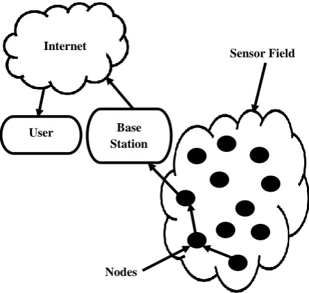
A wireless sensor network is a set of nodes arranged into a co-operative network. The concept of wireless sensor networks is based on digital electronics, micro-electro-mechanical systems (MEMS) and wireless communication technology [1]. In WSN nodes are arranged in form of clusters and networks that perform an assigned monitoring task without any human interference and resolutions [2]. Sensor nodes are able to sense physical environmental information, process the acquired data both at unit and cluster level and send the result to the cluster and one or more collection points named as sinks or base stations (as shown in Figure 1). However, node deployment is a major issue which is to be solved because a proper node deployment scheme reduces the delay and cost of the network with the increase in coverage, degree and lifetime of the network [3-4]. Wireless sensor network have found military applications in equipment monitoring, battlefield surveillance, reconnaissance and detection of nuclear, chemical, biological attacks [5]. They have also found wide civilian applications in environmental monitoring, disaster warning, medicine and home automation. The idea of deploying wireless sensor networks in the ocean to sense, survey and monitor phenomenon of interest is attractive to
[image:1.595.315.541.270.484.2]navies, maritime operators, environment monitoring agencies, offshore industry and scientific researchers [1-5].
Figure 1. Wireless Sensor Network Architecture
In wireless sensor networks, various types of node deployment schemes are used. All schemes are analyzed on the basis of performance parameters. These parameters are coverage, degree, delay and energy consumption. Above all network cost is also an important factor.
This paper has 7 sections. In Section 1 basic introduction of WSN has been discussed. In section 2 various node deployment models are discussed in detail. Section 3 highlights the various performance evaluation parameters. Section 4 highlights the existing schemes. In section 5 proposed scheme is discussed. Section 6 deals with the analysis of proposed scheme. Overall finding and opinion is concluded in section 7.
2.
NODE DEPLOYMENT MODELS
Node deployment models are broadly classified into two main categories i.e. random and deterministic node deployment .
User Base
Station Internet
Sensor Field
2.1
Random Node Deployment
In random node deployment, if there are “n” sensors, then they all have equal probability of being located, at any point inside a sensor field, which is shown in Figure 2. [6]
[image:2.595.76.280.125.266.2]
Figure 2. Random Node Deployment
In random node deployment nodes are scattered on those locations which are uncertain. Random node deployment can be done just by throwing sensor nodes from air. As a result of this there is tremendous change in node density because some nodes are placed closer to each other and some are placed away from each other. Random node deployment model is preferred where the deployment area is inaccessible such as volcanoes, seismic zones, etc. A random node deployment strategy can be cost effective only if it provides a desired coverage i.e. uses minimum sensor nodes to cover an area. But generally, it doesn’t works properly because the probability of throwing nodes on their exact locations is very less therefore an alternate approach is required.
2.2
Deterministic Node Deployment
In deterministic node deployment (as shown in Figure 3) the positions of nodes are predefined i.e. positions of the sensors are calculated before deployment and then the sensors are placed on their respective positions. The deterministic deployment is used in those missions where the deployment area is physically reachable. As compared to random deployment, deterministic deployment uses fewer number of sensor nodes to cover a given area. Therefore it is more preferable over random deployment. [6]
[image:2.595.316.537.293.490.2]
Figure 3. Deterministic Node Deployment
3.
PERFORMANCE PARAMETERS
In WSN, there are various performance parameters which have been considered for a node deployment scheme.
3.1
Coverage
Coverage is an important issue in WSN and it is related with energy saving, connectivity and network reconfiguration. In WSN applications, full coverage and a partial coverage both are measured. Here full coverage means that every point in the sensor field must be covered by at least one sensor without leaving any uncovered area. In some cases for e.g. temperature and pressure sensing environment, partial coverage can be consider which is similar to full coverage because in such cases reading at one point is similar to the surrounding area. K-coverage is the method of defining conditions on coverage. Here k-coverage represents the minimum coverage [6-7]. A network is said to have k-coverage if every point in it is covered by at least k sensors. And for this k-coverage map is used, which checks all possible coverage areas and the relative frequency of exactly k-covered points. An example of k-coverage map is shown in Figure 4, here 3 represents that area which is covered by 3 sensors where as 2 represents that area which is covered by 2 sensors.
Figure 4. An example of k-coverage map
3.2
Degree
It is also termed as connectivity of the network. The degree of the node defines the number of nodes lies in the transmission range “asense” of that particular node [6-7]. The higher the
degree, the more difficult it is to disconnect the node. But generally wireless sensor nodes are operated in unsafe environment. Many times the network connectivity fails due to displacement, communication breakage and frequent failure of nodes. The disconnected sub-networks are unable to communicate with the sink and cannot be able to send its data to base station. Therefore degree plays an important role in the successful deployment of WSN.
3.3
Energy Consumption
Energy is the most critical issue in WSN therefore it is necessary to optimize energy consumption in various ways. The layered architecture of typical wireless sensor node is projected in Figure 5, which consists of a sensing subsystem including one or more sensors with associated analog to digital converters (ADC) for data acquisition, a processing subsystem including a micro-controller unit (MCU) and memory for local data processing, a radio subsystem for wireless data communication and a power supply unit [8]. Nodes
Sensor Field
Sensor Field
Nodes
3 3
3 3
2
2 2
2
[image:2.595.71.276.544.700.2]International Journal of Computer Applications (0975 – 8887) Volume 88 – No.9, February 2014
Figure 5. Layered Architecture of a Wireless Sensor Node
Depending on the specific application, sensor nodes may also include some additional components such as a location finding system to determine their position, a mobilizer to change their location or configuration. Wireless sensor network consumes energy during sensing, processing and transmitting stage, and to reduce the overall energy consumption of the network and to make the system life-long different power management techniques are employed on different levels of the network. If direct communication is used in WSN from a source node to a sink node, then this will be very expensive in terms of energy. For this reason multi-hop communication must be consider in WSN to reduce the overall energy consumption [9]. A proper node deployment scheme is mandatory which reduces the energy consumption and extends the lifetime of WSN.
3.4
Delay
Delay is also an important constraint in WSN. Node deployment scheme affects the network delay in many aspects. If the distance between two nodes is more, than the time delay automatically get increased. On the other hand if distance is less than time delay is also getting reduced. Delay and energy are also related with each other, if delay is more than energy consumption also increases and vice-versa. Therefore a proper node deployment scheme ultimately resolves all above conflicts [10].
3.5
Cost Effectiveness
Network cost is another factor whose effect cannot be denied in the successful implementation of WSN. The node deployment scheme must be cost effective which fulfil all the goals i.e. providing a better coverage with fewer nodes, increases the degree and lifetime of the network with the reduction in delay [6-7].
4.
EXISTING SCHEMES
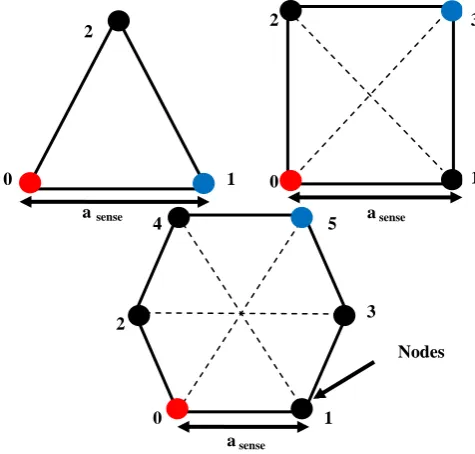
[image:3.595.53.288.68.243.2]Here three competitors of deterministic node deployment scheme for a sensor network i.e. a triangle, a square and a hexagon grid schemes are analyzed on the basis of number of required nodes, coverage, degree, delay and energy consumption [10]. Based upon detailed study and analysis a new approach is proposed which gives better results from these three existing schemes. The three existing schemes are shown in Figure 6.
Figure 6. Existing Schemes of Node Deployment
In case of triangle grid deployment the total area is divided into small triangles and nodes are placed on the edges of the triangle. All sides of the triangle are of equal size represented by “a sense”. In case of square grid deployment total area is
divided into small squares and nodes are placed at the corners of the square. The side of the square is also “a sense”. In
hexagon scheme nodes are placed on the six edges of the hexagon and here “a sense” again represents the side of the
hexagon.
5.
PROPOSED SCHEME
There are many ways in which sensor nodes can be deployed in the sensing field. Here a new and efficient approach for node deployment is being discussed in which nodes are deployed in a special manner which reduces the total number of nodes to be deployed, increases the coverage, degree of the network , reduces the delay and above all energy efficient. Here a circular shape is considered in which nodes are placed at the center and at the ends of the diameter. (as shown in Figure 7)
Figure 7. Proposed Scheme Power Supply Unit
Mobilizer with Location Finder
Radio
Processing Subsystem
Sensing Subsystem
Buffer MCU ADC Sensors
asense a sense
a sense
Nodes
a sense
0 1
2
0 1
2 3
0 1
2 3
4 5
0 1 2
3
[image:3.595.330.557.544.707.2]schemes with the proposed scheme on the basis number of required nodes, coverage, degree, delay and energy consumption is discussed.
6.1
Number of Required Nodes
To find out the number of required nodes (Nnodes) in a
specified area (A total area), it should be divided by the average
[image:4.595.315.552.102.277.2] [image:4.595.52.282.222.409.2]number of required nodes [6-7]. For various schemes total number of nodes can be calculated by using formulae listed in Table 1.
Table 1. Formulae used to calculate number of required nodes for various schemes
Schemes Number of Required Nodes
Triangle
Square
Hexagon
Proposed
[image:4.595.314.551.448.744.2]For the proposed scheme “L” represents the length and “B” represents the breadth of the sensor field. By using above formulae, it has been concluded that proposed scheme uses less number of nodes as compared to other three schemes. Here the number of required nodes for different schemes is calculated for 108 m2 area with sensing ranges of 10, 20 and 30 meters. The results are presented in Table 2.
Table 2. Number of nodes in 108 m2 area with sensing radius of 10, 20 & 30 meters in different schemes
Area(m2)
Scheme
108
a sense = 10m
108
a sense = 20m
108
a sense = 30m
Triangle 1150000 287500 127777
Square 1000000 250000 111111
Hexagon 777777 192500 85555
Proposed 751000 188000 83834
From Table 2 it is clear that as sensing range i.e. a sense
increases proposed scheme uses fewer nodes as compared to existing schemes. From Table 2 it is clear that to cover 108 meter square area, triangle scheme uses maximum number of nodes whereas proposed scheme uses minimum number of
Figure 8. Number of nodes used in 108 meter square area in various schemes when radius asense is 10, 20, 30 meters
6.2
Coverage and Degree
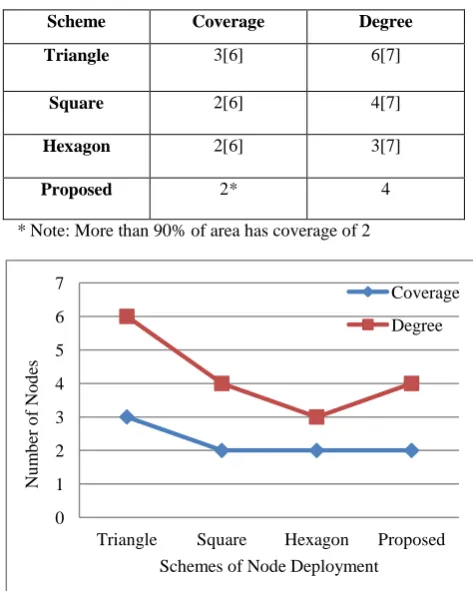
Coverage and degree of different deployments is affected by their sensing and communication radius. The proposed scheme has two-coverage and a degree of four. Two-coverage means that every point of the specified area is covered by at least two sensor nodes and a degree of four means that it covers four nodes within its transmission range. Table 3 shows that proposed scheme provides better coverage and degree than other deployments. Figure 9 shows the graphical results for Table 3.
Table 3. Coverage and Degree related to different schemes
Scheme Coverage Degree
Triangle 3[6] 6[7]
Square 2[6] 4[7]
Hexagon 2[6] 3[7]
Proposed 2* 4
* Note: More than 90% of area has coverage of 2
Figure 9. Coverage and Degree of various schemes 0
200000 400000 600000 800000 1000000 1200000 1400000
10 m 20 m 30 m
Sensing Radius asense
Triangle Square Hexagon Proposed
Nu
m
b
er
o
f
No
d
es in
1
0
8 m 2 A
re
a
0 1 2 3 4 5 6 7
Triangle Square Hexagon Proposed Schemes of Node Deployment
Coverage Degree
Nu
m
b
er
o
f
No
d
es
N nodes = 1.15 A total area / a sense 2
N nodes = A total area / a sense 2
N nodes = 0.77 A total area / a sense2
N nodes = (L / 2a sense) (B / a sense + 1)
[image:4.595.50.282.536.693.2]International Journal of Computer Applications (0975 – 8887) Volume 88 – No.9, February 2014
The graphical results shown in Figure 8 and 9 conclude that proposed scheme uses fewer nodes as compared to the existing schemes. In addition to this coverage of proposed scheme is similar to the square and hexagon scheme but have degree greater than the hexagon scheme.
6.3
Delay and Energy Consumption
To calculate delay NS2 software is used, here it is considered that the distance between two nodes is fixed and it is of 100 meters. In case of triangle grid deployment (as shown in Figure 6) if node 0 is the source node and node 1 is the sink node then there are two possible paths for packet transmission, one is the direct path i.e. from 0-1 and other is from 0-2-1. In case of square grid deployment if node 0 is the source node and node 3 is the sink node then there are three possible paths for packet transmission.One is the direct path i.e. from 0-3 and other paths may be 0-2-3 or 0-1-3. Delay measurement for triangle and square grid are shown in Table 4 and 5.
Table 4. Delay Measurement related to Triangle Grid Deployment
Delay Measurement in Triangle Grid Deployment ( in seconds)
Paths For Packet Transmission
Node 0 to 1 90 x 10-3
[image:5.595.317.552.173.465.2]Node 0 to 2 to 1 180 x 10-3
Table 5. Delay Measurement related to Square Grid Deployment
Delay Measurement in Square Grid Deployment ( in seconds)
Paths For Packet Transmission
Node 0 to 3 95 x 10-3 Node 0 to 2 to 3 180 x 10-3
Node 0 to 1 to 3 180 x 10-3
[image:5.595.51.284.307.522.2]In case of hexagon grid deployment if node 0 is the source node and node 5 is the sink node then there are five possible paths for packet transmission. One is the direct path i.e. from 0-5. Other paths may be 0-2-5 or 0-2-4-5. Similarly 0-1-5 or 0-1-3-5, Delay measurements for hexagon scheme are shown in Table 6.
Table 6. Delay Measurement related to Hexagon Grid Deployment
Delay Measurement in Hexagon Grid Deployment ( in seconds)
Paths For Packet Transmission
Node 0 to 5 260 x 10-3 Node 0 to 2 to 5 270 x 10-3
Node 0 to 2 to 4 to 5 270 x 10-3 Node 0 to 1 to 5 270 x 10-3 Node 0 to 1 to 3 to 5 270 x 10-3
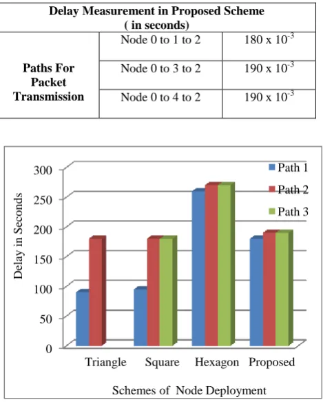
In proposed scheme (as shown in Figure 7) if node 0 is the source node and node 2 is the sink node then there are three possible paths for packet transmission.One path is from 0-1-2. Other paths may be 0-3-2 or 0-4-2. In all cases red node represents the source node and blue node represents the sink node. Delay measurements for proposed scheme are shown in Table 7.
Table 7. Delay Measurement related to Proposed Scheme
Delay Measurement in Proposed Scheme ( in seconds)
Paths For Packet Transmission
Node 0 to 1 to 2 180 x 10-3 Node 0 to 3 to 2 190 x 10-3 Node 0 to 4 to 2 190 x 10-3
Figure 10. Delay Measurement in various schemes
As evident from figure 10 it is clear that in case of hexagon scheme, all the three paths provide larger delay as compared to the proposed scheme. In addition to this in hexagon scheme the source node 0 consumes more energy for packet transmission because the distance between source 0 and sink 5 is larger as compared to proposed scheme. Therefore proposed scheme is a better alternative over hexagon scheme.
7.
CONCLUSION
In this paper, the two major deployment models are summarized along with a new modified approach. In WSN coverage and degree are important performance parameters, but taking parameters such as energy consumption, delay and cost effectiveness can make the node deployment more robust. The proposed scheme resolves the problem of using large number of sensor nodes. Therefore it is cost effective as compared to the existing schemes. Proposed scheme has a coverage of two which is similar to the square and hexagon scheme but the average percentage area covered by the proposed scheme has coverage of three. The degree of proposed scheme is similar to square scheme i.e. four but greater than the hexagon scheme i.e. three. Proposed scheme provides smaller delay over hexagon scheme and consumes less energy. Proposed scheme is energy efficient and is better in many aspects from other available schemes.
0 50 100 150 200 250
300 Path 1
Path 2 Path 3
De
lay
in
S
ec
o
n
d
s
Triangle Square Hexagon Proposed
[image:5.595.49.287.633.765.2]8.
REFERENCES
[1] I.F.Akyildiz, W. Su, Y. Sankarasubramaniam E. Capirci 2002, “Wireless Sensor Networks: a Survey”, Computer Networks, Vol 38, N. 4.
[2] C. Alippi, G. Anastasi, M. Di Francesco and M. Roveri 2009,“Energy management in Wireless Sensor Networks with energy-hungry sensors”, in IEEE Instrum. and Meas. Magazine, Vol. 12, No. 2, pp. 16–23.
[3] S. Faye and J. F. Myoupo 2011, “An ultra hierarchical clustering based secure aggregation protocol for wireless sensor networks,”Advances in Information Sciences and Service Sciences, vol. 3, no. 9, pp. 309–319.
[4] A. Abbasi and M. Younis 2007, “A survey on clustering algorithms for wireless sensor networks,” Computer Communications, vol. 30, pp.2826-2841.
[5] I. F. Akyildiz, T. Melodia, K.R. Chowdhury2007, “A Survey on Wireless Multimedia Sensor Networks”, Computer Networks, Vol. 51, Issue 4, pp. 921-960. [6] W. Y. Poe, J. B. Schmitt 2009, ‘‘Node deployment in
large wireless sensor networks: coverage, energy
consumption, and worst-case delay”, Proceedings of Asian Internet Engineering Conference, pp. 77-84. [7] E .S. Biagioni, G .Sasaki 2002, ‘‘Wireless sensor
placement for reliable and efficient data collection”, Proceedings of the 36th Annual Hawaii International Conference on System Sciences 0-7695-1874-5.
[8] R. Jurdak, A. G. Ruzzelli and G. M. P. O Hare 2010, “Radio Sleep Mode Optimization in Wireless Sensor Networks”, in IEEE Trans. on Mobile Computing, Vol. 9, No. 7, pp. 955–968.
[9] G. Anastasi, M. Conti, M. Di Francesco 2009, A. Passarella, “How to Prolong the Lifetime of Wireless Sensor Networks”, Chapter 6 in Mobile Ad Hoc and Pervasive Communications, (M. Denko and L. Yang, Editors), American Scientific Publishers, Vol. 12, N. 2, pp. 16-23.