DegNorm: normalization of generalized transcript degradation improves accuracy in RNA seq analysis

M E T H O D

Open Access

DegNorm: normalization of generalized

transcript degradation improves accuracy

in RNA-seq analysis

Bin Xiong, Yiben Yang, Frank R. Fineis and Ji-Ping Wang

Abstract

RNA degradation affects RNA-seq quality when profiling transcriptional activities in cells. Here, we show that transcript degradation is both gene- and sample-specific and is a common and significant factor that may bias the results in RNA-seq analysis. Most existing global normalization approaches are ineffective to correct for degradation bias. We propose a novel pipeline named DegNorm to adjust the read counts for transcript degradation heterogeneity on a gene-by-gene basis while simultaneously controlling for the sequencing depth. The robust and effective performance of this method is demonstrated in an extensive set of simulated and real RNA-seq data.

Keywords:RNA-seq, Normalization, RNA degradation, Degradation normalization, Alternative splicing, Non-negative matrix factorization

Background

RNA-seq is currently the most prevailing method for profiling transcriptional activities using high-throughput sequencing technology [1]. The sequencing tag count per unit of transcript length is used to measure the rela-tive abundance of the transcript [2]. Various factors exist that may affect the faithful representation of transcript abundance by RNA-seq read counts. Normalization is a crucial step in post-experiment data processing to en-sure a fair comparison of gene expression in RNA-seq analysis [3, 4]. The most commonly used approach is to normalize the read counts globally by a sample-specific scale factor to adjust the sequencing depth. Choices of the scale factor include the total number of reads (or mean), median, trimmed mean of M values [5], and upper quartile [3]. The second type of normalization aims to remove the read count bias due to physical or chemical features of RNA sequences or uncontrollable technical aspects. The GC content is known to affect the read counts in a nonlinear way [6,7], and this effect can be sample specific under different culture or library preparation protocols [8]. Systematic bias may also arise due to technical effects such as library preparation and sequencing batches. Such systematic biases can be

quantified and removed using factor analysis provided that the unwanted variation is uncorrelated with the covariates of interest [9,10].

Another type of bias arises from cDNA fragmentation and mRNA degradation. The RNA-seq assay requires fragmenting the cDNA (reversely transcribed from mRNA) or mRNA for high-throughput sequencing. Ideally, for a complete, non-degraded transcript, if the fragmentation is completely random, we expect to see reads uniformly distributed along the transcript. Never-theless, the fragmentation by random priming is not truly random due to primer specificity [11–13]. Conse-quently, read count per unit length of a transcript may not strictly reflect the transcript abundance when com-paring the expression of different genes. For the same gene, assuming the same protocol is applied to different samples, the bias attributable to fragmentation across samples should be similar. Thus, fragmentation bias is less problematic in a gene-by-gene differential expres-sion (DE) analysis. In contrast, mRNA degradation can vary substantially in both extent and pattern between genes and between samples [14,15]. The mRNA degrad-ation has different pathways and can happen in any re-gion of a transcript [16]. Perfect control of sample degradation during the experiment is difficult, particu-larly when the samples are collected from field studies

© The Author(s). 2019Open AccessThis article is distributed under the terms of the Creative Commons Attribution 4.0 International License (http://creativecommons.org/licenses/by/4.0/), which permits unrestricted use, distribution, and reproduction in any medium, provided you give appropriate credit to the original author(s) and the source, provide a link to the Creative Commons license, and indicate if changes were made. The Creative Commons Public Domain Dedication waiver (http://creativecommons.org/publicdomain/zero/1.0/) applies to the data made available in this article, unless otherwise stated. * Correspondence:[email protected]

or clinical samples. More importantly, different genes may degrade at different rates [17], which makes it im-possible to remove this bias by normalizing the read counts of all genes in the same sample by the same constant.

While the major impact of RNA degradation on gene expression analysis has been well recognized [17, 18], methods for correcting the degradation bias have not been fully explored in the literature. A few methods have been proposed to quantify the RNA integrity including RNA integrity numbers (RIN) [19], mRIN [20], and tran-script integrity number (TIN) [13]. The RIN gives a sample-specific overall RNA quality measure, but not at the gene level. In practice, a sample with RIN≥7 (on a scale of 0 to 10) is often regarded as having good quality. The mRIN and TIN measures were both defined in the gene level by comparing the sample read distribution with reference to the hypothetical uniform distribu-tion. In real data, due to GC content bias, primer specificity, and other complexities, the read count may substantially deviate from the uniform distribu-tion along the transcript [7].

To reduce the degradation effect, Finotello et al. pro-posed to quantify the exon-level expression by the max-imum of its per-base counts instead of the raw read counts [21]. If a given exon is in a more degraded re-gion, the local maximum may still be an underestimate of true abundance. On the other hand, the larger vari-ance associated with the local maximum (e.g., spikes) may result in instability in DE analysis. Based on the TIN measure, Wang et al. proposed a degradation normalization method based on loess regression of read counts on the TIN measure for genes within the same sample [13]. However, the uniform baseline assumption and the failure to compare gene-specific degradation across samples appear to be the two major limitations, which may lead to extreme variability and bias in DE analysis (to be shown below). Jaffe et al. proposed a quality surrogate variable analysis (qSVA) to remove the confounding effect of RNA quality in DE analysis [22]. They investigated the degradation of RNA-seq data from dorsolateral prefrontal cortex (DLPFC) tissue under two different RNA-seq protocols, namely, poly(A)+ (mRNA--seq) vs. ribosomal depletion (Ribo-Zero-(mRNA--seq). Thousands of features significantly associated with degradation were identified under either protocol separately, while no overlap was found between the two protocols. Further-more, comparing the DLPFC samples and the peripheral blood mononuclear cell (PBMC) samples [17] both se-quenced under the same poly(A)+ protocol, they found only four shared features. It is unclear how the sequence features identified in this study can be generalized for degradation bias correction in other RNA-seq data in practice.

Alternative splicing is frequently observed in higher organisms, and it further complicates the gene expres-sion estimation in RNA-seq [23]. In the gene-level DE analysis, we test the equivalence of relative abundance of transcripts in copy numbers between samples or condi-tions. If the two samples have differential exon usage, read counts need to be adjusted accordingly to better represent the transcript relative abundance in the re-spective samples. Currently, most existing statistical packages for RNA-seq analysis (e.g., DESeq [24] and edgeR [25]) all take the raw read counts as input, while such complexities are completely ignored in practice.

In this paper, we propose a novel data-driven method to quantify the transcript degradation in a generalized sense for each gene within each sample. Using the estimated degradation index scores, we build a normalization pipeline named DegNorm to correct for degradation bias on a gene-by-gene basis while simul-taneously controlling the sequencing depth. The per-formance of the proposed pipeline is investigated using simulated data, and an extensive set of real data that came from both cell line and clinical samples sequenced in poly(A)+ or Ribo-Zero protocol.

Results

Data sets

We consider six RNA-seq data sets that were generated from cell lines or clinical samples under either the main-stream poly(A) enrichment (mRNA-seq) or ribosomal RNA depletion protocol (Ribo-Zero-seq). The first one was from a brain glioblastoma (GBM) cell line study of a human for the impact of RNA degradation on gene expression ana-lysis [26]. Technical replicates of RNA samples were frag-mented under different incubation time and temperature using the NEBNext Magnesium RNA fragmentation mod-ule. We chose to analyze nine mRNA-seq samples in three groups of three, corresponding to three average RNA integ-rity number (RIN) = 10, 6, and 4, respectively (to be re-ferred to as R10, R6, and R4 for simplicity). We will perform DE analysis for R10 vs. R4 and R6 vs. R4.

The second set contained 32 single-end mRNA-seq samples from human peripheral blood mononuclear cells (PBMC) of 4 different subjects: S00, S01, S02, and S03 [17]. The extracted RNA sample from each subject was kept in room temperature for 0, 12, 24, 36, 48, 60, 72, and 84 h, respectively, to approximate the natural degradation process. We choose S01 as an illustrating example and will perform DE analysis for 0 + 12 h vs. 24 + 48 h (results for other subjects are similar).

library with two runs for eight lanes each. We will run DE analysis of the first run vs. the second run. The second subset contained two biological conditions: condition A of five samples from the same Stratagene’s UHR RNA, and condition B of five samples from Ambion’s human brain reference RNA. The first four replicates from both condi-tions were prepared by the same technician while the fifth was by Illumina. We excluded the fifth sample from both conditions because they showed a dramatic difference in coverage curves compared to the rest.

The fourth data set contained RNA-seq data from dorso-lateral prefrontal cortex (DLPFC) tissue of five brains— three controls and two schizophrenia cases [22]. Each tissue was left in room temperature (off of ice) for 0, 15, 30, and 60 min for degradation. The RNA sample was extracted and prepared for both mRNA-seq and Ribo-Zero-seq. We chose to analyze one schizophrenia case (Br1729, results for other subjects are similar). We will perform DE analysis T0+T15 min vs. T30+T60 min under the same protocol, i.e., mRNA-seq or Ribo-Zero-seq, and then cross-platform DE analysis between the two protocols.

The fifth data set originated from three pairs of matched fresh-frozen (FF) and formalin-fixed paraffin-embedded (FFPE) tissues of three breast tumor patients (namely T1, T2, T3) with a moderate archival time of about 4–5 years [29]. The FFPE samples are typically partially degraded. We will analyze the mRNA-seq data of FF (500 ng) and FFPE (100 ng) to investigate whether the degradation normalization can help improve the DE analysis in fragmented clinical RNA samples.

The last data set arose from a clinical study on how AMP kinase (AMPK) promotes glioblastoma bioenergetics and tumor growth [30]. It was shown that cancer cells can acti-vate AMPK and highjack the stress-regulating pathway in cells. Thus, inhibiting AMPK in cancer cells may lead to treatment of GBM. RNA-seq data was collected from two patient-derived GBM stem cell (GSC) lines (GBM9 and GBM10) between control and AMPK knockout to identify differentially expressed genes. We will perform DE analysis between the three control and three knockout samples in GBM10 cell line. Unlike the first five sets where the ground truth of gene expression was known or mostly verified, the AMPK knockout data represents a typical case in clinical studies where only a handful genes of interest, most often suspected as differentially expressed, were PCR verified. For this reason, in the following analysis, we will compare the different normalization methods by benchmarking our ana-lyses using the first five sets and then present the AMPK data as a case study in the last.

Non-uniformity and heterogeneity in read distribution pattern

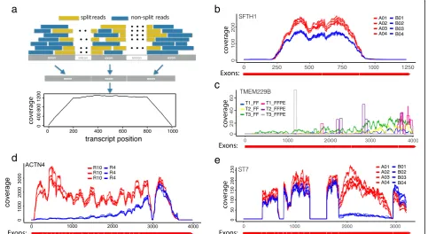
We define a total transcript as the concatenation of all annotated exons from the same gene. The read coverage

score at a given location within the transcript is defined as the total number of reads (single-end) or DNA fragments (paired-end) that cover this position (Additional file 1). If mRNA transcripts are complete and the fragmentation is random, we expect to see a flat coverage curve in the entire transcript except in the head and tail region (Fig. 1a). Nevertheless, in real data, the read coverage curves rarely display a uniform pattern; instead, dramatic and gene-specific differences are often observed across samples (Fig. 1b–e). The non-uniformity itself is less concerning as long as the coverage pattern is consistent across samples (Fig. 1b) such that the read counts can still faithfully represent the relative abundance of transcripts. In contrast, hetero-geneous coverage patterns are often observed where some samples show significantly decayed read counts in some regions (Fig.1c–e). One major cause of this hetero-geneity is mRNA degradation, which is clearly shown in the case of ACTN4 gene of R4 samples from the GBM data (Fig. 1d). Different sample preparation methods may lead to distinct read distributions. For example, FFPE samples may show a highly localized discrete read distribution pattern in contrast to a continuous distribu-tion typically observed in FF samples (Fig. 1c). Alterna-tive splicing may also result in depleted read count in the entire region of an exon, as exemplified in the ST7 gene of B samples (region 1900–2900 bp) from the SEQC-AB data (Fig.1e). For the gene-level DE analysis, loss of read count due to such complexities needs to be compensated to ensure unbiased quantification of gene expression.

Generalized degradation and degradation normalization algorithm

The degradation we target to normalize is defined in a generalized sense. Any systematic decay of read count in any region of a transcript in one or more samples com-pared to the rest in the same study is regarded as deg-radation. Clearly, mRNA degradation is one main cause, but alternative splicing and other factors may be the confounders that are difficult to deconvolute. To avoid confusion, in the following context, we will reserve the term “mRNA degradation” for the physical degradation of mRNA sequences, and “degradation” or “transcript degradation” for the generalized degradation without specification.

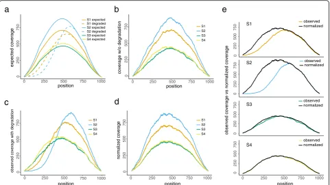
the expected coverage curve for the given gene within each sample if no degradation occurs. Degradation may occur in any region of the transcript to cause negative bias in the observed read counts. To illustrate this, we generated four expected coverage curves of identical shape but with different abundance levels (Fig. 2a), among which samples S1 and S2 are subject to degrad-ation in the 5′end with different patterns. Based on the expected curves, we further simulated a random realization of four complete curves with sampling error imposed (Fig. 2b, to be referred to as latent curves) and two degraded for sample S1 and S2, respectively (Fig.2c). The NMF-OA algorithm takes the four observed cover-age curves (i.e., two non-degraded (S3 and S4) and two degraded (S1 and S2)) as input and estimates the latent curves by minimizing the squared distance between the observed and latent, subject to the constraint that the la-tent curves must dominate their respective observed curves at all positions (Figs. 2d, e; the “Methods” sec-tion). We define the degradation index (DI) score for each gene within each sample, as the fraction of area

covered by the estimated latent curve, but above the ob-served curve (Fig. 2e). It measures the proportion of missing read count due to degradation given the current sequencing depth.

The DegNorm pipeline iteratively corrects for degrad-ation bias while simultaneously normalizing sequencing depth. First, the NMF-OA algorithm is applied to se-quencing depth-normalized read counts for all genes one by one to estimate the DI scores. Second, the result-ing DI scores are then used to adjust the read counts by extrapolation for each gene. The adjusted read counts are used to normalize the raw data for sequencing depth. These two steps are repeated until the algorithm con-verges (the“Methods”section).

DI score as sample quality diagnostics

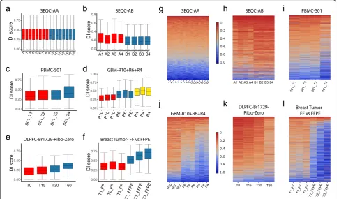
The estimated DI scores provide an overview of the within-sample, between-sample, and between-condition variation of degradation extent and patterns. We plotted the DI scores in three ways: a box plot of DI scores for each sample (Fig. 3a–f ), a heatmap of the DI scores

a

b

d

c

e

sorted in ascending order of the average scores of the first condition defined in the DE analysis (Fig.3g–l), and a pairwise correlation matrix of DI scores between sam-ples (Additional file2: Figure S1a-f ).

For SEQC-AA data with 16 technical replicates, the median of DI scores is ~ 0.35, consistent across samples (Fig. 3a). While the degradation pattern varies between genes, no systematic between-condition difference is ob-served (Fig.3g, Additional file2: Figure S1a). In contrast, for the SEQC-AB data, the 4 samples from condition B have relatively lower and more homogeneous degrad-ation than that from A samples (Fig. 3b). Many genes show a condition-specific clustered pattern in DI scores (Fig.3h), resulting in a high within-condition correlation (Additional file2: Figure S1b).

The PBMC and GBM data are known to have differen-tial mRNA degradation. The DI scores of PBMC S01 data confirm a progressive deterioration of average deg-radation when samples underwent degdeg-radation in room temperature for 0, 12, 24, and 48 h, respectively (Fig.3c, i, Additional file2: Figure S1c). The degradation from 24 to 48 h was particularly accelerated compared to the first 24 h. The nine GBM samples were previously classified into three groups according to the RNA integrity

number (RIN), R= 10, 6, and 4, respectively. The DI scores show a clear escalating pattern of degradation se-verity across the three groups (Fig.3d, j) with two strong clusters, i.e., R10 vs. R6+R4 (Additional file 2: Figure S1d). The scatter plots of DI scores further exemplify a higher correlation between samples within the same RIN group than across different RIN groups (Additional file2: Figure S1 g-i).

For the DLPFC Br1729 Ribo-Zero-seq data, DegNorm recovered an increasing pattern of degradation from time 0 to 60 min as expected (Fig.3e, k, Additional file2: Figure S1e). The three pairs of breast tumor samples were prepared in two different ways—fresh frozen (FF) and formalin-fixed paraffin-embedded (FFPE)—but both sequenced under the mRNA-seq protocol. The DI scores confirm that the mRNA transcripts in FFPE samples tend to be highly degraded compared to the paired FF samples (Fig. 3f, l), and degradation pat-terns are strongly clustered within the same FF or FFPE group (Additional file 2: Figure S1f ).

In summary, the DI scores from the DegNorm provide meaningful quantification of gene-level degradation be-tween samples for both cell line and clinical samples under both mRNA-seq and Ribo-Zero-seq protocols.

0 250 500 750 observed co v er

age with degradation

0 250 500

position 750 1000 0 250 500 750 normalized co ver age

0 250 500 750 1000

position S1 S2 S3 S4 S1 S2 S3 S4 0 250 500 750

0 250 500 750 1000

0 250 500 750 0 250 500 750 0 250 500 750 position observed co v er

age vs normalized coverage

a

b

c

d

e

0 250 500 750 1000

0 250 500 750 expected co v er age position 0 250 500 750

0 250 500 750 1000

co

v

erage w/o degradation

position S1 S2 S3 S4 normalized observed observed normalized observed normalized S1 expected S1 degraded S2 expected S2 degraded S3 expected S4 expected

The degradation pattern is gene-specific, and the deg-radation extent may vary substantially between samples or conditions.

DegNorm improves accuracy in gene expression analysis

We set out to evaluate how the proposed DegNorm pipeline may improve differential expression analysis by comparing it with other seven normalization methods including UQ [3], TIN [13], RUVr, RUVg [10], trimmed mean of M values (TMM) [5], relative log expression (RLE) [24], and total read count (TC) [4]. The RUV methods were designed to remove unwanted variation, but it is unclear whether it is effective for correcting degradation bias. We dropped the RUVg method from the main text for its performance can be very sensitive to the choice of empirical control genes (Additional file2: Figure S2a-f ) or the choice of factor(s) from the factor analysis in the estimation of unwanted variation (Additional file 2: Figure S2 g, h). The TMM, RLE, TC,

and UQ methods yielded very similar results in all data we analyzed in this paper (Additional file2: Figure S3a-f for some examples). For visualization purpose, only the UQ results are presented in the main figures.

We first examine the five data sets that originated from the samples that had no true biological difference between conditions under test (i.e., SEQC-AA, PBMC-S01, GBM, DLPFC, and breast tumor). RNA deg-radation induces bias and thus may cause extra variance. Severe degradation may even result in a difference of transcript abundance for some genes when they are pre-pared for RNA-seq. Thus, we investigate how different methods may reduce variance by plotting the coefficient of variation (CV) of normalized read count vs. mean read count in log scale (the logged mean was linearly transformed to 0–1 range, Fig. 4a–f ). Overall, the TIN method gives a relatively larger CV than the other three methods. When RNA degradation is a major concern such as in GBM-R10vsR4, and breast tumor FF vs. FFPE comparisons, DegNorm pronouncedly reduced the CV

a

b

g

h

i

c

d

e

f

j

k

l

Fig. 3Degradation index (DI) scores show gene-/sample-/condition-specific degradation heterogeneity.a–fBox plots of DI scores presented in a between-group comparison defined for the differential expression analysis as follows.aSEQC-AA data (16,670 genes): the 8 (1–8) technical replicates from the first run vs. the 8 (9–16) from the second run.bSEQC-AB data (19,061 genes): 4 biological replicates from A condition vs. 4 from B condition.

compared to other methods except in the very lower or upper end where the CV was inflated due to outliers

(Fig. 4d, f ). The RUVr approach applies UQ

normalization first and then further removes the add-itional variation estimated from the factor analysis. It always reduces CV over the UQ method.

We normalized the raw read count by dividing it by 1 - DI score for each gene within each sample. The ad-justed read counts (rounded) were input into the edgeR package [25] for DE analysis. When all genes are true nulls, the empirical cumulative distribution function (ECDF) ofpvalue tends to be a diagonal line. Thus, an ECDF curve closer to the diagonal line indicates better performance of the normalization method in correcting the degradation bias. For SEQC-AA data with 16 technical replicates, all 4 methods resulted in expected ECDF curves close to the diagonal line (Fig. 4g). For

PBMC-S01 and GBM-R6vsR4 comparisons with known modest between-condition difference in mRNA degrad-ation, the ECDF curves from different methods were all well above the diagonal line (except TIN for PBMC data), suggesting that differential degradation probably has caused a difference in gene abundance level when the samples were sequenced (Fig.4h, i). Both DegNorm and TIN methods brought the ECDF curve down to-wards the diagonal line compared to UQ and RUVr, in-dicating that correction for degradation bias helps reduce potential false positives. Nevertheless, the TIN curve in PBMC-S01 data was well below the diagonal line (Fig. 4h), which may indicate a loss of statistical power due to the large variance of the normalized read counts (Fig. 4b). In contrast, the RUVr ECDF curves in both comparisons are significantly higher than that in UQ (regardless that RUVr had lower CV than UQ),

a

b

g

h

c

d

i

j

e

f

k

l

suggesting an ineffective correction of degradation bias or even an adverse effect to cause extra false positives. For the GBM-R10vsR4 comparison, ECDF curves are all far above the diagonal line, likely indicating a substantial change of transcript abundance level for many genes due to drastic degradation in R4 samples (Fig.4j).

The DLPFC and breast tumor FF-FFPE RNA-seq data were both generated from clinical tissue samples. For the DLPFC Br1729 T0+T15 vs. T30+T60 com-parison, the DegNorm resulted in a slightly lower p value than UQ in Ribo-Zero (Fig. 4k) but much lower than UQ in mRNA-seq (Additional file 2: Figure S4a) data. For the breast tumor data, FFPE samples were shown substantially fragmented and degraded than FF samples (Figs. 1c and 3f). DegNorm resulted in a lower p value curve than all other methods (Fig. 4l). We also did cross-protocol DE analysis by comparing the four Br1729 mRNA-seq with four Ribo-Zero sam-ples. All p value curves were way above the diagonal line (Additional file 2: Figure S4b), suggesting DE analysis across different sequencing protocols should not be recommended.

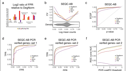
Thepvalue ECDF curve provides a global picture of a false-positive rate at different type-I error rate thresholds when all null hypotheses are true. In practice, as the ground truth is unknown, one typically claims the DE by controlling the false discovery rate (FDR) to correct mul-tiple comparison errors. Thus, we further compared the false-positive rate of different methods by controlling the nominal FDR under the criterion of q value ≤0.05 using q-value package [31–33]. For SEQC-AA data with a little degradation difference between samples, all four methods resulted in very few claimed positives (Additional file 3: Table S1), consistent with the close-to-diagonal-line nature ofp value ECDF curves in Fig.4g. For the rest data with differential degradation, all methods yielded a substantial number of false positives. For comparison, we plotted the ratio of the false-positive rate of UQ, RUVr, and TIN over DegNorm in log2 scale (Fig. 5a). The UQ and RUVr methods consistently yielded more false positives than DegNorm, by a factor ranging from 1 to 3.7 and 1.4–36.8, respectively. The TIN method reduced the false-positive rate over Deg-Norm in the PBMC-S01 with a factor of 1.37.

a

b

d

e

c

0.00 0.25 0.50 0.75 1.00 SEQC-AB p-value ECDF UQ DegNorm RUVr TIN 0.75 0.80 0.85 0.90

ROC curve AUC

1 2 3 4 5

PCR Log2FC threshold

0.95 UQ DegNorm RUVr TIN SEQC-AB PCR

verifed genes--set 1

0.00 0.25 0.50 0.75 1.00

0.00 0.25 0.50 0.75 1.00

TPR FPR UQ DegNorm RUVr TIN SEQC-AB PCR verifed genes--set 2

0.00 0.25 0.50 0.75 1.00 TPR

0.00 0.25 0.50 0.75 1.00

FPR UQ DegNorm RUVr TIN SEQC-AB 0.4 0.5 0.6 0.7 0.8 0.9 CV UQ DegNorm RUVr TIN

Log mean counts

0.00 0.25 0.50 0.75 1.00

Density 6 5 4 3 2 1 0 -1 -2 -3 -4 GBM R10vsR4 GBM R6vsR4 PBMC-S01 DLPFC-Br1729 Ribo-Zero DLPFC-Br1729 Poly(A)+ Breast tumor FFvsFFPE

UQ RUVr TIN Log2 ratio of FPR relative to DegNorm

f

verifed genes--set 2

Nevertheless, we will show below that this relatively lower false-positive rate from the TIN method is an indi-cation of undermined power due to the excessively inflated variance (Fig.4a–f ).

The SEQC-AB data presents an atypical example con-taining an unusually large number of differentially expressed genes [27,34]. DegNorm produced an overall lower CV than UQ, RUVr, and TIN methods (Fig. 5b). The DegNorm ECDF lies below those of UQ and RUVr methods while above TIN (Fig.5c). With the presence of truly differentially expressed genes, the lower ECDF can be interpreted as a tendency to result in fewer false posi-tives (good) or more false negaposi-tives (bad, less power) or a mix in the DE analysis. To investigate this, we utilized 2 sets of PCR-verified genes, 1 from the original MAQC study of 843 genes [34] and the other from SEQC study of 20,801 genes [27], as the ground truth to construct re-ceiver operating characteristic curves (ROC) (Fig. 5d, e). Similar to Rissio et al. [10], we defined a gene as a posi-tive if the absolute value of log2 fold change≥2, a nega-tive if ≤0.1, and undefined otherwise. For both sets, the ROC curves suggest that DegNorm achieved better true-positive rate (sensitivity) than UQ, RUVr, and TIN while controlling the false-positive rate (1-specificity). For example, at FPR = 0.05 (specificity = 0.95), the larger PCR set suggested a 78.1% true-positive rate for Deg-Norm in comparison with 73.7%, 67.3%, and 48.3% for UQ, RUVr, and TIN methods, respectively. When we varied the of log2 fold change threshold value from 1 to 5 to define the positives, the area under the ROC curve (AUC) from all methods (except TIN) increased as expected, while the AUC from DegNorm remained the largest and the gap between DegNorm and other methods enlarge (Fig. 5f ). As the true-negative set was fixed in this experiment, the true-positive rate drove the change of AUC as the threshold value in-creases. This suggests DegNorm improves the power to identify highly differentially expressed genes over other normalization methods while controlling the false-positive rate. Therefore, we conclude that the lower ECDF curve from DegNorm method (Fig. 5c) manifests a good tendency to reduce false-positive rate or increase specificity without sacrifice of statis-tical power or sensitivity.

The RUVr and TIN methods both showed pronoun-cedly lower power than DegNorm and UQ, but due to different reasons (Fig. 5d–f ). The RUVr method is guaranteed to reduce more variation based on the UQ-normalized data. Nevertheless, the removed vari-ation may contain true biological difference if it is con-founded with unwanted variation, which will result in more false negatives. On the other hand, the large vari-ance incurred by TIN method appears to severely under-mine the power in the DE analysis (Fig.5b).

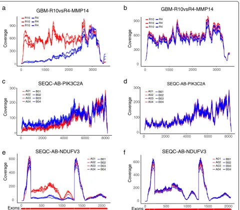
We present three examples that exemplify how DegNorm may improve the accuracy in the DE analysis. We used local false discovery rate (lfdr) from q-value package [31–33] to quantify the significance of DE ana-lysis. Compared toq value, which quantifies the average FDR for all genes with smaller p value than the given one, lfdr is more appropriate to quantify the false discov-ery rate associated with any individual p value. The MMP14 gene in the GBM-R10vsR4 comparison displayed a clear degradation in the 5′end in R4 samples (Fig.6a) and tested positive using UQ method (pvalue = 1.31e−8, lfdr = 1.1e−8). DegNorm compensated for the degraded portion of R4 samples and returned negative test result (p value = 0.91, lfdr = 0.32, Fig.6b). The second example is the PIK3C2A gene from SEQC-AB comparison, a PCR-verified negative with log2 fold change = 0.06. It tested positive under UQ (p value = 0.005, lfdr = 0.02) (Fig.6c) while negative under DegNorm with degradation correction in the 5′end of A samples (pvalue = 0.77, lfdr = 0.97, Fig. 6d). The third example is the NDUFV3 gene from the SEQC-AB data, showing nearly depleted cover-age in the entire third exon region from ~ 223 to 1327 nt for B samples likely due to alternative splicing. It tested positive under UQ (p value = 1.94e−37, lfdr = 3.39e−09, Fig. 6e). DegNorm returned a negative result (p value = 0.808, lfdr = 0.942, Fig. 6f ), consistent with negative PCR verification (log2 fold change =−0.114).

GBM AMPK knockout data

LDHA, SLC2A1, HK1, GPI, ALDOA, TPI1, PFKM, ENO1, GABPA, TFAM, and COX20, DegNorm, UQ, and RUVr all successfully identified 8 except HK1, PFKM, GABPA, and COX20, whereas TIN method missed 2 additional genes, GPI and ALDOA (Add-itional file 4: Table S2). The discrepancy between the RNA-seq set and PCR results could be due to cell line-specific variation, lack of power due to small sample size or sample quality (personal communication with Dr. Dasgupta). Clearly, such a small-scale verification is in-sufficient to conclude about the sensitivity, neither can we evaluate the specificity without verification of the negatives. The discrepancy between DegNorm and other

methods does provide alerts to users of possible false positives caused by degradation when interpreting the results of such studies.

Simulation study

To further systematically investigate the performance of DegNorm, we conducted a simulation study in a two-condition comparison: 4 control (A) vs. 4 treat-ment (B) samples in 4 different degradation settings. Each sample of 20,000 genes was simulated with a ran-dom sequencing depth of 40–60 million reads, 5% of which were chosen to be upregulated and another 5% for downregulated in expression. In the first setting, all

a

b

c

d

e

f

0 200 400 600

0 500 1000 1500 2000

Coverage

SEQC-AB-NDUFV3

Exons:

0 200 400 600

0 500 1000 1500 2000

Coverage

SEQC-AB-NDUFV3

Exons:

Coverage

SEQC-AB-PIK3C2A

A01 A02 A03 A04

B01 B02 B03 B04

Coverage

200

100

0

0 2000 4000

SEQC-AB-PIK3C2A

300

Coverage

600 900

0

0 1000 2000 3000

R10 R10 R10

R4 R4 R4

GBM-R10vsR4-MMP14

300

Coverage

600 900

0

0 1000 2000 3000

GBM-R10vsR4-MMP14

6000 8000 300

200

100

0

300

0 2000 4000 6000 8000

A01 A02 A03 A04

B01 B02 B03 B04

A01 A02 A03 A04

B01 B02 B03 B04

A01 A02 A03 A04

B01 B02 B03 B04 R10

R10 R10

R4 R4 R4

genes had no degradation whereas in the rest 3 settings, 80% of the genes were randomly selected for degrad-ation. In the second setting, for a gene selected for deg-radation, either 3, 4, or 5 samples out of the 8 were randomly chosen for degradation, whereas in the third, either all 4 control samples or 4 treatment samples were randomly chosen for degradation. In both second and third settings, the degradation extent for each de-graded gene was random but following the same distribu-tion. In the fourth setting, for each gene selected to degrade, 2 control samples were randomly selected for degradation with the same expected severity, while all treatment samples had a sample-specific systematic differ-ence in expected severity. The simulation details are de-scribed in the“Methods”section and Additional file1.

Simulation I presents a scenario where samples have no degradation bias or any other bias but only between-sample variation in sequencing depth. In the following, we shall refer the latent count as the true read count for a gene before degradation is imposed. Deg-Norm is data driven and always returns non-negative DI scores by design. The estimated DI scores have a median ~ 0.11 in all samples (Fig.8a), demonstrating the absence of between-condition heterogeneity (Fig.8b). To investi-gate how the positive bias in DI scores may impact DE analysis, we first plotted the normalized vs. latent read count from different methods (Fig.8c–f ) (the latent read count in simulation I is just the raw read count).

Unsurprisingly, the UQ method perfectly normalizes the sequencing depth (Fig.8c), while all other three methods caused bias or extra variance to different extents (Fig. 8d–f ). The positive bias from DegNorm is more pronounced when read counts are low such that read coverage curve cannot be well estimated (Fig.8e). As for any gene, all samples are subject to this over-estimation bias; this bias may partially cancel off in DE analysis. As a result, thepvalue ECDF and ROC curves of DegNorm almost perfectly overlap with the latent and UQ curves (Figs. 8g, h). At FPR = 0.05, DegNorm, RUVr, and TIN had sensitivity decay of 0.6%, 1.1%, and 8.6%, respect-ively, compared to using the latent counts or UQ method (Additional file5: Table S3).

When degradation is an issue as in simulations II–IV, the estimated DI scores provide an informative characterization of the overall degradation severity of each sample (Additional file 2: Figure S5a-f ) as well as the similarity of gene-specific degradation pattern be-tween samples (Additional file 2: Figure S5 g-l). DegNorm demonstrates consistently better correction of degradation bias than the UQ, TIN, and RUVr methods, as evidenced by higher regression coefficient of determination (R2), and a nearly symmetric distribution of data points around the diagonal line in the scatter plot of normalized vs. latent read counts (Fig. 9a–d, Additional file 2: Figure S6a-h). The UQ method does not correct for any degradation bias but instead only

a

b

d

e

c

normalizing sequencing depth (Fig.9a, Additional file2: Figure S6a, e). Similar extreme variance issue is also ob-served in the TIN method in simulations II–IV (Fig. 9b, Additional file 2: Figure S6b, f ).

To gain more insights into the CV plots, we singled out the 18,000 truly non-differentially expressed genes from simulations II–IV and plotted the CV against the mean of normalized count (Fig.9e–g). Without the con-founding effect of biological difference, the CV of these genes tends to be inflated due to degradation-caused loss of read count. Thus, the CV is an informative measure to assess the effectiveness of degradation normalization. Indeed, the UQ and RUVr curves are both well above the latent curve in all simulations, suggesting degrad-ation bias was not or inadequately corrected. Similar to what we observed in the real data, the TIN CV curve dominates other methods in each setting, echoing the excess of variance observed in the scatter plot (Fig. 9b, Additional file 2: Figure S6b, f ). In contrast, the DegNorm curves were the closest to the respective la-tent curves but with a slight underestimation of CV in the lower half.

DegNorm improves the accuracy in DE analyses. In both ECDF (Fig. 9h–j) and ROC plots (Fig. 8k–m), the DegNorm curve was the closest to the latent one, demon-strating improvement over other normalization methods

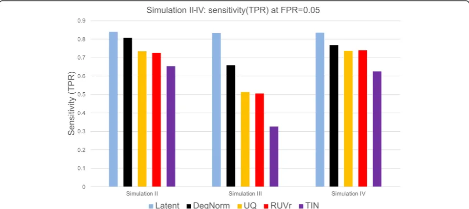
to different extents. We tabulated the sensitivity of each method at FPR = 0.05 (Additional file 5: Table S3) and plotted it in Fig. 10. In settings II and III, where degrad-ation was randomly chosen among samples (II) or condi-tions (III), the UQ and RUVr methods were both ineffective to correct this non-systematic but gene-specific bias (Figs.9k, land10). In particular, in simulation III as degradation was applied to one condition of random choice for a given gene, the degradation bias was com-pletely confounded with the covariate of interest and can-not be removed by UQ or RUVr method. Consequently, many false positives were called due to degradation bias (Fig.9l). At FPR = 0.05 threshold, DegNorm improved the sensitivity by a factor of 1.28, 1.30, and 2.01 compared to UQ, RUVr, and TIN methods, respectively (Fig. 10, Additional file 5: Table S3). In contrast, the treatment samples in setting IV had a systematic difference in aver-age degradation (Additional file 2: Figure S5c), both UQ and RUVr performed reasonably well (Figs. 9mand 10). In all four degradation settings, the TIN method showed inferior power to detect true DE genes.

Discussion and conclusions

In this paper, we showed that RNA degradation pattern and severity are not only sample specific, but also

gene-specific, and thus commonly used global

Fig. 8Results for simulation I.aBox plot of estimated DI scores where conditions A and B stand for control and treatment samples, respectively.

normalization methods that impose a sample-specific constant adjustment to all genes within the same sample are ineffective to correct for this bias. The RUVr ap-proach is guaranteed to reduce variation, while they failed to show pronounced improvement over the UQ method in the DE analysis in all data sets considered in this study (even got worse in all data under consider-ation). One complexity is that the true biological differ-ence is often confounded with degradation (e.g., SEQC-AB data) and other unwanted variation. The fac-tor analysis cannot well separate the unwanted from the wanted variation, and it may even remove the true biological difference of interest. This confounding issue was illustrated in the SEQC-AB data by the high within-condition and low between-condition correl-ation of DI scores (Additional file 2: Figure S1b). In particular, the RUVg method was sensitive to the selec-tion of empirical control genes or the factor(s) used to estimate the unwanted variation (Additional file 2: Figure S2a-j). More objective criteria in this regard need to be developed for the RUVg method.

Although motivated by mRNA degradation, we de-fined the degradation in this paper in a generalized and relative sense. The quantified DI scores may reflect con-founding effects from mRNA degradation, alternative splicing, and other factors. Risso et al. [10] showed that in the SEQC-AB data, samples were clustered due to the difference of sample preparation, experiment protocol, sequencing run batches and flow cell, etc. Such factors could impact the RNA samples by changing the read coverage curves. Thus, normalizing heterogeneity in coverage curves may help reduce bias due to such

factors. Indeed, in all five benchmark data sets consid-ered in this paper, DegNorm performed consistently bet-ter compared to other methods regardless of whether mRNA degradation was a known concerning issue. Un-like mRIN and TIN measures where degradation was de-fined as the deviation from hypothesized uniform coverage curve, the DI score from DegNorm is defined with reference to an adaptively estimated latent coverage curve that minimizes the distance to the observed cover-age curves. If a gene has 50% degradation but having consistent coverage curves across samples, the estimated DI scores will all be nearly 0. In this case, the read count in each sample can still accurately reflect the relative abundance between samples, and degradation correction is unnecessary. From this perspective, the DI score is de-fined in a relative sense. Normalizing the read counts for degradation bias using DI scores is hoped to minimize the extrapolation needed, thus avoids an excess of vari-ance. The advantage of this strategy was exemplified in all real and simulated data sets in contrast to the TIN method.

RNA samples are always desirable in RNA-seq. Further-more, cross-platform DE analysis is not recommendable. Second, the core component of DegNorm is a matrix factorization over-approximation algorithm aiming to correct for the degradation bias that commonly exists in RNA samples, even for the high-quality SEQC data.

DegNorm tends to result in a pronounced

over-estimation bias in DI scores for genes with low read counts regardless of whether degradation is present (simulations II–IV) or absent (simulation I). We showed in simulation I that this bias is not a big concern in DE analysis as it tends to be homogeneous across all sam-ples for all non-degraded genes. Third, DegNorm has only been tested in this paper on the bulk RNA-seq data generated from a cell line or clinical samples (FF or FFPE) under mRNA-seq or Ribo-Zero-seq protocol. The effectiveness of DegNorm for RNA-seq data from 3′end sequencing (3seq) or other variants needs to be further investigated in the future. Lastly, DegNorm is computing intensive due to parsing read alignment results, calcula-tion of read coverage curves, and repeated non-negative matrix factorization of large matrices. We have imple-mented DegNorm in a Python package available at https://nustatbioinfo.github.io/DegNorm/. Currently, it took about 9 h to run the entire pipeline on the FF vs. FFPE comparison (6 samples) on a 22-core node on the Linux cluster. We have implemented an MPI release through parallel computing that can reduce the time by a factor ofnwherenis the number of nodes used.

In summary, we conclude DegNorm provides a pipe-line for informative quantification of gene-/sample-spe-cific transcript degradation pattern and for effective correction of degradation bias in RNA-seq. We intend for DegNorm to serve as a general normalization method to improve the accuracy in the gene expression differentiation analysis.

Methods

DegNorm algorithm

Suppose we have psamples and n genes, Xij is the read count for geneiin samplej. For simplicity of notation, we first illustrate the proposed method by focusing on one gene. Letfij(x),x= 1,…, Li; i= 1,…,n;j= 1,…,pbe the read coverage score for transcriptiof lengthLifrom sam-plej. When different isoforms are present, theLipositions represent the assembly of all expressed exons in the se-quential order. We assume there is an envelopefunction

ei(x) that defines the ideal shape of read coverage curve for geneiif no degradation exists. The actual ideal cover-age curve for the given gene in thejth sample is kijei(x), where kij denotes the confounded effect of sequencing depth and relative abundance of geneiin samplej.

Degradation causes fij(x) to deviate downward from

kijei(x) in degraded region(s). Clearly, sampling error can

cause random fluctuation of fij(x) from the ideal curve

kijei(x) (Fig.2a, b). We assume the random error is negli-gible compared to the major bias arising from degrad-ation. Thus we requirekijei(x)≥fij(x) for alljand x. The difference betweenkijei(x) andfij(x) provides an estimate of degraded portion of read count. We propose a method that allows to estimate kij and ei(x) to quantify the degradation extent of each gene within each sample while simultaneously controlling the sequencing depth.

Estimating degradation via non-negative matrix over-approximation

Let fij= (fij(1),…,fij(Li))T, j= 1,…, p and Fi= (fi1, …,

fip)T. Let Ki= (ki1, …,kip)T, Ei= (ei(1), …,ei(Li))T. We propose to estimateKiandEiby minimizing the follow-ing quadratic loss function subject to some constraint:

QðKi;EiÞ ¼

XLi

x¼1

Xp

j¼1

kijeið Þ−x fijð Þx

h i2

s:t:kijeið Þx

−fijð Þx ≥0;kij;eið Þx >0;∀j;∀x:

We can configure this problem into a non-negative matrix factorization problem [35,36] as follows:

min

Ki;Ei‖KiEi

T_−F

i‖2s:t:Fi≤KiEiT;Ki≥0;Ei≥0;

where ‖∙‖2 stands for the element-wise quadratic norm (i.e., sum of squared elements), and≤and≥for element-wise logical comparison. We call this a rank-one non-negative matrix factorization over-approximation (NMF-OA) problem as Ki and Eiboth have rank 1 and

KiEiT≥Fi. The proposed iterative algorithm is described in details in the Additional file1.

Refinement of NMF-OA algorithm

The NMF-OA optimization algorithm provides an ap-proximate solution to this problem. However, in the RNA-seq data, the performance of the solution can be affected by two confounding factors, the degradation ex-tent and the sequencing depth. In our quadratic object-ive functionQ(Ki,Ei), anfijof larger magnitude tends to have more influence on the estimation of envelope func-tion. A dominant scale in fijmay force the algorithm to fit an envelope function that resembles fij to minimize the loss. Thus, a good scale normalizing factor for se-quencing depth is important to yield a good estimate of the envelope function ei(x). With gene-specific and sample-specific degradation, the total number of reads may not provide a reliable measure of sequencing depth.

preserve a similar shape in gene’s coverage curves from different samples. If one can first estimate Ki from the identified baseline region, then NMF-OA algorithm will lead to a better estimate of the envelope functionEi, par-ticularly in the situation when the degradation extent is severe as the GBM data. We account for these two con-siderations by proposing an iterative degradation normalization pipeline (DegNorm) as follows:

1. Sequencing depth adjustment: given the current estimate of (Ki,Ei) fori= 1,…,n, define the degradation index (DI) score as:

ρ_ij¼1− PLi

x¼1fijð Þx

P_Li

x¼1kijeið Þx :

Graphically,ρijstands for the fraction of the total area under the curvekijei(x) but abovefij(x) (Fig.2e). The DI score is used to calculate an adjusted read count by extrapolation:

~

Xij¼ Xij

1−ρ_ij:

Next, we calculate the sequencing depth scaling factor using the degradation-corrected total number of read count:

sj¼

Pn i¼1X~ij

Medianj

P_n i¼1X~ij

:

In this paper, the results presented were all based on this scale normalization. Alternatively, we can use other normalization methods like TMM or UQ to calculate the normalizing constants_jbased on the degradation-adjusted read count X~ij if the presence of extreme outliers is a

concern.

2. Degradation estimation: given the estimated sequencing depth s_j from step 1, adjust the coverage curves as follows:

fij←f_sjij:

LetF_i= (fi1, …,fip)T. Run NMF-OA for each gene on updated coverage curves Fiand obtain the estimate of (Ki,Ei).

Divide each gene into 20 bins. Define the residual matrix asRi=KiEiT−Fi. We identify a subset of bins on whichFipreserves the most similar shape as the envelope functionEiacross all samples by progressively dropping bins that have the largest sum of squares of normalized residuals (Ri/Fi) and repeatedly applying NMF-OA to the remaining bins. This step stops if the maximum DI score obtained

from the remaining bins is≤0.1 or if 80% bins have been dropped (see details in Additional file1). The remaining transcript regions on selected bins are regarded as the baseline. Denote the read coverage curve on baseline region as F_i.

Run NMF-OA on F_i. The resultingK_i is a refined estimate ofKi, given which the envelope function can be obtained as:

eiðxÞ ¼ maxj fi j_kðxÞ i j

( )

;x¼1;…;Li:

3. Steps 1 and 2 are repeated until the algorithm converges.

The DE analysis using edgeR was carried out based on the degradation normalized read count X~ij (rounded) at

convergence with upper quartile (UQ) normalization for sequencing depth.

Simulations

We first simulated the latent read count for each gene within each sample. For a given gene without DE, the la-tent counts (without degradation) in both control and treatment samples were randomly simulated from the negative binomial distribution with the same mean and same dispersion parameters that were randomly chosen from the fitted values of SEQC-AB data. For a gene with DE, the latent counts for the control samples were first simulated as above, and those for the treatment samples were simulated from the negative binomial with mean parameter increased/decreased by a factor of (1.5 +γ) for up- or downregulated genes, respectively, where γ was simulated randomly from an exponential distribution with mean = 1. In the second step, we simulated the degradation given the latent read count (simulations II– IV). For a given gene, we first chose a Gaussian mixture distribution that covers the entire range of total tran-script to model the read start position distribution. For simplicity, we only consider 5′ end degradation. Each read from a gene that was pre-selected for degradation degraded (or was disregarded) with the probability that depended on the start position of the read, defined by a cumulative distribution function (CDF) of a lognormal distribution. The degradation pattern and extent can be tuned by varying the parameters in the lognormal distri-bution (see more details in Additional file1).

Additional files

Additional file 1:Supplementary methods. (DOCX 109 kb)

Additional file 3:Table S1.This table summarizes the number of false positives claimed in differential expression analysis by edgeR from different normalization methods at_qvalue threshold = 0.05 for data sets including SEQC-AA, GBM RIN10 vs. RIN4, GBM RIN6 vs. RIN4, PBMC-S01, DLPFC Br1729 Ribo-zero, DLPFC Br1729 poly(A)+, and breast tumor FF vs. (XLSX 9 kb)

Additional file 4:Table S2.This table compares thepvalues andqvalues of differential expression analysis by edgeR from different normalization methods for 12 genes which were PCR-verified positives in the AMPK data. (XLSX 12 kb)

Additional file 5:Table S3.This table compares the sensitivity (true-positive rate) achieved by different normalization methods in the differential expression analysis at FPR (false-positive rate) threshold = 0.05 for simulations I–IV. (XLSX 8 kb)

Additional file 6:Review history. (DOCX 53 kb)

Acknowledgements

The authors would like to thank Dr. Xiaozhong (Alec) Wang and Dr. Xinkun Wang from Northwestern University, Dr. Biplab Dasgupta from Cincinnati Children’s Hospital and three anonymous reviewers for insightful comments and helpful discussions.

Review history

The review history is included as Additional file6.

Funding

This work is partially supported by funds by NIH R01GM107177.

Availability of data and materials

The DegNorm python package is available for download at Githubhttps:// nustatbioinfo.github.io/DegNorm/[37] under the MIT license for distribution. The version of R codes used in this paper is available on Zenodo with DOI https://doi.org/10.5281/zenodo.2595528[38].

The raw sequencing data can be downloaded from the NCBI Sequence Read Archive (SRA) or Gene Expression Omnibus (GEO). The GBM data can be downloaded under SRA accession number SRP023548 [26]. The PBMC data is available under SRA accession number SRP041955 [17]. The SEQC-AA and SEQC-AB data can be downloaded under accession number GSE47774 (SRR898239-SRR898254) [27] under accession number GSE49712 [28] respectively. The DLPFC dataset is available under accession number SRP108559 [22]. The FF and FFPE breast tumor data can be downloaded under accession number GSE11396 [29]. The AMPK kinase knockout data is available under accession number GSE82183 [30].

The processed data used in this paper has been deposited in Zenodo https://doi.org/10.5281/zenodo.2595303[39]. The simulated data and R codes used in the analysis of this paper are available on Zenodo with DOIhttps://doi.org/10.5281/zenodo.2595559[40].

Authors_’contributions

BX and JW conceived and designed the study. BX, YY, and JW developed the methods. BX and FF developed the DegNorm algorithm and software package. BX, YY, FF, and JW wrote the manuscript. All authors read and approved the final manuscript.

Ethics approval and consent to participate

Not applicable.

Consent for publication

Not applicable.

Competing interests

The authors declare that they have no competing interests.

Publisher’s Note

Springer Nature remains neutral with regard to jurisdictional claims in published maps and institutional affiliations.

Received: 23 July 2018 Accepted: 27 March 2019

References

1. Wang Z, Gerstein M, Snyder M. RNA-Seq: a revolutionary tool for transcriptomics. Nat Rev Genet. 2009;10:57_–63.

2. Trapnell C, Williams BA, Pertea G, Mortazavi A, Kwan G, van Baren MJ, Salzberg SL, Wold BJ, Pachter L. Transcript assembly and quantification by RNA-Seq reveals unannotated transcripts and isoform switching during cell differentiation. Nat Biotechnol. 2010;28:511_–5.

3. Bullard JH, Purdom E, Hansen KD, Dudoit S. Evaluation of statistical methods for normalization and differential expression in mRNA-Seq experiments. BMC Bioinformatics. 2010;11:94.

4. Dillies MA, Rau A, Aubert J, Hennequet-Antier C, Jeanmougin M, Servant N, Keime C, Marot G, Castel D, Estelle J, et al. A comprehensive evaluation of normalization methods for Illumina high-throughput RNA sequencing data analysis. Brief Bioinform. 2013;14:671–83.

5. Robinson MD, Oshlack A. A scaling normalization method for differential expression analysis of RNA-seq data. Genome Biol. 2010;11:R25.

6. Dohm JC, Lottaz C, Borodina T, Himmelbauer H. Substantial biases in ultra-short read data sets from high-throughput DNA sequencing. Nucleic Acids Res. 2008;36:e105.

7. Li J, Jiang H, Wong WH. Modeling non-uniformity in short-read rates in RNA-Seq data. Genome Biol. 2010;11:R50.

8. Risso D, Schwartz K, Sherlock G, Dudoit S. GC-content normalization for RNA-Seq data. BMC Bioinformatics. 2011;12:480.

9. Leek JT, Storey JD. Capturing heterogeneity in gene expression studies by surrogate variable analysis. PLoS Genet. 2007;3:1724–35.

10. Risso D, Ngai J, Speed TP, Dudoit S. Normalization of RNA-seq data using factor analysis of control genes or samples. Nat Biotechnol. 2014; 32:896–902.

11. Hansen KD, Brenner SE, Dudoit S. Biases in Illumina transcriptome sequencing caused by random hexamer priming. Nucleic Acids Res. 2010; 38:e131.

12. Roberts A, Trapnell C, Donaghey J, Rinn JL, Pachter L. Improving RNA-Seq expression estimates by correcting for fragment bias. Genome Biol. 2011;12:R22.

13. Wang L, Nie J, Sicotte H, Li Y, Eckel-Passow JE, Dasari S, Vedell PT, Barman P, Wang L, Weinshiboum R, et al. Measure transcript integrity using RNA-seq data. BMC Bioinformatics. 2016;17:58.

14. Wang Y, Liu CL, Storey JD, Tibshirani RJ, Herschlag D, Brown PO. Precision and functional specificity in mRNA decay. Proc Natl Acad Sci U S A. 2002;99: 5860–5.

15. Yang E, van Nimwegen E, Zavolan M, Rajewsky N, Schroeder M, Magnasco M, Darnell JE Jr. Decay rates of human mRNAs: correlation with functional characteristics and sequence attributes. Genome Res. 2003;13:1863–72.

16. Houseley J, Tollervey D. The many pathways of RNA degradation. Cell. 2009; 136:763–76.

17. Gallego Romero I, Pai AA, Tung J, Gilad Y. RNA-seq: impact of RNA degradation on transcript quantification. BMC Biol. 2014;12:42. 18. Copois V, Bibeau F, Bascoul-Mollevi C, Salvetat N, Chalbos P, Bareil C,

Candeil L, Fraslon C, Conseiller E, Granci V, et al. Impact of RNA degradation on gene expression profiles: assessment of different methods to reliably determine RNA quality. J Biotechnol. 2007;127:549–59.

19. Schroeder A, Mueller O, Stocker S, Salowsky R, Leiber M, Gassmann M, Lightfoot S, Menzel W, Granzow M, Ragg T. The RIN: an RNA integrity number for assigning integrity values to RNA measurements. BMC Mol Biol. 2006;7:3. 20. Feng H, Zhang X, Zhang C. mRIN for direct assessment of genome-wide

and gene-specific mRNA integrity from large-scale RNA-sequencing data. Nat Commun. 2015;6:7816.

21. Finotello F, Lavezzo E, Bianco L, Barzon L, Mazzon P, Fontana P, Toppo S, Di Camillo B. Reducing bias in RNA sequencing data: a novel approach to compute counts. BMC Bioinformatics. 2014;15(Suppl 1):S7.

22. Jaffe AE, Tao R, Norris AL, Kealhofer M, Nellore A, Shin JH, Kim D, Jia Y, Hyde TM, Kleinman JE, et al. qSVA framework for RNA quality correction in differential expression analysis. Proc Natl Acad Sci U S A. 2017;114:7130–5.

24. Anders S, Huber W. Differential expression analysis for sequence count data. Genome Biol. 2010;11:R106.

25. Robinson MD, McCarthy DJ, Smyth GK. edgeR: a Bioconductor package for differential expression analysis of digital gene expression data.

Bioinformatics. 2010;26:139–40.

26. Sigurgeirsson B, Emanuelsson O, Lundeberg J. Sequencing degraded RNA addressed by 3′tag counting. PLoS One. 2014;9:e91851.

27. Consortium SM-I. A comprehensive assessment of RNA-seq accuracy, reproducibility and information content by the Sequencing Quality Control Consortium. Nat Biotechnol. 2014;32:903_–14.

28. Rapaport F, Khanin R, Liang Y, Pirun M, Krek A, Zumbo P, Mason CE, Socci ND, Betel D. Comprehensive evaluation of differential gene expression analysis methods for RNA-seq data. Genome Biol. 2013;14:R95.

29. Bossel Ben-Moshe N, Gilad S, Perry G, Benjamin S, Balint-Lahat N, Pavlovsky A, Halperin S, Markus B, Yosepovich A, Barshack I, et al. mRNA-seq whole transcriptome profiling of fresh frozen versus archived fixed tissues. BMC Genomics. 2018;19:419.

30. Chhipa RR, Fan Q, Anderson J, Muraleedharan R, Huang Y, Ciraolo G, Chen X, Waclaw R, Chow LM, Khuchua Z, et al. AMP kinase promotes glioblastoma bioenergetics and tumour growth. Nat Cell Biol. 2018;20:823–35. 31. Storey JD. A direct approach to false discovery rates. J. R. Stat. Soc. Ser. B

Stat Methodol. 2002;64:479_–98.

32. Storey JD. The positive false discovery rate: a Bayesian interpretation and the q-value. Ann Stat. 2003;31:2013–35.

33. Storey JD, Tibshirani R. Statistical significance for genomewide studies. Proc Natl Acad Sci U S A. 2003;100:9440_–5.

34. Canales RD, Luo Y, Willey JC, Austermiller B, Barbacioru CC, Boysen C, Hunkapiller K, Jensen RV, Knight CR, Lee KY, et al. Evaluation of DNA microarray results with quantitative gene expression platforms. Nat Biotechnol. 2006;24:1115_–22.

35. Gillis N, Plemmons RJ: Dimensionality reduction, classification, and spectral mixture analysis using nonnegative underapproximation. Algorithms and Technologies for Multispectral, Hyperspectral, and Ultraspectral Imagery Xvi 2010, 7695.

36. Lee DD, Seung HS. Learning the parts of objects by non-negative matrix factorization. Nature. 1999;401:788–91.

37. Xiong B, Yang Y, Fineis F and Wang JP. Python package of DegNorm: normalization of generalized transcript degradation improves accuracy in RNA-seq analysis. 2019.https://nustatbioinfo.github.io/DegNorm/ 38. Xiong B, Yang Y, Fineis F and Wang JP. Rcodes of DegNorm: normalization

of generalized transcript degradation improves accuracy in RNA-seq analysis. 2019.https://doi.org/10.5281/zenodo.2595528

39. Xiong B, Yang Y, Fineis F and Wang JP. Processed data to DegNorm: normalization of generalized transcript degradation improves accuracy in RNA-seq analysis. 2019.https://doi.org/10.5281/zenodo.2595303 40. Xiong B, Yang Y, Fineis F and Wang JP. Simulation data and R codes for