Dynamic Spectrum Access Scheme of Variable Service Rate and Optimal Buffer Based in Cognitive Radio

(1)

Dynamic Spectrum Access Scheme of Variable Service Rate

and Optimal Buffer-Based in Cognitive Radio

Qiang Peng1, Youchen Dong2*, Weimin Wu2, Haiyang Rao2, Gan Liu2

1_{Wuhan University of Technology, Wuhan, Hubei, China}

2_{Wuhan National Laboratory for Optoelectronics, Department of Electronics and Information Engineering,}

Huazhong University of Science and Technology, Wuhan, Hubei, China Email: *_{[email protected]}

Received April, 2013

ABSTRACT

Dynamic spectrum access (DSA) scheme in Cognitive Radio (CR) can solve the current problem of scarce spectrum resource effectively, in which the unlicensed users (i.e. Second Users, SUs) can access the licensed spectrum in opportunistic ways without interference to the licensed users (i.e. Primary Users, PUs). However, SUs have to vacate the spectrum because of PUs coming, in this case the spectrum switch occurs, and it leads to the increasing of SUs’ delay. In this paper, we proposed a Variable Service Rate (VSR) scheme with the switch buffer as to real-time traffic (such as VoIP, Video), in order to decrease the average switch delay of SUs and improve the other performance. Different from previous studies, the main characteristics of our studying of VSR in this paper as follows: 1) Our study is on the condition of real-time traffic and we establish three-dimension Markov model; 2) Using the internal optimization strategy, including switching buffer, optimizing buffer and variable service rate; 3) As to the real-time traffic, on the condition of meeting the Quality of Service(QoS) on dropping probability, the average switch delay is decreased as well as improving the other performance. By extensive simulation and numerical analysis, the performance of real-time traffic is improved greatly on the condition of ensuring its dropping probability. The result fully demonstrates the feasibility and effectiveness of the variable service rate scheme.

Keywords: Cognitive Radio; Dynamic Spectrum Access; Variable Service Rate; Optimal Buffer; Markov Decision

1. Introduction

In recent years, with the development of wireless technology, the demand of spectrum resource increases day by day, as a result, the competition among people to spectrum resource becomes intense. The competition between 3G cellular network and Wi-Fi is presented in [1], it makes the marketing of internet broadband expand gradually and this tendency poses a threat on the QoS. Thereby, it is extremely urgent to solve the problem of scarce spectrum resource. However, as we know, in traditional static spectrum allocation scheme, most licensed band is always under-utilization seriously, such as presented in [2]. On the other hand, the unlicensed band (i.e. 2.4 GHz and 5 GHz) is very crowded. In this case, the cognitive radio network (CRN) based on spectrum sharing, which can improve the spectrum efficiency greatly, emerges as the times require. In CRN, the SUs are allowed to access the licensed spectrum hole without interference to PUs opportunistically by using dynamic spectrum access strategies of spectrum. But when the PUs comes, SUs has to vacate the band that it is receiving service and then switches to other channel that

is idle. Obviously, it can increase the delay, and if there is no idle channel being monitored, the SUs will face forcing to terminate service, namely dropping. So these cases, which make the performance worse, stimulated the interest of scientists.

(2)

intro-duced for cognitive radio ad hoc network (CRAHN) by- capturing the impact of PU activity in dense and sparse PU deployment conditions. And in [9], the hybrid proto- col model for the SUs and a framework for general cognitive network were established to study the two important performance metrics, i.e., throughput and delay of SUs.

In this paper, different from these studies introduced above, we focus on the average handoff delay of SUs, as well as the other metrics, including blocking probability, dropping probability, throughput considering the buffer and variable service rate. The contribution of this paper is three-fold. First, we establish three-dimension Markov model to improve the performance metrics on the real- time traffic. Second, we not only consider the buffer, but analyze the impact of variance of the number of buffer on the throughput of SUs, and give the algorithm for the optimal number of buffer. Third, as is stated in [10], although the Trellis Coded Modulation scheme is used in Orthogonal Frequency Division Multiple Access to increase the achievable rate, the unalterable fact is that the higher the service rate, the higher the transmission power. Thereby, given that the trade-off between the necessary transmitted power and the effective data rate for a given bandwidth, the variable service rate, according to the state information of the system, in this paper is consid- ered.

The remainder of the paper is structured as follows. In Section II, the system model is presented, while its Markov-chain model and performance evaluation are detailed in Section III, separately. In Section IV, we give the numerical results and the conclusions in Section V.

2. System Model

2.1. Assumptions

For simply analysis, we make some assumptions, which don’t affect our analysis, as follow:

1) There exist PUs and only one kind of SUs(i.e. video traffic) in the system. And the traffic arrival process of PUs and SUs are assumed to be a Poisson with a rate of

p

 and s, separately, while the traffic holding time of

PUs and SUs are assumed to be negative exponential associated with a mean value of 1p and 1s.

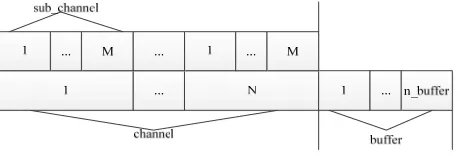
2) There are N channels in CRN, and each channel is

divided into M of the same sub-channel. Each PU occu-

pies a channel (that is M sub-channel), while each SU

only occupies a sub-channel. The buffer in CRN in our model is a different characteristic from some other studies, and a buffer denotes a sub-channel. For simplicity, we assume that the number of buffer ( ) is no less than M. This assumption is reasonable, because if

is less than M, the dropping probability of

SUs will be great because of the PUs’ coming. The sys-

tem model is showed in Figure 1.

_ n buffer

3) When a PU comes, if the number of PUs in CRN are less than N, the PU will be accepted, otherwise it will

be blocked, at the same time, if the channel chosen by PU is occupied by SUs, the SUs will monitor other idle channel to access or stay in buffer to wait for idle channel, if there is no idle channel in buffer, the SUs will be dropped. When a SU comes, if there is idle sub-channel, the SU will be accepted, otherwise it will be blocked.

4) The SUs in buffer is priority to the new coming SUs. When there is SUs in buffer, the new coming SUs will be rejected to access.

This paper, we consider the impact of the variable serving rate of system on performance of the system by using a Markov chain model, which will be introduced in part B in detail. The problem is described that the system adjusts its serving rate according to the current channel state information (CSI). That is when there are SUs in the buffer, the system will increase the serving rate, and the more the SUs in the buffer are, the faster the serving rate is. On the other hand, we will analyzed the impact of different number of buffer on the throughput of SUs, and then give the optimal number of buffer to maximize the throughput of SUs.

2.2. Markov-Chain Model

In this paper, the stochastic variables , and denote the number of active Pus, the number of active SUs and the number of SUs in buffer respectively at time t, where

( )

p

N t N ts( ) ( )

s B t

 



0,



,

 





p s

N t  N N t  0,N M , and

 

s

B t [0, _n buffer]. So we can derive the state vector

 

{ _p t ,N_s( ),t B t_s( )}, it denotes a state of Markov-

[image:2.595.310.540.631.709.2]

Chain at time t. Based on the above assumptions and analysis, the Markov-Chain model can be depicted in

Figure 1. In Figrue 1, we use {i, j, k} replace

{

S  N

 

,N t( ),B t( )

p s s

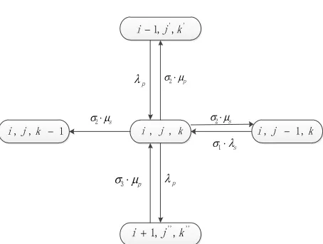
In Figure 2, the transition from state (i, j, k) to other

state, or from other state to state (i, j, k) occur with four

possible cases, i.e., PU arrival, PU departure; SU arrival, SU departure. And each state transition is with its corre- sponding rate. Taking an example of SU, when a SU arrives, the state (i, j-1, k) will be transferred to state (i, j, k) with the transition rate 1 s, in which 1

N t }.

σ λ σ 1 with the condition k = 0, otherwise σ10. When a SU

(3)

k j

i, ,

' ' ' '_, , 1j k i  1

,

,j k 

i i,j  1,k

' '_,

,

1j k

i

p

 2p

s

  2

s

 1

s

  2

p



p

[image:3.595.59.286.74.246.2]

 3

Figure 2. State transition of markov-chain model.

departures, the transition from state (i, j, k) to state (i, j-1, k) or state (i, j, k-1) with transition rate , where

and 2 s .

σ μ _ k n buf

2

σ  (1 k n buffer/ _ ) j j

'' 3

σ  (1 / fer)

'

, 0

k k 

In Figure 2, on the condition of

, and on the condition of

'_{ }

' _, '

j  j M k  k

kM M

_

M  k n buffer, as well as j' = j + k,

' _{_} _{, _} ₎

k （n bufferM n buffer

on the condition of . And the value of and are also depend on the value of k, when k = 0,

_

kn buffer j''

''

k

'' _, ''

j  j n k  k n

M

, 1,

, where nmax(0, ( 1)i M   j N ),

'' ''

else j  j M k, k + min ( _n bufferk M, ). Thereby, we set up all equilibrium equations for every state according to these arrows described above with eleven undetermined coefficients and (i = 1, 2; j

= 1, 2,…, 5) i

α βj

' ' '' ''

1 2 , ,

1 1, , 2 1, , 3

4 , 1, 5 , , 1

( p s p s) i j k

p _i _{j k} p _i _{j k} s s i j k s i j k

i j p

p p p

p p                             

i j k (1)

where: 1 2 1 2 3

1 ( ) 0

1 ( )

0 1 ( 0)

0

1 ( ) 0

1 ( 0) 0

if i N else

if i M j N M

else if i

else

i if i N

else if j else                                   4 5

1 ( )

0

( _ ) 0

j if i M j N M

else

j if k n buffer else                

Then, combining the normalized condition (2), we can get the steady state probability of each state.

, ,

0 0 0,

1

buffer

n N N M i M

i j k i j k i M j N M

p

  

      



 



(2)

With these steady state probabilities, we can evaluate the performance metric of the system, i.e., blocking probability, dropping probability, average handoff delay and throughput rate.

3. Performance Analysis and Algorithm

Description

3.1. Performance Analysis

1) The average handoff delay of SUs: SUs, which are being accepted service, are forced to switch to the buffer to wait for idle channel because of the arriving PU and no idle channel. The average time of staying in buffer is the average handoff delay, given in [7].

handoff buffer interference handoff

N N

Delay

N R

  (3)

where

handoff steady handoff

S S

S

N 



N P ,

denotes the average number of SUs which are forced to switch to the buffer when a PU comes, in which, S de-notes the state space and steady

S

P denotes the steady state

probability under the state S.

max(0, min( _ ,( 1) ))

handoff S

N  n buffer k i     M j N M ,

denotes, under the state S, the number of SUs which are

forced to switch to the buffer when a PU comes.

steady interference interference

S S

N 



N P , denotes the average number

of SUs which disturb to the new coming PU.

steady buffer

S S

N 



k P , denotes the average number of SUs

in the buffer.

handoff steady handoff

p

S S

S

R 



N  P , denotes the average rate of

switching to the buffer for SUs, i.e., the average number of switching to the buffer per unit time.

2) The blocking probability of Sus: When all channels are occupied, the coming SU will be blocked.

, , ,

block su

S i M j N M p

    





pi j k (4)

(4)

enoughchannels to accept the occupied SUs by PU, the occupied SUs will be dropped. First, we will consider the dropping probability of each SU:

 

, , max(0, 1

( _ ))

su

drop

i j k each

S

p p i M

j N M n buffer k



   

    



₍₅₎

So, to all SUs, the dropping probability is:

_

(1 )

drop p each su drop

su _block s su

p p

p



 

   (6) 4) The throughput rate of SUs: The SUs are not blocked and dropped.

(1 )(1 )

throughput block drop

su s su su

p    P p (7)

3.2. Algorithm Description

In the previous model, the numbers of buffer are equal to all the number of sub-channel. The only advantage of this model is no dropping probability, because the buffer can hold all the SUs which are occupied by PU. However, two disadvantages are resulted: one is that there are a lot of SUs in buffer, so the waiting time of SUs in buffer becomes long, i.e., the average handoff delay becoming long; the other one is that the author want to decrease the dropping probability to improve the throughput of SUs, but in fact, there are some SUs always stay in the buffer because of no idle channel being monitored, so the throughput of SUs may not be improved. In this case, we can decrease the numbers of buffer to decrease the average handoff delay of SUs, as well as not decreasing the throughput. However, there is a problem: how many buffers are optimal? Next, the algorithm of computing the optimal buffer for variable arrival rate of PUs in algorithm 1 will be presented.

Algorithm 1the computing of optimal n_buffer

for   p p1: pn;

for n buffer_ =1 : N M*



_



throughput;

su a n buffer p end

1

_ ( )p

n buffer  { n buffer_ | max(a[1],a[2] … a

[N M* ])}; end

1

_ [ _ ( ), , _p ( pn)]

n buffern buffer  n buffer _;

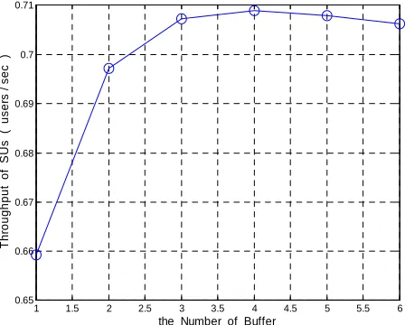
Taking an example，we give the parameters: N3, 2, p 1, p 1.5, s 0.8, s 0.4

M        

_

n buffer

, we can see the variation of the throughput of SUs with the variable

showing in Figure 3. When ≤4,

the throughput of SUs increase with the increasing of the number of buffer, while decrease when ≥4. The reason is that the more the number of buffer is, the more the average number of SUs in the buffer is, so the

less chance that the new SUs accepted will be, referring to the assumption (4), i.e., the higher the blocking prob-ability will be. On the other hand, although the dropping probability decrease with the increasing number of buffer, its value is so low that leads to the increasing of the total throughput. According to the analysis, we can get the optimal number of buffer is4 that can result the maximal throughput of SUs in this case.

_

n buffe

_

n buffe r

r

4. Simulation Result

In this section, we will evaluate each of the performance metrics analyzed above versus the variable arrival rate of PUs by simulation result. Let the parameters be:

3, 2, p 1.5, s 0.8, s 0.4

N M       ; the range of p is

from 0 to 1.0 and the step is 0.1. According to the de-scription of algorithm above, we have

_ [0, 2,3,3, 4, 4, 4, 4, 4, 4, 4]

n buffer

for each of p. For demonstrating our advantage, we

give the different simulation result for invariable service rate (IVSR) with _n buffer6, variable service rate (VSR) with _n buffer6 and variable service rate (VSR) with

_ uffer n_ ffer

n b  bu _{, where the} _{is a vector}

with the element of optimal number of buffer for differ-ent arrival rate of PUs.

_

[image:4.595.311.535.534.714.2]

n buffer

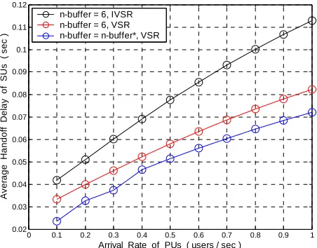
Figure 4 and Figure 5 show that as expected, the av-

erage handoff delay and the blocking probability of SUs increasewith increasing the arrival rate of PUs, because the numbers of idle channels decrease with increasing the traffic load of PUs, the accepted new SUs decrease and the number of SUs staying in buffer increase. However, as we expected, the average handoff delay and the blocking probability of SUs in VSR scheme decreases compared with IVSR. Furthermore, these two metrics also decrease in VSR scheme compared the maximal number of buffer ( _n buffer6) and the optimal number

1 1.5 2 2.5 3 3.5 4 4.5 5 5.5 6

0.65 0.66 0.67 0.68 0.69 0.7 0.71

the Number of Buffer

Th

roug

hput

of

SU

s (

user

s /

sec )

(5)

0 0.1 0.2 0.3 0.4 0.5 0.6 0.7 0.8 0.9 1 0.02

0.03 0.04 0.05 0.06 0.07 0.08 0.09 0.1 0.11 0.12

Arrival Rate of PUs ( users / sec )

Av

er

a

ge

H

a

nd

of

f

D

e

lay

of

SUs

( s

ec

)

[image:5.595.60.286.86.263.2]

n-buffer = 6, IVSR n-buffer = 6, VSR n-buffer = n-buffer*, VSR

Figure 4. Average handoff delay of SUs vs. arrival rate of PUs.

0 0.1 0.2 0.3 0.4 0.5 0.6 0.7 0.8 0.9 1 0

0.02 0.04 0.06 0.08 0.1 0.12 0.14

B

locki

ng

P

rob

ab

ili

ty

o

f S

U

s

[image:5.595.59.286.306.502.2]

Figure 5. Blocking probability of SUs vs. arrival rate of PUs.

of buffer ( ). The reason behind these results is that the faster the service rate is and the less the number of buffer is, the less the average number of SUs staying in buffer, so the waiting time in the buffer is less according to (4) and the blocking probability is lower, referring to assumption (4).

_ _

n buffer n buffer 

As is shown in Figure 6, when the number of buffer is

equal to all the sub-channels, i.e., the buffer can hold all the SUs occupied by the active PUs, there is no dropping probability for SUs, otherwise the dropping probability will be resulted due to the part of SUs being dropped by the arrival PU. From Figure 6, however, we know that

the maximal value of the dropping probability is still so low that it can fully satisfied the requirement of QoS, although the arrival rate of PUs is very high. In addition, several singularities in the left bottom correspond to

_ 2

n buffer and _n buffer3 in the vector of .

The last Figure 7 shows the curve of throughput of SUs

versus the arrival rate of the PUs. The trend of this variable confirms our analysis above.

_

n buffer

5. Conclutions

In this paper, we proposed a VSR scheme to optimize the average handoff delay of SUs, which is vitally important metric to real-time traffic, under the constraint of dropping probability for the CRN. Beside, we consider the case of buffer and give the algorithm for optimizing the number of buffer. Furthermore, the other performance metrics are also improved, and the simulation result demonstrates the feasibility and effectiveness of the new model. On the other hand, a little dropping probability which is met the requirement of QoS is lead, but we still want to reduce it as much as possible. So this is also our

0 1 2 3 4 5 6 7 8 9 10

0 0.5 1 1.5 2 2.5

3x 10

-3

Dr

opp

ing

Pr

obabi

lit

y

of

SU

s

Figure 6. Dropping probability of SUs vs. arrival rate of PUs.

0 0.1 0.2 0.3 0.4 0.5 0.6 0.7 0.8 0.9 1

0.68 0.7 0.72 0.74 0.76 0.78 0.8

Thr

oughp

ut

of

S

Us

( user

s

/ sec

)

[image:5.595.311.537.308.494.2] [image:5.595.311.538.534.717.2]

(6)

future work.

6. Acknowledgements

This work is supported by the National Natural Science Fund of China(No.61071068), the National High Tech- nology Research and Development Program of China (No. 2012AA121604), and theInternational S&T Pro- gram of China（No.2012DFG12010).

REFERENCES

[1] W. Lehr and L. W. McKnight, “Wireless Internet access: 3Gvs.WiFi?,” Telecommun. policy, Competition Wirel., Spectr., Service Technol. Wars, Vol. 27, No. 5/6, 2003,

pp. 351-370.

[2] M. A. McHenry, “NSF Spectrum Occupancy Measure-ments ProjectSummary,” Shared Spectrum Company Re-port, Aug. 2005.

[3] X. Zhu, L. Shen and T. P. Yum, “Analysis of Cognitive Radio Spectrum Access with Optimal Channel Reserva-tion,” IEEE Communications Letters, Vol. 11, No. 4, pp. 304-306, Apr. 2007.doi:10.1109/LCOM.2007.348282 [4] G. Liu, X. Zhu and L. Hanzo, “Dynamic Spectrum

Shar-ing Models for Cognitive Radio Aided Ad Hoc Networks

and Their Performance Analysis,” Proceeding of IEEE GLOBECOM 2011.

[5] E. W. M. Wong and C. H. Foh, “Analysis of Cognitive Radio Spectrum Access with Finite User Polulation,”

IEEE Communications Letters, Vol. 13, No. 5, 2009, pp.

294-296.doi:10.1109/LCOMM.2009.082113

[6] G. Liu, X. Zhu and L. Hanzo, “Impact of Variance of Heterogeneous Spectrum on Performance of Cognitive Radio Ad Hoc Network,” IEEE ICC, Vol. 1, No. 1, Jun

2012.

[7] Tumuluru, V.K.;Ping Wang; Niyato, D.and Wei Song, “Performance Analysis of Cognitive Radio Spectrum Access With Prioritized Traffic,” IEEE Transactions on Vehicular Technology, Vol. 61, No. 4, 2012, pp.

1895-1906. doi:10.1109/TVT.2012.2186471

[8] P. Zhou, Y. S. Chang and John A. Copeland, “Capacity and Delay Scaling in Cognitive Radio AdHoc Networks: Impact of Primary User Activity,” IEEE Globecom, 2010.

[9] W. T. Huang and X. B. Wang, “Throughput and Delay Scaling of General Cognitive Networks,” IEEE Infocom,

2011.

[10] N. Mokari, H. Saeedi and KeivanNavaie, “Channel Cod-ing Increases the Achievable Rate of the Cognitive Net-works,” IEEE Communications Letters, Vol. 17, No. 3,