Munich Personal RePEc Archive
Population-ageing, structural change and
productivity growth
Stijepic, Denis and Wagner, Helmut
FernUniversität in Hagen
15 February 2009
Population-Ageing, Structural Change and
Productivity Growth
by
Denis Stijepic (Corresponding Author) University of Hagen, Department of Economics Universitätsstr. 41, D-58084 Hagen, Germany Tel.: +49(0)2331/987-2640
Fax: +49(0)2331/987-391
E-mail: [email protected]
and
Helmut Wagner
University of Hagen, Chair of Macroeconomics Universitätsstr. 41, D-58084 Hagen, Germany Tel.: +49(0)2331/987-2640
Fax: +49(0)2331/987-391
E-mail: [email protected] Web: http://www.fernuni-hagen.de/HWagner
This version: February 2012
Abstract
Population-ageing is one of the traditional topics of development and growth theory and a key challenge to most modern societies. We focus on the following aspect: Population-ageing is associated with changes in demand-structure, since demand-patterns change with increasing age. This process induces structural changes (factor-reallocations across technologically heterogeneous sectors) and, thus, has impacts on average productivity growth. We provide a neoclassical multi-sector growth-model for analyzing these aspects and elaborate potential policy-impact channels. We show that ageing has permanent and complex/multifaceted impacts on the growth rate of the economy and could, therefore, be an important determinant of long-run GDP-growth.
Keywords: Population-ageing, demand shifts, reallocation of factors, cross-sector technology-disparity, GDP-growth, multi-cross-sector growth models, neoclassical growth models, structural change.
1. Introduction
Population-ageing – a term which in general refers to an increasing life span of an average member of a society – is one of the key stylized facts of the development process. It has had and will have some major impacts on economic and social structures in developing and industrialized economies. This fact is reflected by a large body of literature dealing with it. Well known examples of this literature are development and growth theories related to population growth, e.g. classical theories (like Malthusian development traps) and neoclassical growth theory (ranging from Solow-model to endogenous-growth theories), and most obviously theories of social security and pension systems. As well, these aspects are associated with actual policy making, including development policy (World Bank, UN, etc), population policy (e.g. in China), and major changes in pension and health systems in some industrialized economies. A very general discussion of population-ageing is provided by IMF (2004). The focus of our paper is on economic growth. (To some extent our paper has implications for pension systems as well). For an extensive discussion of models dealing with ageing and economic growth see, e.g., Gruescu (2007); for a short, but still very comprehensive, discussion see, e.g., Mc Morrow and Röger (2003). An overview of empirical studies is provided by, e.g., Groezen et al. (2005).
1.1 Focus of our paper
other words, ageing may induce “structural change” (i.e. cross-technology factor-reallocation), hence causing changes in aggregate (or: average) productivity growth. Thus, the increasing old-age pension payments (due to the increasing number of recipients) are confronted with changes in the growth rate of the tax-base, which may require changes in the old-age-pension system.
This line of arguments seems to be quite obvious, especially when thinking of services, like health care services and geriatric nursing services: in general, the “old” demand more of such services in comparison to the “young”; furthermore, the “production process” of these services is regarded to be technologically distinct (i.e. relatively labour-intensive) in comparison to e.g. manufacturing goods (see also IMF (2004), chapter 3, and especially p. 159). However, there are also some other differences in demand between the old and the young, e.g. the young have a relatively larger demand for commodities and investment goods (e.g. housing, car and furniture, i.e. things which the old may already have). Furthermore, in general, the old seem to spend a larger share of budget on services (see Groezen et al. (2005)).
1.2 Related empirical evidence
Empirical evidence on such differences in demand patterns between the old and the young and their growing importance (not only for factor reallocation across sectors) has been presented by, e.g., Börsch-Supan (1993, 2003), Fuchs (1998) and Fougère et al. (2007). Furthermore, empirical evidence implies that there are strong differences in technology across products/sectors (e.g. when comparing some services and manufactured products or health care services and commodities production): Evidence on differences in TFP-growth across sectors/products is provided by, e.g., Baumol et al. (1985) and Bernard and Jones (1996). Evidence on differences in capital intensities across sectors is provided by, e.g., Close and Schulenburger (1971), Kongsamut et al. (1997), Gollin (2002), Acemoglu and Guerrieri (2008) and Valentinyi and Herrendorf (2008). Nordhaus (2008) presents some evidence on the relevance of cross-sector reallocations for aggregate growth.1 Overall, this (partly indirect) evidence on
1
effects of ageing seems to provide sufficient incentive to take a look at their relevance from a theoretical perspective.
1.3 Related theoretical literature
Our model is related to the theoretical literature which postulates the importance of cross-sector technology-differences for GDP-growth, e.g. Baumol (1967) and Acemoglu and Guerrieri (2008). Baumol (1967) claims that cross-sector differences in (labour-)productivity-growth can cause (by themselves) a GDP-growth-slowdown via relative price changes (“Baumol’s cost disease”). However, Baumol (1967) does not analyze (ageing-induced) demand-shifts, and he makes as well some simplifying assumptions (e.g. he excludes capital accumulation), which may be not accurate for our goals as we will see later. Acemoglu and Guerrieri (2008) show that cross-sector differences in capital-intensities have an impact on aggregate growth. However, they as well do not include (ageing-induced) demand-shifts into their analysis. Furthermore, Rausch (2006) provides a two-sector Heckscher-Ohlin model with ageing, where ageing leads to an increase in the savings rate, since the old have relatively larger amounts of assets. He argues that ageing leads to changes in the relative sector-size (and, thus, in GDP-growth), provided that sectors differ by capital intensity (see Rausch (2006), pp. 20 ff.). He as well does not take account of the impacts of ageing-induced demand-shifts.
To our knowledge, the model by Groezen et al. (2005) is the only one which explicitly includes ageing-induced demand-shifts into analysis, where ageing is incorporated into a two-sector overlapping-generations model. The old consume the output of a “backward” services sector; this sector uses labour-input only and does not have any productivity growth. The young consume the output of a “progressive” commodities sector; this sector uses capital and labour as input factors and generates capital and endogenous technological progress which increases its productivity with time. Groezen et al. (2005) focus on the trade-off between the positive “savings-effect of longevity”2 and the negative
2
allocation-effects of ageing”3. They show the importance of the elasticity of substitution between capital and labour in the progressive sector. If this elasticity is equal to unity, the two effects offset each other and ageing has no impacts on growth in their model. However, if this elasticity is greater (smaller) than unity, ageing has a negative (positive) impact on growth.4
1.4 Model setup
In contrast to Groezen et al. (2005), we do not study the trade-off between “savings-effect” and “factor-allocation-effect”, but focus on a detailed and in some sense “more general” study of the “factor-allocation-effect”.5 We are able to provide a detailed discussion of the factor-reallocations and the “factor-allocation-effect (without simulations), because our paper is rooted in the “new” structural change literature, which is pioneered by Kongsamut et al. (1997, 2001), Ngai and Pissarides (2007) and Acemoglu and Guerrieri (2008). This literature focuses on neoclassical structural change modelling (capital accumulation and intertemporal utility maximization) and the usage of (partially) balanced growth paths (PBGPs). Especially, PBGPs facilitate the dynamic analysis significantly; see also the discussion in section 5.5.
Our model is a sort of disaggregated Ramsey-model6 where the representative household(s) consume(s) two groups of goods: “senior-goods” (i.e. goods which are primarily consumed by “older” people) and “junior-goods” (i.e. goods which are primarily consumed by younger people). Ageing (i.e. an increasing ratio of old-to-young) yields an increasing weight of senior-needs in the aggregate utility function, hence leading to a demand-shift in direction of senior-goods. We assume that the production of senior-goods and the production of junior-goods differ by TFP-growth and by capital-intensity (i.e. output-elasticity of inputs), according to the empirical evidence discussed above. Moreover, we include intermediates production into the model; this allows for linkages between senior- and junior-goods-production, which have been stated to be important by Fougère
3
The factor-allocation-effect has been described in section 1.1. In the Groezen-et-al.-(2005)-model this effect works as follows: ageing shifts factors to the “backward” services sector, since the “old” consume services only; thus, aggregate labour-productivity is lowered.
4
A paper, which is to some extent related to this topic, since it deals with ageing-related choice of technology, is provided by Irmen (2009).
5
In fact, the sort of “savings effect”, which is modelled by Groezen et al. (2005), does not exist in our model.
6
et al. (2007) and by Kuhn (2004); see also the discussion at the end of Section 2.2.
1.5 Model results
Overall, our results imply that the factor-allocation-effects of ageing on GDP-growth are “complex” (or: “multifaceted”), i.e. they are dependent on many parameters, consisting of several channels and potentially non-monotonous over time.
Furthermore, they seem to be very significant, from the theoretical point of view, since even a one-time increase in the old-to-young ratio causes permanent (non-transitory) impacts on the GDP-growth-rate. Thus, ageing seems to be an important determinant of GDP-growth.
For a more detailed summary of our results and their implications see section 5; especially, see section 5.4 for a comparison of our results to previous literature.
1.6 Setup of the paper
The rest of the paper is set up as follows: In sections 2 and 3 we present the assumptions and the solution of our model. In section 4 we analyze the impacts of ageing: first, we describe the dynamics of the equilibrium without ageing (section 4.1); subsequently, we compare this equilibrium to the equilibrium with ageing, where we present a simpler version of the model in section 4.2 (where only cross-sector-differences in TFP-growth exist) and the more sophisticated version of the model in section 4.3. Finally, we make some concluding remarks in section 5.
2. Model assumptions
2.1 Utility
We assume an economy where two groups of goods exist: “junior-goods” (goods m
(1)
∫
∞−
=
0
dt ue U ρt
where
(2) J uS
N L u
N L
u= +(1− )
(3) ⎥
⎦ ⎤ ⎢
⎣ ⎡
−
=
∏
=
m
i
i i J
i
C u
1
) (
ln θ ω
(4) ⎥
⎦ ⎤ ⎢
⎣
⎡ −
=
∏
+ =
n
m i
i i S
i
C u
1
) (
ln θ ω
(5a)
∑
∑
= = +
= =
m
i
n
m i
i i
1 1
0 ,
0 θ
θ
(5b)
∑
∑
= = +
= =
m
i
n
m i
i i
1 1
1 ,
1 ω
ω
(6) i N gL
L L g N N
i = =
∀ <
< 1 , & , &
0 ω
where Ci stands for consumption of good i and ρ is the time-preference rate. N
is an index of overall-population (including the young and the old) growing at constant exogenous rate; L is an index of the young (working) population growing at constant exogenous rate. Hence, the ratio L/N is an index of the share of the young as part of overall population, and a decreasing L/N can be interpreted as ageing.
The utility function is based on the Stone-Geary-preferences, where the θis can
be respectively interpreted as the subsistence levels (if θi > 0) or as levels of
home-production (if θi < 0). The income-elasticity of demand differs across goods; the price-elasticity of demand differs across goods as well and is not equal to unity. (See also Kongsamut et al (1997, 2001) for a discussion of a similar utility function.)
In this way we ensure that there are no other shifts in demand between the junior and senior sector, beside of those induced by ageing (a decreasing L/N): Provided that L/N is constant (no ageing), the demand for senior-goods and the demand for junior-goods grow at the same rate, yielding no factor reallocations between the senior- and the junior-sector. (Nevertheless, there are still demand shifts and reallocations within these sectors, due to the θis.)
Alternatively, the functions uJ and uS could be assumed to be of type Cobb-Douglas or CES. We chose Stone-Geary-preferences, since in this way we can add additional sources of demand-shifts (others than ageing) by omitting the restriction (5a) and (5b). This will be of importance later.
Note that there is a difference between demand-shifts which are modelled in standard structural change theory (e.g. in the paper by Kongsamut et al. (2001)) and ageing-induced demand shifts which are modelled in our paper. In standard structural change theory demand shifts are caused by differences in income-elasticity of demand across goods. Hence, some repercussions arise: changes in income -> demand shifts -> productivity impacts-> changes in income and so on. This repercussion does not arise in our model. In our model the chain of impacts is rather only in one direction: (income–independent) exogenous change in old-to-young ratio -> demand shifts -> productivity impacts -> change in income. Of course, one could postulate that changes in income are associated with changes in old-to-young ratio to some extent (e.g. due to improvement in medicine or do to some change in socio-cultural parameters which are associated with increasing income). This would imply that changes in the old-to-young ratio are endogenous. Although we believe that this is an interesting topic in general, a model with endogenous old-to-young ratio would yield very similar results as the standard structural change theory. The only difference would be that there is a further link
in the chain of impacts: income-change -> change in old-to-young ratio -> demand shifts -> productivity impacts -> income-change and so on.
arises due to some (from economist’s point of view) exogenous changes. For example, some socio-cultural parameters change (e.g. change in religiosity, emancipation) and/or some progress in medicine occurs independently of income level. Of course both factors depend on the income of a country to some extent; however, they must have some income-independent timely component.
Note that we are not the only ones, who model ageing as exogenous shifts in demand. For example, Groezen et al. (2005) model it in this way too. Overall, there seems to be a research gap in this field, which may be interesting to fill.
2.2 Production
According to the evidence discussed above, the senior-goods are not produced by the same technology as junior-goods; the technologies differ by TFP-growth and by output-elasticities of inputs (i.e. capital intensities differ between the senior- and the junior-sector). Furthermore, we assume that only the young supply labour on the market; hence L (and not N) is input in production:
(7) Yi = A(liL) (kiK) (ziZ) , i =1,...m
γ β α
(8) Yi = B(liL) (kiK) (ziZ) , i=m+1,...n
μ ν χ
(9) A gB
B B g A A
= = &
&
,
(10) 0<α,β,γ,χ,ν,μ <1; α +β +γ =1; χ +ν +μ =1
where Yi denotes the output of sector i; K denotes the aggregate stock of capital;
Z is an index of intermediate inputs; li,ki and zi denote respectively the fraction of labour, capital and intermediates devoted to sector i; A and B are exogenous technology parameters, where we assume that TFP-growth differs between the junior- and the senior-sector.
We assume that each sector’s output is consumed and used as intermediate input )
(hi ; only sector-m-output is used as capital:
(11) Yi =Ci+hi, ∀i≠m
where δ is the depreciation rate of capital. Provided that it is assumed that senior-goods are rather services, the assumption that only the junior-sector produces capital seems to be consistent with empirical evidence which states that nearly all capital goods are produced by the manufacturing sector (see e.g. Kongsamut et al. (1997, 2001)).
The intermediate-inputs-index (Z) is a Cobb-Douglas function of sectoral intermediate outputs (hi):
(13)
∏
∑
= =
= ∀
< <
= n
i i i
n
i
i i
h
Z i
1 1
1 ,
1 0
, )
( ε ε ε
This intermediate structure is the same as the one assumed by Ngai and Pissarides (2007). Note that it is important to assume intermediates production within this model. In general, we can assume that the old and the young consume many goods which are nearly the same. (However, the manner of consumption is quite different.) For example, the young and the old consume food. However, while probably many young cook the food by themselves, some very old consume the food by being served in retirement homes or hospitals. Hence, although the old and the young eat similar things, the share of services is larger in the consumption of the old. If we did not assume some intermediate linkages between the junior and senior consumption goods we would not take account for the fact that the old are the same human beings as the young (i.e. having the same basic needs). For example, the assumption that the old and the young consume different goods (which have no intermediate linkages) would e.g. imply that the old do not eat food. It would not be necessary to take account for these facts if intermediates production were irrelevant for the ageing-effects. However, as we will see, the output-elasticities of intermediate inputs determine among others the strength of the ageing impacts via structural change. Hence, we have to include intermediate linkages between senior-goods and junior-goods into our model.
All labour, capital and intermediate inputs are used in production, i.e.
(14)
∑
∑
∑
= =
=
= =
= n
i i n
i i n
i
i k z
l
1 1
1
1 ;
1 ;
2.3 Numéraire
Let pi denote the price of good i. We choose the output of sector m as numéraire. Hence,
(15a) 1pm=
It should be noted here that in reality real GDP is calculated by using an average price as GDP-deflator; i.e. in general, a basket of all goods which have been produced is used as numéraire. (See also Ngai and Pissarides (2007), p. 435, and Ngai and Pissarides (2004), p. 21.) We choose the manufacturing output as numéraire, since in this way we can analyze the equilibrium growth paths in the most convenient manner. Nevertheless, we will always calculate the GDP by using an average price deflator as well. We use the following compound deflator, which may be regarded as the theoretical mirror image of the deflators which are used to calculate real GDP in reality:
(15b)
∑
= ≡ n ii N
N i i
p Y
Y p p
1
where YiN and YN denote respectively the net-output of sector i and aggregate net-output. “Net-output” means here gross-output minus real value of intermediates inputs; thus, net-output is equal to “real-value added”. Hence, YiN is given by the following relation:
(15c) piYiN = piYi −ziH
net-output in our model can be seen in equation (A.25) from APPENDIX A and equations (16).)
Overall, our GDP-deflator (equation (15b)) is simply a weighted-average of prices, where we used outputs as weights. If we divide our aggregate net-output (expressed in manufacturing terms) by this deflator we have a GDP-measure which is similar to the one which is used in reality. However, all the issues regarding the choice of the numéraire are irrelevant when looking at shares or ratios (since the changes in the numéraire of the numerator offset the changes in the (same) numéraire of the denominator). For example, the
capital-to-output ratio (K/YN) is the same irrespective of the numéraire. (See also Ngai and Pissarides (2007), p.435 and Ngai and Pissarides (2004), p.21.)
2.4 Aggregates and sectors
We define aggregate (gross-)output (Y), aggregate net-output (YN), real GDP
(GDP), aggregate consumption expenditures (E) and aggregate value of intermediate inputs (H) as follows:
(16a)
∑
= ≡ n ii
iY
p Y
1
(16b) YN ≡Y −H
(16c)
p Y GDP≡ N
(17)
∑
= ≡ n i
i
iC
p E
1
(18)
∑
= ≡ n i
i
ih
p H
1
Throughout the paper we use aggregate net-output instead of aggregate (gross-)output (Y), since in general GDP does not include intermediates. (In our model Y is equal to the sum of investment, consumption and intermediates-value (H); see equation (A.25) in APPENDIX A.)
The aggregate input-shares of the junior-sector (lJ,kJ,zJ)and the aggregate
(19)
∑
∑
∑
∑
∑
∑
+ = + = + = = = = ≡ ≡ ≡ ≡ ≡ ≡ n m i i S n m i i S n m i i S m i i J m i i J m i iJ l k k z z l l k k z z
l 1 1 1 1 1 1 , , , , ,
The aggregate consumption expenditures on junior-goods (EJ) and senior-goods
)
(ES are given by:
(20)
∑
∑
+ = = ≡ ≡ n m i i i S m i i i
J pC E pC
E
1 1
S
E could also be interpreted as the budget devoted to the old. Throughout the paper we assume that the aggregate budget is distributed across the old and the young according to the representative household utility function (social welfare function). That is, budgets are such to maximize social welfare.
3. Model equilibrium
3.1 Optimality conditions
The model, as specified in the previous section, can be solved by maximizing life-time utility (equations (1)-(6)) subject to equations (7)-(15a), e.g. by using a Hamiltonian function. The intra- and intertemporal optimality conditions are (where we assume that there is free mobility of factors across sectors):
(21) i
h Z Z z Y Z z Y Z z Y K k Y K k Y L l Y L l Y p i m m i i m m i i m m i i m m i ∀ ∂ ∂ ∂ ∂ = ∂ ∂ ∂ ∂ = ∂ ∂ ∂ ∂ = ∂ ∂ ∂ ∂ = , ) ( ) ( / ) ( / ) ( / ) ( / ) ( / ) ( /
(22) i
C u C u p m i
i ∂ ∂ ∀
∂ ∂ = , / (.) / (.)
(23) −δ −ρ
∂ ∂ = −
) (k K
Y u u m m m m &
By using equations (1)-(20) these optimality conditions (equations (21)-(23)) can be transformed into the following equations (sections 3.2 and 3.3) describing the aggregate and sectoral behaviour of the economy (for a proof of these equations see APPENDIX A):
3.2 Aggregates
(24) K
c g g E
K
K L G
c m c
m ) ˆ
1 ( ˆ ˆ ) ( ˆ − + + − − +
=λ − α βλ δ
& (25) c g g K E E G L c c
m − − − − −
= − − 1 ˆ ˆ ˆ 1
1 δ ρ
βλ & (26a) αν χβ λ α χ β β α λ − − + −
= −c m
m
c v
K
Yˆ ˆ ( ) ( )
(26b) ˆ ˆc m c( m)
N K
Y = λ − α +βλ
(26c) α χ γε με λ αβ αν χβ β ν γε με λ S S c m c S S m K E N L + − ⎟ ⎠ ⎞ ⎜ ⎝ ⎛ − − − + − = − 1 ˆ ˆ 1 1 (26d) αν χβ λ αμ χγ β νγ βμ α λ − − + −
= −c m
m c K
Hˆ ˆ ( ) ( )
(27) 1 2 ) 1 ( ) 1 ( ) 1 ( ) ( ˆ ˆ − − ⎥ ⎦ ⎤ ⎢ ⎣ ⎡ − − − − − + +
= m m m S
c m c p K P D G αν χβ μ αβ λ βλ α βλ α λ
where 1
) 1 ( 1 ) 1 ( 0 < − − − + − ≡ < μ ε ε γ γν ε μ ε β S S S S c , m m m k l ≡
λ ,
∑
+ = ≡ n m i i S 1 ε ε , G G gG ≡ &
S S i S S S n i i B A G με ε γ γ ε ε μ ν χ ε γ με ε γ γ μ β ν α
χ − − −
= − ⎪⎭ ⎪ ⎬ ⎫ ⎪⎩ ⎪ ⎨ ⎧ ⎥ ⎥ ⎦ ⎤ ⎢ ⎢ ⎣ ⎡ ⎟⎟ ⎠ ⎞ ⎜⎜ ⎝ ⎛ ⎟⎟ ⎠ ⎞ ⎜⎜ ⎝ ⎛ ⎟ ⎠ ⎞ ⎜ ⎝ ⎛ ≡
∏
) 1 ( 1 1 1 , and[ ] (1 )
) ( 1 ) ( ) ( 1
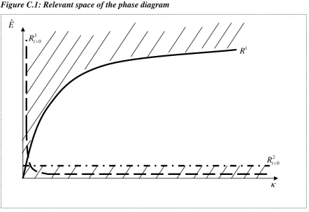
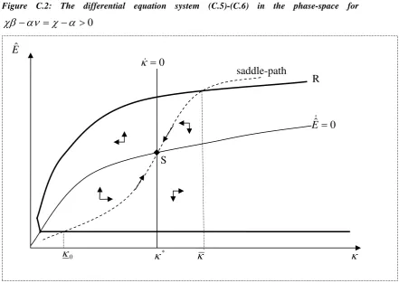
ˆ α ε γχ αμ
α χ ε μ γ γ αμ γχ ε α αν χβ μα γχ ε αμ αν αχ λ ε γ μ γ ν β χ
α − + − + −
Definition 1: Kˆ, Eˆ,Yˆ,GDˆP and YˆN stand for K,E,Y,GDPandYN expressed in “labour-efficiency-units, i.e. c LG Y Y − ≡ 1 1 ˆ , c LG K K − ≡ 1 1 ˆ , c LG E E − ≡ 1 1 ˆ , c LG GDP P D G − ≡ 1 1
ˆ and
c N N LG Y Y − ≡ 1 1 ˆ .
Note that this definition of variables in efficiency units makes our discussion about the equilibrium growth path easier later.
Proposition 1: p stands for the price of senior goods. S p is given by: S
[ ] (1 )
) ( 1 ) ( ) ( 1
ˆ α ε γχ αμ
α χ ε μ γ γ αμ γχ ε α αν χβ μα γχ ε αμ αν αχ λ ε γ μ γ ν β χ
α − + − + −
− + − − = ⎥⎥ ⎥ ⎦ ⎤ ⎢ ⎢ ⎢ ⎣ ⎡ ⎟⎟ ⎠ ⎞ ⎜⎜ ⎝ ⎛ ⎟⎟ ⎠ ⎞ ⎜⎜ ⎝ ⎛ ⎟⎟ ⎠ ⎞ ⎜⎜ ⎝ ⎛ ⎟ ⎠ ⎞ ⎜ ⎝ ⎛ ⎟⎟ ⎠ ⎞ ⎜⎜ ⎝ ⎛ ≡
∏
S S S i B A K p m n i i SProof: Remember that senior goods are produced by the same production functions; hence each senior good has the same price, pS. The rest of the proof is given in APPENDIX A. Q.E.D.
We can see that (beside of the GDP-measure) the optimum aggregate structure of this economy is quite similar to the optimum structure of the standard Ramsey-model (or sometimes also named “Ramsey-Cass-Koopmans Ramsey-model”).7 For a given
m
λ , equations (24)-(26b) determine the equilibrium savings rate of the model
(optimal intertemporal allocation of factors), like in the normal Ramsey-model. (In fact, for λm= 1 equations (24)-(26b) are the same as the corresponding
equations of the standard Ramsey-model). Equation (26c) determines λm as function of cross-sectors demand patterns (see also later equations (30) and (31)).
m
λ can be regarded as a productivity indicator of aggregate production: it
captures the changes in aggregate productivity which are caused by factor-reallocation across technologically distinct sectors (junior and senior sector), since λm depends only on the allocation of labour across the junior and senior
7
sectors: ⎟⎟ ⎠ ⎞ ⎜⎜ ⎝ ⎛ +
= J S
m l βχ l
αν
λ .8 Furthermore, equation (26c) determines the λm
which is consistent with the efficient (intratemporal) allocation of factors across sectors, since equation (26c) can be derived from equations (14) and (21) (among others); see as well the derivations in APPENDIX A. (Equations (14) state that all factors must be used in production, i.e. no factors are wasted; equation (26c) requires that marginal rates of technical substitution are equal across sectors, i.e. factors are efficiently allocated across sectors.)
3.3 Sectors
(28) ) ( ) ( ) ( αν χβ λ α χ β ν β α δ ε − − + − ⎟⎟ ⎠ ⎞ ⎜⎜ ⎝ ⎛ + + + = m J J J Y K K Y H Y E l & (29) α χ αν χβ λ α χ β ν β α ε ) ( ) ( ) ( − − + − ⎟ ⎠ ⎞ ⎜ ⎝ ⎛ + = m S S S Y H Y E l (30) N L E EJ =(31) ⎟
⎠ ⎞ ⎜ ⎝ ⎛ − = N L E ES 1
(32a) m m i i l k l k χβ αν
= for i=m+1,...n
(32b) i
m m
i l
l k
k = for i=1,...m
(33a) m m i i l z l z χγ αμ
= for i=m+1,...n
(33b) i
m m
i l
l z
z = for i=1,...m
where
∑
= ≡ m i i J 1 ε ε .
For a proof of these equations see APPENDIX B.
We can see that ageing (i.e. changes in L/N) induces demand shifts between the junior- and the senior-sector (equations (30) and (31)). These demand shifts lead
8
to changes in factor allocation between these two sectors (here shown by changes in employment shares; see equations (28) and (29)). Further factor-reallocation between the senior- and the junior-sector is caused by changes in aggregate capital demand (since only the junior-sector produces capital) and by changes in aggregate intermediates demand.
Proposition 2: Capital intensity in the senior sector ( L l
K k
S S
) is lower in
comparison to capital-intensity in the junior sector ( L l
K k
J
J ), provided that
χβ
αν < (αμ<χγ). Intermediate-intensity in the senior sector ( L l
Z z
S
S ) is lower
in comparison to intermediate-intensity in the junior sector ( L l
Z z
J J
), provided that
χβ
αν < (αμ<χγ).
Proof: Since capital intensity in a subsector i is given by i L l
K k
i
i ∀
, , and
intermediates intensity in a subsector i is given by i L l
Z z
i
i ,∀ , equations (19), (32)
and (33) imply this proposition. Q.E.D.
4. Effects of ageing
To study the effects of ageing we compare the economy without ageing (L/N = constant) to the economy with ageing (L/N decreases), ceteris paribus. In all the
following argumentation, ageing (i.e. a change in L/N or a change in N
L N−
)
(Working)Definition 2: Ageing stands for an increase in N/L, where gL is constant.
In the next section (4.1) we discuss the equilibrium without ageing. In section 4.2, we analyze the effects of ageing in a simpler version of our model, where only cross-sector-differences in TFP-growth are allowed for. In section 4.3 the effects of ageing are analyzed in the general version of the model, where it is allowed for cross-sector differences in input-elasticities as well.
4.1 Partially Balanced Growth Path (PBGP) without ageing
In this subsection we assume that there is no ageing, i.e. L/N = constant.
Definition 3: A “partially balanced growth path” (“PBGP”) is an equilibrium
growth path where Kˆ, Eˆ,Yˆ,YˆN and λm are constant.
The name “partially balanced growth path” reflects the fact that along the PBGP some variables (Y,K,E andYN) behave as if they were on a balanced growth path (steady state), while the other variables (e.g. GDP) do not behave in this manner, i.e. they grow at non-constant rates, as we will see soon. (This concept is similar to the concept of “aggregate balanced growth”, which is used by Ngai and Pissarides (2007).)
Lemma 1: There exists a unique PBGP of the dynamic equation system (24)-(26),
provided that L/N is constant.
Proof: It can be seen at first sight that equations (24)-(26) imply that there is an equilibrium growth path where Kˆ, Eˆ,Yˆ,YˆN and λm are constant, provided that L/N is constant. Q.E.D.
Lemma 2: Along the PBGP, the growth rate of the variables Y,K,E andYN is
given by
(34) .
) 1 (
) 1 (
* g g g const
g L
S S
B S A
S + =
+ −
+ −
=
χ γε α με
(where L/N is constant).
Proof: This lemma is implied by Definitions 1 and 3. Q.E.D.
Lemma 3: Along the PBGP, factors are not shifted between the senior- and the
junior-sector, i.e. l and J l are constant, (where L/N is constant). S
Proof: This lemma is implied by equations (28)-(31), by Definitions 1 and 3 and by Lemma 2. Q.E.D.
Definition 4: An asterisk (*) denotes the PBGP-value of the corresponding variable.
Now, we derive the PBGP-values of variables as functions of exogenous parameters:
Lemma 4: Along the PBGP, the variables Kˆ, Eˆ,Yˆ,YˆN,GDˆP and λm are given by the following functions of exogenous model parameters (where L/N is constant)
(35a) 1 * 1 * ˆ m c s K = − λ
(35b) 1 *
1 1 * ˆ m c c c s s
E =α − +ρ − λ
(35c) αν χβ λ α χ β β α − − + − = − * 1 * ( ) ( )
ˆ c m
c
v s
Y
(35d) ˆ* 1 ( * ) m c
c
N s
Y = − α+βλ
(35e) s N L N N L N S S m β ρ αν χβ ε μα χγ α αν χβ ε μβ νγ β β α λ − − + − + − − − − + = ) ( ) ( ) ( ) ( * (35f) 1 * * * 2 * 1 * ) 1 ( ) 1 ( ) 1 ( ) ( ˆ − − ⎥ ⎦ ⎤ ⎢ ⎣ ⎡ − − − − − + +
= c m m m S
(35g)
[ ] (1 )
) ( 1
) ( ) (
1 1
1
*
αμ γχ ε α
α χ ε
μ γ γ
αμ γχ ε α αν χβ μα
γχ ε αμ
αν αχ
ε γ μ γ ν β χ
α − + − + −
− + − − −
= ⎥⎥
⎥
⎦ ⎤
⎢ ⎢ ⎢
⎣ ⎡
⎟⎟ ⎠ ⎞ ⎜⎜ ⎝ ⎛ ⎟⎟ ⎠ ⎞ ⎜⎜
⎝ ⎛ ⎟⎟ ⎠ ⎞ ⎜⎜ ⎝ ⎛ ⎟ ⎠ ⎞ ⎜ ⎝ ⎛ ⎟⎟ ⎠ ⎞ ⎜⎜ ⎝ ⎛
=
∏
S S
S
i
B A s
p c
n
i i S
(35h)
c g g s
G
L + −
+ + ≡
1
ρ δ
β
.
Proof: To determine the PBGP-values of Kˆ, Eˆ,Yˆ,YˆN and λm we have to set
0 ˆ =
K& and Eˆ& =0 (because of Definition 3). Then equations (24)-(27) imply Lemma 4. Remember that in this section L/N is constant. Q.E.D.
Lemma 5: The young-to-old ratio ( N L
) has an impact on the PBGP-levels of
aggregate variables Kˆ*, Eˆ*,Yˆ*,YˆN*,GDˆP* and
*
m
λ (where L/N is constant).
Proof: This lemma is implied by equations (35). Q.E.D..
Lemma 6: GDˆP* does not grow at constant rate along the PBGP (even when N/L is constant).
Proof: This lemma is implied by (35f). Note that equation (35g) implies that pS*
is not constant along the PBGP. Q.E.D.
Lemma 6 shows a quite convenient feature of our model: we can study the rich dynamics of the GDP (where the reallocation-effects of ageing cause unbalanced-growth of GDP) while the other variables are on a (partially) balanced unbalanced-growth path (partial steady state). This fact makes it possible to analyze the impacts of ageing without simulations.
Lemma 7a: A saddle-path, along which the economy converges to the PBGP,
exists in the neighbourhood of the PBGP of the dynamic equation system (24)-(26).
Lemma 7b: If intermediates are omitted (i.e. if γ =μ =0), the PBGP of the dynamic equation system (24)-(26) is locally stable.
Corollary 1: Even if the initial capital level is not given by equation (35a), the
economy which is described by the aggregate equation system (24)-(26) converges to the PBGP, provided that L/N is constant.
Proof:This corollary follows from Lemmas 1, 4 and 7. Q.E.D.
4.2 Ageing and cross-sector differences in TFP-growth
In this subsection we provide a simpler version of our model, which is helpful to understand the general mechanism which leads to the reallocation effects of ageing. We assume now that input-elasticities are equal across sectors, i.e.
ν β χ
α = , = and, thus, γ =μ. Furthermore, we assume that ageing takes place.
Lemma 8: If α =χ, β =ν and, thus, γ =μ, equations (24)-(35) become:
(24)’ K
c g g E K K G L c ˆ ) 1 ( ˆ ˆ ) ( ˆ − + + − − +
= α β δ
& (25)’ c g g K E E G L c − − − − − = − 1 ˆ ˆ ˆ
1 δ ρ β
&
(26a)’ Yˆ =Kˆc
(26b)’ YˆN =Kˆc(α+β)
(26c)’ λm =1
(26d)’ Hˆ =Yˆ−YˆN =γYˆ
(27)’ 1 1 ) ( ˆ ˆ − ⎥⎦ ⎤ ⎢⎣ ⎡ − + + = B B A l K P D
G c α β S
(28)’ ⎟⎟
⎠ ⎞ ⎜⎜ ⎝ ⎛ + + + = Y K K Y H N L Y E
lJ J
δ ε &
(29)' ⎟⎟
⎠ ⎞ ⎜⎜ ⎝ ⎛ + ⎟ ⎠ ⎞ ⎜ ⎝ ⎛ − = S S Y H N L Y E
l 1 ε
(34)' S A S B L
g g g
g = − + +
α γε γε ) 1 ( *
(35a)’ K =s1−c
1 *
ˆ
(35b)’ c c
c s s
E = − + 1− 1 1
*
(35c)’ c c
s Yˆ* = 1−
(35d)' ˆ* = 1−c(α+β) c N s Y (35f)' 1 1 * 1 ) ( 1 ) ( ˆ − − ⎭ ⎬ ⎫ ⎩ ⎨ ⎧ ⎥ ⎦ ⎤ ⎢ ⎣ ⎡ + ⎟ ⎠ ⎞ ⎜ ⎝ ⎛ − + − + + = S c c N L s B B A s P D
G α β α ρ γε
where 0 <1 + = < β α β c , β α β α ε ε β
α γ ε +
− − = + ⎪⎭ ⎪ ⎬ ⎫ ⎪⎩ ⎪ ⎨ ⎧ ⎥⎦ ⎤ ⎢⎣ ⎡ ≡
∏
1 1 1 n i i i S A B A G .Proof: The proof is quite straight-forward. Therefore, we omit it here. Note that following steps are necessary to obtain equation (27)’: By inserting equation (26c) into equation (27) the following equation can be obtained:
[
]
12 ) 1 )( 1 ( / 1 ) / ˆ /( ˆ / ) ( ) ( ˆ ˆ − − ⎥ ⎦ ⎤ ⎢ ⎣ ⎡ − − + − − − − + + = S S S c m S m m c m c p K E N L N K P D G μ α χ γε με λ γε βλ α βλ α λ
This term can be reformulated by using the other equations to obtain
[
]
[
]
1) / 1 ( ˆ / ˆ / ) ( 1 ) ( ˆ
ˆP=K + − + N−L N E Y −A B −
D
G S
c α β γε
. Then, by using equations (26d)’ and (29)’, equation (27)’ can be derived. Q.E.D.
Lemma 9: If input-elasticities are equal across sectors, there exists a unique
PBGP, irrespective of whether ageing takes place or not, and irrespective of the rate of ageing.
Proof: Lemma 8 implies that equations (24)’-(26)’ apply here. The proof of Lemma 9 can be seen directly from equations (24)’-(26c)’, which are nearly the same as in the standard one-sector Ramsey model. Since equations (24)’-(26)’ are not dependent on L/N, the existence of the PBGP is not affected by changes in L/N. Q.E.D.
Lemma 10: If input-elasticities are equal across sectors, the growth rate of the
variables Y,K,E, andYN is given by equation (34)’ along the PBGP.
Lemma 11: If input elasticities are equal across sectors, the PBGP is globally
saddle-path stable, irrespective of whether ageing takes place or not.
Proof: Lemma 8 implies that equations (24)’-(26)’ apply. Equations (24)’ and (25)’ are the same as in the standard Ramsey-model regarding all relevant features. Therefore, the aggregate system of our model behaves like the standard Ramsey-model, i.e. it is globally saddle-path stable. (See also Ngai and Pissarides (2007) on the stability of such frameworks.). Since equations (24)’-(26)’ are independent of L/N, ageing has no impact on the stability of the PBGP. Q.E.D.
Corollary 2: When input-elasticities are equal across sectors, ageing is irrelevant
regarding the development of the variables Y,K,E, andYN in our model: Neither
the PBGP-growth rate g nor the PBGP-levels * Kˆ*, Eˆ*,Yˆ*andYˆN* are affected by (the level or the growth rate of) L/N. A change in L/N does not induce a
deviation from the (initial) PBGP with respect to Y,K,E, andYN.
Proof: This corollary is implied by Lemmas 8-10 and equations (35). Q.E.D.
Now we take a look at the disaggregated variables of the economy.
Theorem 1: If input-elasticities are equal across sectors, ageing shifts demand from the junior-sectors to the senior-sectors along the PBGP. That is, decreases
in L/N lead to decreases in EJ/E and increases in ES /E.
Proof: This theorem is implied by equations (30) and (31). Remember that, as argued in section 2, the choice of the numéraire is irrelevant when looking at shares or ratios. Q.E.D.
Theorem 2: If input-elasticities are equal across sectors, ageing reallocates factors from the junior-sectors to the senior-sectors along the PBGP; i.e.
decreases in L/N lead to decreases in l and increases in J l .S
Proof: This theorem is implied by Lemma 8 and equations (28)’ and (29)’.
Q.E.D.
Theorem 3: If input elasticities are equal across sectors, ageing reduces the
TFP-level) is lower in the senior sector in comparison to the junior sector. That is, a decreasing L/N causes a reduction of the GDP-growth rate, provided that
A>B and gA >gB.
Proof:This theorem is implied by Lemma 8 and equation (35f)’. Q.E.D.
Corollary 3: If input-elasticities are equal across sectors, ageing shifts demand
from the junior-sectors to the senior-sector. These demand shift cause factor reallocation from the junior-sector to the senior-sector. This reallocation process reduces the growth rate of GDP provided that the senior-sector has a relatively low TFP(growth-rate) in comparison to the senior sector.
Proof: This corollary is implied by Theorems 1-3. Q.E.D.
Hence, whether ageing increases or decreases the GDP-growth-rate depends only on the TFP-relation between the junior and senior sectors. The factors which determine the strength of the ageing-impact are analyzed in the next section.
As argued in section 2, the choice of the numéraire is irrelevant when looking at shares or ratios. Hence, we can analyze the senior-goods-consumption-to-output ratio (ES /YN) without worrying about numéraire choice. The share of
senior-budget in aggregate output (ES /YN) increases at the same rate as the
old-to-young ratio (see equation (31) and remember that along the PBGP E and YN grow at the same rate).
All the results from this section are valid for the case that the budget devoted to seniors (e.g. old age pensions) develops according to the social welfare function (representative household utility function). If however political issues led to a reduction of old age pensions, the ageing-impacts would be weaker. We will discuss this case later.
4.3 Ageing and cross-sector differences in
input-elasticities
this paper we analyze only the case where the capital intensity in the senior sector is lower in comparison to the junior sector (i.e. αν <χβ ), since this case is in general assumed in the literature (see also Proposition 2). We assume that initially the economy is in the equilibrium described in section 4.1 with L/N = constant. In sections 4.3.1 and 4.3.2 we analyze what happens if there is a one time decrease in L/N (according to Definition 2). (After this decrease L/N is constant again.) In section 4.3.3 we generalize our results to the case where L/N increases consecutively. Furthermore, in section 4.3.1 we analyze the effects of ageing on net-output and on the pension-to-output ratio and we derive the impact channels, whereas in section 4.3.2 we look at the differences in this analysis when our GDP-measure is taken into account.
4.3.1 Productivity effect: Impacts and channels
In this subsection the term “aggregates” refers only to Y,YN,E and K but not to GDP.
Lemma 12: A one time decrease in L/N leads to a change of the PBGP. That is, the economy leaves the old PBGP and there is a transition period where the
economy converges to the new PBGP. The growth rate of aggregates (g ) is the *
same along the old and the new PBGP.
Proof: Remember that we assume here again that the input-elasticities differ across sectors; hence equations (24)-(35) apply here. Equations (35) imply that there must be a transition period, since the old and the new PBGP require different equilibrium capital levels; i.e. K* depends on L/N. (That is, the capital level which exists when the decrease in L/N occurs is not the same as the capital level which brings the economy directly on the new PBGP; we know from the discussion of the standard one-sector Ramsey-model that this induces a transition period, where the economy is converging to the new PBGP.) Furthermore, Lemma 7 and Corollary 1 imply that the economy will converge to the new PBGP (provided that the decrease in L/N is not too strong). Equation (34) implies that the growth rate of aggregates (g*) is the same along the old and the new PBGP,
Lemma 13: A one-time decrease in L/N reduces the growth rate of aggregates
during the transition period between the old and the new PBGP. That is, the
growth-rate of aggregates (K,E, andYN) during the transition period is lower in
comparison to the growth rate of aggregates along the (old and new) PBGP (g ). *
Proof: To prove this lemma we need the following derivatives of equations (35). (Note that our key results would not change, if we calculated here elasticities instead of derivatives.)
(36a) ˆ 1 0
1 * * > = ∂
∂ −c
m s K
λ
(36b) ˆ 1 0
1 * * > = ∂
∂ −c
m s E ρ λ (36c) αν χβ α χ β λ − − = ∂
∂ˆ 1− ( )
* * c c m s Y
(36d) ˆ 1 0
* *
> =
∂
∂ −cc
m
N s
Y β
λ
(36e) 0
) ( ) ( ) ( ) ( ) ( 2 * < ⎥ ⎦ ⎤ ⎢ ⎣ ⎡ − − + − + − + + − + − − = ⎟ ⎠ ⎞ ⎜ ⎝ ⎛ − ∂ ∂ s N L N s s N L N S S S m β ρ αν χβ ε μα χγ α β ρ ε μβ γν ρ ε μα χγ α β α αν χβ λ
From these equations we can see that a one-time decrease in L/N leads to a decrease in λ*m. The decrease in λ*m leads to a decrease in Kˆ*, Eˆ* ,andYˆN*.9
Hence, the values of Kˆ*, Eˆ*,andYˆN* along the new PBGP are lower in comparison to those of the old PBGP. Therefore, we can conclude that
* * * ˆ and , ˆ , ˆ N Y E
K decrease during the transition period. Hence, the growth rate of
aggregates (K,E and YN) during the transition period is lower than
*
g . (Remember that Definitions 1 and 3 and Lemma 2 imply the following: if
* * * ˆ and ˆ , ˆ N Y E
K are constant, aggregates (K,E and YN) grow at the constant rate
9
*
g ; hence, if Kˆ*,Eˆ*and YˆN* decrease, the growth rate of K,E and YN is lower
than g*. Note that this argumentation works, since “efficiency units” are the same along the old and the new PBGP: We express the variables in efficiency units (see
Definition 1) as follows: e.g.
c LG
Y Y
− ≡
1 1
ˆ ; since LG1−c
1
does not change due to
ageing, efficiency units are the same along the old and the new PBGP.) Q.E.D.
We will discuss the intuition behind this lemma soon; at first we postulate two lemmas, which are helpful to understand Lemma 13.
Lemma 14: A one-time decrease in L/N shifts demand from the junior-sector to
the senior-sector. That is, along the new PBGP E ES
is higher ( E EJ
is lower) in
comparison to the E ES
( E EJ
) of the old PBGP.
Proof: This lemma is implied by equations (30) and (31). Q.E.D.
Lemma 15: A one-time decrease in L/N leads to factor reallocation from the
junior-sector to the senior-sector. That is, along the new PBGP l is higher in S
comparison to the l of the old PBGP. S
Proof: By using equation (A.23) from APPENDIX A, it can be shown that the
employment share along the PBGP is given by
αν χβ
χβ λ
− −
=(1 *)
*
m S
l . Since
equation (36e) implies that 0 1
* < ⎟ ⎠ ⎞ ⎜
⎝ ⎛ − ∂
∂
N L m
λ
, a decrease in L/N leads to a decrease in
*
m
λ . Therefore, lS* increases due to a decrease in L/N. (Remember that we
assume that χβ −αν >0.) Q.E.D.
in comparison to the (junior-sectors). This is reflected by the fact that optimal capital intensity in the senior-sector is lower in comparison to the junior-sector (see Proposition 2). Hence, the ageing-induced (one-time) demand-shift implies that aggregate capital becomes less productive when looking at the economy-wide-averages. Therefore, at the aggregate level a one-time decrease in L/N acts similarly like a negative productivity-shock (a decrease in the productivity of capital).10 This leads to the negative impacts on aggregate net-output-growth, aggregate capital-growth and aggregate consumption-expenditures-growth (and of course, the savings rate decreases, since savings which are invested in capital become less rentable, i.e. the opportunity costs of consumption decrease). This adjustment-process occurs during the transition period. Since a one-time productivity-level-shock has no impacts on productivity-growth rates, the economy converges to a growth path (PBGP) where the growth rate is the same as before. (Remember that steady state growth rates are determined only by productivity-growth and not by productivity-levels within the standard (one-sector) Ramsey-model; in this respect our aggregate model is the same as the standard Ramsey model.)
A further interesting question is about the effects of ageing on the senior-budget-to-the-net-output-ratio (ES /YN). Equations (31), (35b) and (35d) imply the following derivative (consider also equation (36e)):
(37) 0
1 )
( ˆ
ˆ ) ˆ / ˆ (
2 * *
* * * *
> ⎟ ⎠ ⎞ ⎜
⎝ ⎛
− + + +
−
⎟ ⎠ ⎞ ⎜
⎝ ⎛ − ∂
∂ − = ⎟ ⎠ ⎞ ⎜
⎝ ⎛ − ∂ ∂
c g g s N
L N
N L N Y
E
N L N
Y
E G
L m
m
N N
S δ
βλ α
α λ
Hence, we can see that ageing increases the senior-budget-to-output-ratio. The first term on the right-hand-side of equation (37) may be regarded as the direct effect of ageing (i.e. an increase in the old-to-young ratio, increases the share of the seniors in the overall consumption-to-output-share).11 The second term may be regarded as an indirect effect: the increase in the old-to-young ratio leads to an
10
This fact is reflected by the ageing-induced decrease in λ*m, which is implied by equation (36e); as discussed in section three λ*m can be interpreted as a productivity indicator, which reflects the aggregate impacts of cross-sector factor-reallocation.
11
increase in the overall consumption-to-output-share12 (i.e. as noted above the savings-rate decreases due to lower productivity level).
We can see from equations (36) and (37) that a rich “portfolio” of parameters determines the strength of the impact of ageing. (Note that this portfolio would not change, if we calculated elasticities instead of derivatives in equations (36) and (37).) These parameters are:
a) technology parameters: input-elasticities of sectoral production functions (including labour, capital and intermediates elasticities), TFP-growth-rates (via
G
g ) and the depreciation rate b) time preference rate
c) old-to-young ratio and the growth rate of labour.
The reason for the fact that so many parameters determine the impact of ageing is the following: The demand-shift across technologically distinct sectors makes it necessary to change the (average) aggregate structure of the economy, especially the ratios between aggregate capital, labour and aggregate intermediates. The sectoral technology parameters (especially the input-elasticities) determine how strong this change has to be. Furthermore, since changes in capital in general
require an adjustment of the savings rate (
* *
ˆ ˆ 1
Y E
− ), all the variables which
determine the savings rate come into account, especially the parameters captured by the auxiliary variable s; see equations (35), e.g. the time-preference rate. The portfolio of parameters which determine the savings rate includes all those parameters which are already known to determine the savings-rate of the standard Ramsey-model (see the auxiliary variable “s”). However, our model provides a sector foundation of those parameters: especially, gG and c are assumed to be exogenous in the standard Ramsey-model, while in our model these two variables are functions of sectoral parameters.
12
since
(
)
(
)
01 )
( / ) ( /
) (
) ˆ / ˆ (
2 * *
* *
> ⎟ ⎠ ⎞ ⎜
⎝ ⎛
− + + +
− ∂
∂ − = −
∂ ∂
c g g s N
L N N
L N
Y
E G
L m
m
N δ
βλ α
α λ
4.3.2 Additional impacts on GDP: The price-effect
Remember that we have shown in the previous section that a one-time increase in L/N leads to a transition from the old PBGP to a new PBGP. Due to this fact, the effect of ageing on real GDP-growth can be divided into transitional effects and PBGP-effects. Transitional effects have an impact on the real GDP-growth-rate during the transition between two PBGPs, while PBGP-effects of ageing have an impact on the growth rate along the new (PBGP). In fact we have shown that the effects from the previous section are transitional. In this section we will introduce a new effect which affects real GDP-growth (but not the growth rate of other aggregate variables). We name this effect price effect, and we show that this effect is not only transitional.
4.3.2.1 Transitional effects of ageing on GDP
To show these facts we have to calculate the derivative of equation (35f): (38) ⎥ ⎥ ⎥ ⎥ ⎦ ⎤ ⎢ ⎢ ⎢ ⎢ ⎣ ⎡ ⎟⎟ ⎠ ⎞ ⎜⎜ ⎝ ⎛ + − − − − − ⎟⎟ ⎠ ⎞ ⎜⎜ ⎝ ⎛ − − + + ′ = ⎟ ⎠ ⎞ ⎜ ⎝ ⎛ − ∂ ∂ + + − − 4 4 4 4 8 4 4 4 4 7 6 4 4 4 8 4 4 4 7 6 4 4 8 4 4 7
6 ( )
* * ) ( * ) ( * 2 * * 1 * 1 ) 1 ( ) 1 ( ) ( ) ( ) ( ˆ χ αν χβ γ μ χ αν β β α βλ α λ β S S S m m c c l p l p s N L N P D G where ⎟ ⎠ ⎞ ⎜ ⎝ ⎛ − ∂ ∂ ≡ ′ N L N m m * * )
(λ λ , 1 (1 ) 1 *(1 *)
* * S m m p p − + − − − − = βλ α λ αν χβ μ αβ and αν χβ χβ λ − −
=(1 *)
*
m S
l .
and where pS* is given by equation (35g).
(For an explicit proof see APPENDIX D.) A “(+)” (a “(-)”) above a term denotes that this term is positive (negative).
senior goods are “more expensive” in comparison to junior-goods; i.e. provided
that pS* >1, where pS* is given by equation (35g).
Proof: This theorem is implied by equation (38). If pS* >1, an increase in the
old-to-young-ratio has a negative impact on the GDˆP*-level (and hence a negative impact on the GDP-growth-rate during the transition period; see also the argumentation in the proof of Lemma 13). Note that pS* is always positive and determined by exogenous parameters. Furthermore, note that the relative price of senior goods is given by pS* (see proposition 1) and the price of junior goods is given by 1. The latter comes from the fact that sector m is numéraire (see equation (15a)) and belongs to the junior-sector and all junior sub-sectors have identical production functions (see also equations (A.5) and (A.6) in APPENDIX A). Q.E.D.
If pS*<1, the effect of an increase in the old-to-young ratio may be positive or
negative, depending on the parameter constellation, where the effect can be positive provided that pS* is relatively small (i.e. relatively close to zero). To isolate the set of parameter-values which ensures that the GDP-effect of ageing is positive when pS* is relatively close to zero, we have to calculate the limit-value of the term within the squared brackets of equation (38), i.e.
(39)
⎟⎟ ⎠ ⎞ ⎜⎜
⎝
⎛ −
− − − +
=
⎥ ⎥ ⎦ ⎤ ⎢
⎢ ⎣ ⎡
⎟⎟ ⎠ ⎞ ⎜⎜
⎝ ⎛
+ − − −
− − ⎟⎟ ⎠ ⎞ ⎜⎜
⎝ ⎛
− − + →
*
* *
* 0
) (
2 ) ( ) (
1 ) 1 )( 1
( lim
S
S S
S p
l
l p
l
S
αν χβ
αν α
β χ β α
χ αν χβ
γ μ
χ αν β β α
where
αν χβ
χβ λ
− −
=(1 *)
*
m S
l .
If (39) is negative, equation (38) implies that for small values of pS* the effect of ageing is positive regarding GDP-growth. Equation (39) implies that, e.g., β <α is a stronger than necessary condition for this. (Remember that we assume that
Now, the question is what parameter constellations ensure that pS* is relatively small.
Lemma 16: In the limit pS* >1 (pS*<1), provided that the growth rate of labour-augmenting technological progress in the junior-sector is higher (lower) in comparison to the growth rate of labour-augmenting technological progress in
the senior-sector, i.e. provided that gA gB
χ α
1 1 >
( gA gB
χ α
1 1 <
).
Proof: We know from equation (35g) that the actual level of pS* is determined
by a time-variant term (Aχ/Bα) and by a constant term
( χβ αν
μα γχ ε αμ
αν αχ
ε γ μ γ ν β χ
α −
−
= ⎟⎟⎠ ⎞ ⎜⎜
⎝ ⎛ ⎟⎟ ⎠ ⎞ ⎜⎜ ⎝ ⎛ ⎟ ⎠ ⎞ ⎜ ⎝ ⎛ ⎟⎟ ⎠ ⎞ ⎜⎜ ⎝ ⎛
∏
sn
i i
i
1
). Aχ/Bα approaches infinity (zero),
provided that α gA χ gB 1 1
> (α gA χ gB 1 1
< ). Thus, in the limit pS* approaches
infinity (zero) as well, i.e. pS* becomes larger (smaller) than 1. Q.E.D.
Hence, depending on the parameter setting, several cases can exist: (1) pS * can be relatively close to zero in the beginning, but approach to infinity with time; (2)
* S
p can be relatively close to zero in the beginning and approach to zero with
time; (3) pS * can be relatively large in the beginning but approach to zero with
time; (4) pS * can be relatively large in the beginning and approach to infinity with time.
These cases and the discussion above (about equations (35g) and (38)) imply that ageing may have positive and negative impacts on GDP-growth (during the transition period) depending on the exact constellation of parameters from equations (35g) and (38). Moreover, the effect of ageing may change with time (in cases (1) and (3)), i.e. in the beginning the effect on GDP-growth may be positive (negative) but later negative (positive).