Simulation Analysis of Time Variant Frequency Selective MIMO-OFDM Channel in Mobile Environment

International Journal of Emerging Technology and Advanced Engineering

Website: www.ijetae.com (

ISSN 2250-2459

, Volume 2, Issue 9, September 2012)

158

Simulation Analysis of Time Variant Frequency Selective

MIMO-OFDM Channel in Mobile Environment

Devika Srivastava

M.E. (E.C.) IES, IPS Academy, Indore (M.P.) affiliated to R.G.P.V. University, Bhopal (M.P.)

Abstract— Over the last few decades, there has been a

tremendous growth in the wireless communication industry. In this new information age, high data rate and strong reliability features are becoming the dominant factor for a successful deployment of commercial networks. MIMO-OFDM (Multiple Input Multiple Output – Orthogonal Frequency Division Multiplexing), a new wireless broadband technology has gained great popularity for its capability of high rate transmission and its robustness against multi-path fading and other channel impairments.

The aim is to simulate a Time Variant Frequency Selective MIMO channel model for low velocities in the mobile environment. Space time modulation techniques have been employed in multiple receivers i.e. Single Input Multiple Outputs (SIMO), multiple transmitters i.e. Multiple Input Single Output (MISO) and then MIMO systems which provides transmit diversity. Multiple receiver antennas bring in the concept of antenna combining where the data can be combined at each antenna by various methods. In this paper, we are going to analyze two methods of receiver diversity namely, Selection combining and Maximal Ratio Combining (MRC). The simulation is carried on two channels namely, AWGN and Rayleigh fading channel. We have analyzed various cases for BER i.e. (Bit Error Rate) v/s SNR (Signal to Noise Ratio). The project simulates step by step various systems to ultimately arrive at a time variant frequency selective model and analyze its BER with different parameters. Extensive simulation results have been obtained for the same. Whole simulation process is done on MATLAB software.

Keywords- Selection Combining, MRC, Alamouti STBC,

OFDM, MIMO, Zero Forcing Equalizer, MATLAB

I. INTRODUCTION

In recent years, orthogonal frequency division multiplexing (OFDM) technique has attracted a lot of attention in the standardization of broadband wireless systems. OFDM technique is a multicarrier modulation technique with a rather simple implementation performed using FFT/IFFT algorithms and robust against frequency selective fading channels which is obtained by converting the channel into flat fading sub channels.

OFDM has been adopted for various transmission systems such as Wireless Fidelity (WIFI), Worldwide Interoperability for Microwave Access (WIMAX), Digital Video Broadcasting (DVB), and Long Term Evolution (LTE) [1]. An interesting new technology proposes to use multiple transmit and receive antennas simultaneously, denoted as Multiple Input Multiple Output (MIMO, which will be used in combination with OFDM) in this paper. The multiple antennas will transmit simultaneously and in the same radio frequency. Even though conventionally this would result in degraded performance due to interference, suitable MIMO techniques exist so that this simultaneous transmission can be used to increase the resulting data rate significantly. With these MIMO techniques, the radio channel can have a much higher capacity, enabling very high data rates [3]. Efficient implementation of MIMO-OFDM system is based on the Fast Fourier Transform (FFT) algorithm and MIMO encoding, such as Alamouti Space Time Block coding (STBC), Vertical Bell-Labs layered Space Time Block code VBLASTSTBC and Golden Space-Time Trellis Code [1].

International Journal of Emerging Technology and Advanced Engineering

Website: www.ijetae.com (

ISSN 2250-2459

, Volume 2, Issue 9, September 2012)

159

The most common techniques are Selection Diversity, Maximal Ratio Receive Combining (MRRC) and Equal Gain Combining (EGC) [3].

II. THEORITICAL BACKGROUND

A. Multiple Receive Antennas

1) Receiver Antenna Diversity: Diversity combining

devotes the entire resources of the array to service a single user. Specifically, diversity schemes enhance reliability by minimizing the channel fluctuations due to fading. The central idea in diversity is that different antennas receive different versions of the same signal. The chances of all these copies being in a deep fade are small. These schemes therefore make most sense when the fading is independent from element to element and are of limited use (beyond increasing the SNR) if perfectly correlated (such as in LOS conditions) [14].

Figure 1: Diversity (receive combining) uses two receive antennas to capture the best multipath signal [7]

There are mainly three common techniques of diversity reception (diversity combining) as follows:

1. Selection Diversity

2. Maximal Ratio Combining (MRC) 3. Equal Gain Combining (EGC)

For all three, the goal is to find a set of weights w, as shown in Figure 2. The two techniques which we are going to implement are as follows:

2) Selection Diversity: Selection diversity, shown in the Figure 2, is the simplest of these methods. From a collection of antennas, the branch that receives the signal with the largest signal-to-noise ratio at any time is selected [14].

Figure 2: Selection Diversity [14]

As each element is an independent sample of the fading process [18], the element with the greatest SNR is chosen for further processing. In selection combining therefore,

= { = max { for 1 and 0 otherwise (1)

Since the element chosen is the one with the maximum SNR, the output SNR of the selection diversity scheme is = { . Such a scheme would need only a measurement of signal power, phase shifters or variable gains are not required. To analyze such a system we look at the probability of outage, BER, and resulting improvement in SNR.

The probability of outage is the probability that the output SNR falls below a threshold , i.e., the SNR of all elements is below the threshold. Therefore,

= { (2)

= P [ < = P [ = ∏ [ <

(3)

Where, the final product expression is valid because the fading at each element is assumed independent. This would not be true if we had only assumed the fading to be uncorrelated from one element to the next. Using the PDF of ,

P [ < ∫ = ∫

⁄ _d(

(4)

( ) = [1 - ⁄ (5)

International Journal of Emerging Technology and Advanced Engineering

Website: www.ijetae.com (

ISSN 2250-2459

, Volume 2, Issue 9, September 2012)

160

also represents the CDF of the output SNR as a

function of the threshold . The PDF of the output SNR, is therefore,

=

=

⁄ _{[1 -} ⁄ ₍₆₎

3) Maximal Ratio Combining (MRC): In the above

formulation of selection diversity, we chose the element with the best SNR. This is clearly not the optimal solution as fully (N − 1) elements of the array are ignored. Maximal Ratio Combining (MRC) obtains the weights in figure 2 that maximizes the output SNR, i.e., it is optimal in terms of SNR [14].

Maximal ratio combining takes better advantage of all the diversity branches in the system. Maximal ratio combining will always perform better than either selection diversity or equal gain combining because it is an optimum combiner. The information on all channels is used with this technique to get a more reliable received signal. The disadvantage of maximal ratio is that it is complicated and requires accurate estimates of the instantaneous signal level and average noise power to achieve optimum performance with this combining scheme [4]. The advantage is that improvements can be achieved with this configuration even when both branches are completely correlated. Writing the received signal at the array elements as a vector x(t), and the output signal as r(t),

x(t) = h(t)u(t) + n(t) (7) h =

n=

r(t) = x= h u(t) + n(t) (8) = ∑ (9)

The output SNR is, therefore, the sum of the SNR at each element. The best a diversity combiner can do is to choose the weights to be the fading to each element. In some sense, this answer is expected since the solution is effectively the matched filter for the fading signal. We know that the matched filter is optimal in the single user case.

Using equation (9), the expected value of the output SNR is therefore N times the average SNR at each element, i.e.

E{ } =N𝛤 (10)

which indicates that on average, the SNR improves by a factor of N.

This is significantly better than the factor of (lnN) improvement in the selection diversity case. The outage probability for a threshold of MRC is,

= P [ < = ∫ ⁄ d (11)

B. Space Time Modulation

1) Transmit diversity: Transmit diversity is applicable to channels with multiple transmit antennas and it is at most equal to the number of the transmit antennas, especially if the transmit antennas are placed sufficiently apart from each other. Information is processed at the transmitter and then spread across the multiple antennas [8].

Figure 3: Beam forming (beam steering) employs two transmit antennas to deliver the best multipath signal [7]

2) Space Time Block Codes (STBC): Space-Time Codes

(STCs) have been implemented in cellular communications as well as in wireless local area networks. Space time coding is performed in both spatial and temporal domain introducing redundancy between signals transmitted from various antennas at various time periods. It can achieve transmit diversity and antenna gain over spatially un coded systems without sacrificing bandwidth [8]. Space Time Block Coding (STBC) is a spatial diversity techniques used to improve system performance and capacity in fading environments.

International Journal of Emerging Technology and Advanced Engineering

Website: www.ijetae.com (

ISSN 2250-2459

, Volume 2, Issue 9, September 2012)

161

Figure 4: General structure of a Space Time Block Code (STBC) [15]

€ V, where V is signal constellation from which the

modulated symbols are chosen for transmission [3]. Here,

is the modulated symbol to be transmitted in time slot i

from antenna j. There are to be T time slots and transmit antennas as well as receive antennas. This block is usually considered to be of 'length' T [15]. The code rate of an STBC measures how many symbols per time slot it transmits on average over the course of one block. If a block encodes k symbols, the code-rate is

r =

Only one standard STBC can achieve full-rate (rate 1) — Alamouti's code. STBCs as originally introduced, and as usually studied, are orthogonal. This means that the STBC is designed such that the vectors representing any pair of columns taken from the coding matrix are orthogonal. 3) Alamouti's STBC: Alamouti invented the simplest of

all the STBCs in 1998, although he did not coin the term "space–time block code" himself. It was designed for a two-transmit antenna system and has the coding matrix [15]:

= [ ]

where * denotes complex conjugate. It is readily apparent that this is a rate-1 code. It takes two time-slots to transmit two symbols. Using the optimal decoding scheme discussed below, the bit-error rate (BER) of this STBC is equivalent to 2Nr-branch maximal ratio combining (MRC). This is a result of the perfect orthogonality between the symbols after receive processing — there are two copies of each symbol transmitted and Nr copies received.

C. Frequency Selective Communication with OFDM

1) OFDM System Model: Multicarrier communication

can be compared with conventional frequency division multiplexing where the sub bands are completely separated in the frequency domain. However, due to finite steepness of the filter roll-offs, the sub channel spacing has to be greater than the Nyquist bandwidth to avoid inter sub channel interference (ICI).

This inefficient use of the available spectrum can be overcome by permitting spectral overlap between adjacent sub channels. In that case, ICI can be avoided by guaranteeing orthogonality between the signals on the subcarriers. With rectangular pulse shaping, orthogonality between the signals is obtained by choosing a sub carrier spacing equal to the inverse symbol duration per sub carrier Ts. This technique is referred to as Orthogonal Frequency Division Multiplexing.

The principle of OFDM is to divide a single high-data-rate stream into a number of lower high-data-rate streams that are transmitted simultaneously over some narrower sub channels. Hence it is not only a modulation (frequency modulation) technique, but also a multiplexing (frequency-division multiplexing) technique. Before we mathematically describe the transmitter-channel-receiver structure of OFDM systems, a couple of graphical into ‗O‘, i.e., orthogonal. That orthogonality differs OFDM from conventional FDM (frequency-division multiplexing) and is the source where all the advantages of OFDM come from [2].

Figure 5: Multi-Carrier transmission with OFDM [5]

2) OFDM Transmission: The minimum frequency

separation for two sinusoidal with arbitrary phases to be orthogonal is 1/T, where T is the symbol period. In Orthogonal Frequency Division Multiplexing, multiple sinusoidal with frequency separation 1/T is used. The sinusoidal used in OFDM can be defined as:

(t)=

International Journal of Emerging Technology and Advanced Engineering

Website: www.ijetae.com (

ISSN 2250-2459

, Volume 2, Issue 9, September 2012)

162

Where, k = 0,1,…., K-1 corresponds to the frequency of the sinusoidal and, w(t) = u(t) – u(t-T) is a rectangular window over [0,T). We now have understood that OFDM uses multiple sinusoidal having frequency separation 1/T, where each sinusoidal gets modulated by independent information. The information ak is multiplied by the corresponding carrier gk(t) and the sum of such modulated sinusoidal form the transmit signals. Mathematically, the transmit signal is:

s(nt) = ∑

₍₁₃₎

Table 1

OFDM system based on IEEE 802.11a specifications [15]

PARAMETER VALUE

FFT SIZE. 64

FFTSAMPLING FREQUENCY 20MHZ

SUBCARRIER SPACING 312.5KHZ

USED SUBCARRIER INDEX {-26 TO -1,+1

TO +26} CYCLIC PREFIX DURATION, 0.8µS

DATA SYMBOL DURATION, 3.2µS

NUMBER OF USED SUBCARRIERS. 52

TOTAL SYMBOL DURATION, 4µS

SIGNAL CONSTELLATION BPSK

D. MIMO (Multiple Input Multiple Output) Technologies

Multiple antennas placed at the transmitter and/or receiver in wireless communication systems can be used to substantially improve system performance by leveraging the ―spatial‖ characteristics of the wireless channel. These systems, now widely termed as Multiple Input Multiple Output (MIMO), require two or more antennas placed at the transmitter and at the receiver. In a practical system for the downlink communication, a single Base station (BS) would contain multiple transmitters connected to multiple antennas and a single Mobile Station (MS) would contain multiple antennas connected to multiple receivers. This same configuration may be used in the uplink.

Figure 6 shows several basic block diagrams for connecting each transmitter to each receiver in a wireless system using multiple antennas. Each arrow represents the combination of all signal paths between two antennas that include the direct Line of Sight (LOS) path, should one exist, and the numerous multipath signals created from reflection, scattering and diffraction from the surrounding environment. Figure 6 also shows a 2x2 MIMO configuration where two antennas are placed at the transmitter which has two separate transmit channels and two antennas at the receiver which has two separate receive channels [10].

Figure 6: Antenna and channel configurations for SISO, SIMO, MISO and MIMO (2x2) systems [10]

E. Equalization

Equalization compensates for inter symbol interference (ISI) created by multipath within time dispersive channels, an equalizer within a receiver compensates for the average range of the expected channel amplitude and delay characteristics, equalizers must be adaptive since the channel is generally unknown and time varying [15]. In most cases, the complexity of signal processing at the transmitter side is very low and the main part of the signal processing has to be performed at the receiver. The receiver has to regain the transmitted symbols from the mixed received symbols.

International Journal of Emerging Technology and Advanced Engineering

Website: www.ijetae.com (

ISSN 2250-2459

, Volume 2, Issue 9, September 2012)

163

This will be useful when ISI is significant compared to noise. For a channel with frequency response F (f) the zero forcing equalizer C (f) is constructed such that C(f) = 1 / F(f). Thus the combination of channel and equalizer gives a flat frequency response and linear phase F(f) C (f) = 1. If the channel response for a particular channel is H(s) then the input signal is multiplied by the reciprocal of this. This is intended to remove the effect of channel from the received signal, in particular the Inter symbol Interference (ISI) [9].

III. SIMULATION RESULTS &ANALYSIS

In this paper, we have analyzed various cases for the BER (Bit Error Rate). The paper simulates step by step various systems to ultimately arrive at a time variant frequency selective model and analyze its BER with different parameters.

Result 1: BER for BPSK in AWGN Channel

Figure 7: One transmitter and one receiver in AWGN channel with BPSK modulation

Result 2: BER for BPSK in Rayleigh Channel

Figure 8: One transmitter and one receiver in Rayleigh channel with BPSK modulation

The results in figure 7 and 8 shows the BER v/s SNR for 1 million bits transmitted over AWGN and Rayleigh channel with BPSK modulation. As we can see in an AWGN channel, the simulation results are fairly equal to the theoretical results. We can see that SNR at 10^-3 is approximately 7dB for both the results, whereas the Rayleigh channel inherent for a wireless transmission introduces more errors as compared to the AWGN channel. To achieve the same BER in Rayleigh channel of say 10^ -3, SNR requirement increases from 7 dB to 24 dB. The dark blue and light sky colored lines indicates the formula BER for BPSK over Rayleigh and AWGN channel. The simulated and formula results are nearly in the same agreement.

Result 3: BER for QPSK in AWGN Channel

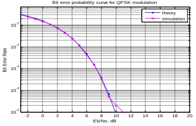
The results in figure 9 and 10 shows the BER v/s SNR for 1 million bits transmitted over AWGN and Rayleigh channel with QPSK modulation. The results are nearly in the same agreement as in the case with BPSK modulation but BER with QPSK modulation introduced more errors due to its symbol containing two bits.

Figure 9: One transmitter and one receiver in AWGN channel with QPSK modulation

Result 4: BER for QPSK in Rayleigh Channel

Figure 10: One transmitter and one receiver in Rayleigh channel with QPSK modulation

-2 0 2 4 6 8 10

10-5 10-4 10-3 10-2 10-1 100

Eb/No, dB

B

it

E

rr

o

ro

r

R

a

te

Bit Erroror probability curve for BPSK modulation

theory simulation

0 5 10 15 20 25 30 35

10-5 10-4 10-3 10-2 10-1 100

Eb/No, dB

B

it

E

rr

or

R

at

e

BER for BPSK modulation in Rayleigh channel

AWGN-Theory Rayleigh-Theory Rayleigh-Simulation

-2 0 2 4 6 8 10 12 14 16 18 20

10-5 10-4 10-3 10-2 10-1

Eb/No, dB

B

it

E

rr

or

R

at

e

Bit error probability curve for QPSK modulation theory simulation

0 5 10 15 20 25 30 35

10-5 10-4 10-3 10-2 10-1

Eb/No, dB

B

it

E

rr

o

r

R

a

te

International Journal of Emerging Technology and Advanced Engineering

Website: www.ijetae.com (

ISSN 2250-2459

, Volume 2, Issue 9, September 2012)

164

Result 5: BER for QPSK modulation with Selection Diversity in Rayleigh Channel

Figure 11: Effect of Selection Combining with QPSK

The result of figure 11 shows the BER v/s SNR for 1 million bits transmitted over Rayleigh channel with QPSK modulation for one and two receive antennas. It can be noticed that with two receive antennas, after utilizing a receiver diversity scheme, Selection Diversity, greatly reduces the BER, for the same SNR of operation. 15 dB SNR operation in the two cases introduces a BER of around 10^-2 with one receiver and 10^-3 with two receive antennas which can be seen from figure 11.

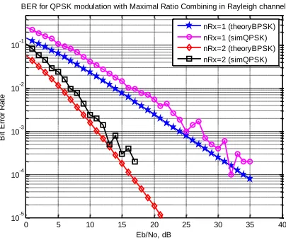
Result 6: BER for QPSK modulation with Maximal Ratio Combining in Rayleigh Channel

The figure 12 shows the simulation results of 1 million bits transmitted over Rayleigh channel with two receive antennas combined together using Maximal Ratio Combining. As we know, MRC is an optimum combiner, it takes better advantage of all the diversity branches in the system therefore, performs better than selection diversity but QPSK is causing slightly greater BER. As compared to selection diversity from figure 11, the MRC offers lower BER say for, 15 dB SNR operation in the two cases introduces BER of around 10^-3 with selection diversity and 10^-4 with MRC with QPSK modulation.

Figure 12: Effect of Maximal Ratio Combining with QPSK

Result 7: BER for BPSK modulation with Alamouti STBC (Rayleigh channel)

The figure 13 represents transmit diversity with two transmit antennas and one receive antenna. We can observe that the BER performance of 2 Tx, 1 Rx Alamouti STBC case has a roughly 3 dB poorer performance than 1 Tx, 2 Rx MRC case.

Figure 13: Alamouti Scheme (2 Transmitters and 1 Receiver)

0 5 10 15 20 25 30 35 40

10-5 10-4 10-3 10-2 10-1

Eb/No, dB

B

it

E

rr

o

r

R

a

te

BER for QPSK modulation with Selection diveristy in Rayleigh channel

nRx=1 (theory) nRx=1 (sim) nRx=2 (theory) nRx=2 (sim)

0 5 10 15 20 25 30 35 40

10-5 10-4 10-3 10-2 10-1

Eb/No, dB

B

it

E

rr

o

r

R

a

te

BER for QPSK modulation with Maximal Ratio Combining in Rayleigh channel

nRx=1 (theoryBPSK) nRx=1 (simQPSK) nRx=2 (theoryBPSK) nRx=2 (simQPSK)

0 5 10 15 20 25

10-5 10-4 10-3 10-2 10-1

Eb/No, dB

B

it

E

rr

o

r

R

a

te

BER for BPSK modulation with Alamouti STBC (Rayleigh channel)

International Journal of Emerging Technology and Advanced Engineering

Website: www.ijetae.com (

ISSN 2250-2459

, Volume 2, Issue 9, September 2012)

165

Result 8: BER for BPSK modulation with 2Tx, 2Rx Alamouti STBC (Rayleigh channel)

The figure 14 represents transmit diversity having two transmit antennas with one and two receive antennas. As can be observed with pink and sky blue lines, the transmit diversity has an advantage of 7 dB improvement and around 14 dB improvement compared to one transmitter system for 10^-3 BER. MRC improves BER, but improvement with transmit diversity is far more than MRC as shown in the simulation result figure 14.

Figure 14: Alamouti Scheme (2 Transmitters and 2 Receivers)

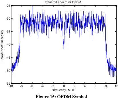
Result 9: OFDM Transmit Waveform

The figure 15 represents an OFDM symbol when a BPSK modulated symbol is transmitted on the 52 used sub carriers according to IEEE 802.11a specifications.

Figure 15: OFDM Symbol

Result 10: BER for BPSK using OFDM

The figure 16 represents BER using OFDM in an AWGN channel.

We can observe that simulated BER results are in good agreement with the theoretical BER for BPSK modulation in AWGN channel which can be seen from figure 7. Therefore, BPSK in AWGN channel and BPSK over OFDM in AWGN channel are same. Say, for achieving BER = 10^-3, 7 dB SNR is required for both the cases mentioned above.

Figure 16: BER using OFDM with BPSK modulation for AWGN channel

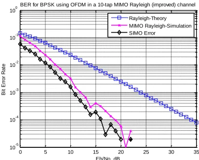
Result 11: BER for BPSK using OFDM in a 10-tap Rayleigh channel

The figure 17 represents BER using OFDM in a 10-tap Rayleigh channel. The simulated BER results are in good agreement with the theoretical BER results. Here, number of Rayleigh paths is equal to 10 tap channels with average channel gain equal to unity. Since, there is no BER improvement in Rayleigh channel; we have simulated it just to observe that BER does not degrade with OFDM. OFDM performance with multipath is comparable to flat fading Rayleigh channel performance shown in figure 8.

Figure 17: BER using OFDM with BPSK modulation for 10-tap Rayleigh channel

0 5 10 15 20 25

10-5 10-4 10-3 10-2 10-1

Eb/No, dB

B

it

E

rr

o

r

R

a

te

BER for BPSK modulation with 2Tx, 2Rx Alamouti STBC (Rayleigh channel)

theory (nTx=1,nRx=1) theory (nTx=1,nRx=2, MRC) theory (nTx=2, nRx=1, Alamouti) sim (nTx=2, nRx=2, Alamouti)

-10 -8 -6 -4 -2 0 2 4 6 8 10

-55 -50 -45 -40 -35 -30 -25

frequency, MHz

p

o

w

e

r

s

p

e

c

tr

a

l

d

e

n

s

it

y

Transmit spectrum OFDM

0 1 2 3 4 5 6 7 8 9 10

10-5 10-4 10-3 10-2 10-1 100

Eb/No, dB

B

it

E

rr

o

r

R

a

te

Bit error probability curve for BPSK using OFDM

theory simulation

0 5 10 15 20 25 30 35

10-5 10-4 10-3 10-2 10-1 100

Eb/No, dB

B

it

E

rr

o

r

R

a

te

BER for BPSK using OFDM in a 10-tap Rayleigh channel

International Journal of Emerging Technology and Advanced Engineering

Website: www.ijetae.com (

ISSN 2250-2459

, Volume 2, Issue 9, September 2012)

166

Result 12: BER for BPSK with 2x2 MIMO and ZF equalizer (Rayleigh channel)

The figure 18 shows BER for BPSK with 2x2 MIMO channel with Zero Forcing (ZF) equalizer. As expected, the simulated results with a 2×2 MIMO system using BPSK modulation in Rayleigh channel is showing matching results as obtained in for a 1×1 system for BPSK modulation in Rayleigh channel can be seen in figure 8. The zero forcing equalizer helps us to achieve the data rate gain, but does not take advantage of diversity gain (as we have two receive antennas).

Figure 18: BER for BPSK with 2x2 MIMO channel using Zero Forcing (ZF) equalizer

Result 13: BER for BPSK using OFDM in a 10-tap MIMO Rayleigh channel with PDP

The simulation below in the figure 19 shows the BER change with increasing SNR, for a MIMO system (2 Transmitters and 2 Receivers) with decreasing strength of the same received bit according to Power Delay Profile (PDP), with frequency selective fading using OFDM, with 64 point FFT with 12 points left for inter service guard.

Figure 19: BER Time Variant Frequency Selective MIMO channel with PDP

Result 14: BER for BPSK using OFDM in a 10- tap MIMO Rayleigh (improved) channel with PDP

The figure 20 shows the final simulation result which is a time variant frequency selective MIMO OFDM (improved) channel. We have incorporated MRC, Alamouti STBC and ZF equalizer which give us better performance as compared with result in figure 19. Say, to achieve BER = 10^-3, we just need to increase SNR to 13 dB whereas, with simple MIMO channel, we require to increase SNR to about 26 dB to achieve the same BER. Hence, we have a MIMO- OFDM model which will obtain higher SNR with comparatively less errors.

Figure 20: BER Time Variant Frequency Selective MIMO OFDM (improved) channel with PDP

0 5 10 15 20 25

10-5 10-4 10-3 10-2 10-1

Average Eb/No,dB

B

it

E

rr

o

r

R

a

te

BER for BPSK modulation with 2x2 MIMO and ZF equalizer (Rayleigh channel)

theory (nTx=1,nRx=1) theory (nTx=1,nRx=2, MRC) sim (nTx=2, nRx=2, ZF)

0 5 10 15 20 25 30 35

10-5 10-4 10-3 10-2 10-1 100

Eb/No, dB

B

it

E

rr

o

r

R

a

te

BER for BPSK using OFDM in a 10-tap MIMO Rayleigh channel

Rayleigh-Theory MIMO Rayleigh-Simulation SIMO Error

0 5 10 15 20 25 30 35

10-5 10-4 10-3 10-2 10-1 100

Eb/No, dB

B

it

E

rr

o

r

R

a

te

BER for BPSK using OFDM in a 10-tap MIMO Rayleigh (improved) channel

International Journal of Emerging Technology and Advanced Engineering

Website: www.ijetae.com (

ISSN 2250-2459

, Volume 2, Issue 9, September 2012)

167

IV. CONCLUSION

The AWGN channel introduces noise which is entirely Gaussian with zero mean and is identical and independently distributed. The noise being additive is uncontrollable but distorts bits only less significantly. Hence, this causes less error. By improving the design of transmitter and receiver, this can be made controllable. The Rayleigh channel which causes fading, causes more bits to go in error, but can be controlled if a perfect knowledge is acquired at the receiver and further at the transmitter. Imperfect channel knowledge is the reason for higher bit error rates in wireless systems, requiring higher SNR‘s to achieve same BER as in the simulation result figures 7, 8, 9 and 10.

After introducing the concept of antenna combining at the receiver, an improvement of about 10 dB is observed. This can be seen from figures 11 and 12. In case of transmit diversity, i.e., Alamouti‘s scheme, there is no requirement of channel knowledge at the transmitter. As the number of transmit antennas is doubled, the data is doubled. If we lose out on data rate, the SNR requirement is drastically improved as seen in simulation result figure 14.

In OFDM case, though Rayleigh channel has multipath taps, for each sub carrier, the channel is effectively a single tap channel. Hence, frequency selective fading channel becomes a flat fading channel with OFDM. OFDM performance with multipath is comparable to flat fading Rayleigh channel performance is shown in figures 17 and 9. The time variant frequency selective channel has multiple scopes for error introduction, bit interference, etc. If the channel improvisation concept is introduced, it leads to very high SNR requirement for satisfactory operation. This can be seen from figures 19 and 20 with the MIMO improved channel.

V. FUTURE ENHANCEMENT

This work can be enhanced for 4x4, 8x8, and so on MIMO channels. When the channel is considered to be too much noisy, the Zero Forcing (ZF) equalizer can be replaced with other equalizers like decision feedback or adaptive blind equalizers which will further improve the overall BER performance and hence obtain good results. We can use different modulation schemes like GMSK, OQPSK etc. and can obtain different BER curves. The simulation work can be done on different types of fading channels such as Rician, Nakagami, Weibull channels, etc. More enhanced MIMO encoders can be used for obtaining a much higher capacity MIMO-OFDM channel model.

REFERENCES

[1 ] A. Omri and R. Bouallegue, ―New Transmission Scheme for MIMO- OFDM System‖, International Journal of Next-Generation Networks (IJNGN) Vol.3, No.1, March 2011.

[2 ] Zhongshan Wu, ―MIMO OFDM Communication Systems: Channel Estimation and Wireless Location‖, A Dissertation Submitted to the Graduate Faculty of the Louisiana State University and Agricultural and Mechanical College, May 2006.

[3 ] Chetan N. Chitnis, ―Differential Space Time Modulation and Demodulation for Time Varying Multiple Input Multiple Output Channels‖, A Thesis submitted to the Graduate Faculty of the Louisiana State University and Agricultural and Mechanical College, May 2007.

[4 ] Kai Dietze, ―Analysis of a Two-Branch Maximal Ratio and Selection Diversity System with Unequal Branch Powers and Correlated Inputs for a Rayleigh Fading Channel‖, Thesis submitted to the Faculty of the Virginia Polytechnic Institute and State University, March 30, 2001, Blacksburg, Virginia.

[5 ] Christian Stimming and Gießen, ―Multiple Antenna Concepts in OFDM Transmission Systems‖, 12th _{June 2009.}

[6 ] Shahab Sanayei and Aria Nosratinia, ―Antenna Selection in MIMO Systems, Adaptive Antennas and MIMO Systems for Wireless Communications‖, University of Texas at Dallas, IEEE Communications Magazine, October 2004.

[7 ] Datacomm Research Company, ―Using MIMO-OFDM Technology to boost Wireless LAN Performance Today‖, White Paper Version 1.0, June 1, 2005.

[8 ] Biljana Badic, ―Space Time Block Coding for Multiple Antenna Systems‖, a Dissertation submitted to University of Wien, November 2005.

[9 ] Nagarajan Sathish Kumar K. R. Shankar Kumar, ―Bit Error Rate Performance Analysis of ZF, ML and MMSE Equalizers for MIMO Wireless Communication Receiver‖, European Journal of Scientific Research, ISSN 1450-216X Vol.59 No.4 (2011), pp. 522-532. [10 ]Agilent Technologies, ―MIMO Channel Modeling and Emulation

Test Challenges‖, Printed in USA, January 22, 2010.

[11 ]Farrukh Rashid and Athanassios Manikas, ―Diversity Reception for OFDM Systems using Antenna Arrays‖, Communications and Signal Processing Research Group, Department of Electrical and Electronic Engineering, Imperial College London, IEEE 2006. [12 ]Andreas F. Molisch and Moe Z. Win, ―MIMO Systems with

Antenna Selection‖, IEEE Microwave Magazine, March 2004. [13 ]R Bhagya and Dr. A G Ananth, ―Study of Transmission

Characteristics of 2X2 MIMO System for different Digital Modulation using OFDM and STBC Multiplexing Techniques and ZF Equalizer receiver‖, Department of Telecommunication Eng., RVCE, India, IJCSET June 2011,Vol. 1, Issue 5,210-213.

[14 ]Notes by Prof. Raviraj Adve, ―Receive diversity‖,2003