ScholarWorks @ Georgia State University
ScholarWorks @ Georgia State University
Physics and Astronomy Theses Department of Physics and Astronomy
Fall 2009
Duty Cycle Maintenance in an Artificial Neuron
Duty Cycle Maintenance in an Artificial Neuron
William Halbert Barnett
Georgia State University
Follow this and additional works at: https://scholarworks.gsu.edu/phy_astr_theses
Part of the Astrophysics and Astronomy Commons, and the Physics Commons
Recommended Citation Recommended Citation
Barnett, William Halbert, "Duty Cycle Maintenance in an Artificial Neuron." Thesis, Georgia State University, 2009.
https://scholarworks.gsu.edu/phy_astr_theses/7
This Thesis is brought to you for free and open access by the Department of Physics and Astronomy at
ScholarWorks @ Georgia State University. It has been accepted for inclusion in Physics and Astronomy Theses by an authorized administrator of ScholarWorks @ Georgia State University. For more information, please contact
by
WILLIAM HALBERT BARNETT
Under the Direction of Dr. Gennady S. Cymbalyuk
ABSTRACT
Neuroprosthetics is at the intersection of neuroscience, biomedical engineering, and
physics. A biocompatible neuroprosthesis contains artificial neurons exhibiting
biophysically plausible dynamics. Hybrid systems analysis could be used to prototype such
artificial neurons. Biohybrid systems are composed of artificial and living neurons coupled
via real-time computing and dynamic clamp. Model neurons must be thoroughly tested
before coupled with a living cell. We use bifurcation theory to identify hazardous regimes
of activity that may compromise biocompatibility and to identify control strategies for
regimes of activity desirable for functional behavior. We construct real-time artificial
neurons for the analysis of hybrid systems and demonstrate a mechanism through which
an artificial neuron could maintain duty cycle independent of variations in period.
by
WILLIAM HALBERT BARNETT
A Thesis Submitted in Partial Fulfillment of the Requirements for the Degree of
Master of Science
in the College of Arts and Sciences
Georgia State University
Copyright by William Halbert Barnett
by
WILLIAM HALBERT BARNETT
Committee Chair: Gennady Cymbalyuk
Committee: Vadym Apalkov
Mukesh Dhamala
Andrey Shilnikov
Electronic Version Approved:
Office of Graduate Studies
College of Arts and Sciences
DEDICATION
ACKNOWLEDGEMENTS
I would like to thank Martin Anquez and Dr. Gennady Cymbalyuk.
I am grateful for support from NSF grant PHY-0750456 to GC, and I here show my
appreciation for an equipment grant (Spring 2009) and two travel awards (Spring 2008
TABLE OF CONTENTS
ACKNOWLEDGEMENTS v
LIST OF FIGURES viii
CHAPTERS
1 INTRODUCTION 1
Model Leech Heart Interneuron Synapse 3
Hybrid Systems Analysis 4
Prototype Reduced Heart Interneuron 7
2 APPLICATION OF TECHNOLOGY FOR HYBRID SYSTEMS 9
dSpace Boards 10
Introduction to Programming in Simulink 11
Library for Dynamic Clamp 14
Building Neuronal Models with Simulink for Real-Time 22
Propensity to Hazardous Dynamics 27
4 PHARMACOLOGICALLY REDUCED LEECH HEART INTERNEURON 30
Motivation 30
Roles of IK2 and Ih 32
5 MAINTENANCE OF DUTY CYCLE 37
Saddle-node Bifurcation 37
Control of Bursting Through Coregulation of Slow Currents 38
Maintenance of Duty Cycle 41
6 DISCUSSION 46
PUBLICATIONS 53
LIST OF FIGURES
Figure 1: Basic blocks 13
Figure 2: Elemental functions 17
Figure 3: Higher level equations 19
Figure 4: Neuronal model 21
Figure 5: Rate functions 24
Figure 6: Derivative equations 25
Figure 7: Hodgkin-Huxley model. 26
Figure 8: Switching 28
Figure 9: Examples of activity and temporal characteristics while varying θK2 33
Figure 10: Sample trajectory 35
Figure 11: Examples of activity and temporal characteristics while varying θh 36
Figure 12: Interburst Interval plotted againstθh 39
Figure 13: Bifurcation diagram 41
Figure 14: Linear relationship 43
Figure 15: Congruent lines 44
1. INTRODUCTION
Dysfunction in the operation of the nervous system can elicit behavioral disorder
and disability that disrupts mobility and livelihood. Neuroprosthetics is a new, frontier
discipline at the intersection of neuroscience and biomedical engineering which has proven
itself efficient in returning hearing, sight, and mobility to people challenged by disabilities.
In order to achieve a biocompatible neuroprosthesis, the artificial neurons must exhibit
biophysically plausible dynamics. Hybrid systems analysis could be used to prototype such
artificial neurons. Biohybrid systems are composed of artificial and living neurons coupled
via real-time computing and dynamic clamp. Model neurons must be thoroughly tested
before coupled with a living cell. We use bifurcation theory to identify hazardous regimes
of activity that may compromise biocompatibility and to identify control strategies for
regimes of activity desirable for functional behavior. We construct real-time artificial
neurons for the analysis of hybrid systems and demonstrate a mechanism through which
an artificial neuron could maintain duty cycle independent of variations in period.
One of its key goals is the design of neuroprostheses: implantable artificial devices
restoring the functional dynamics of the corrupted neuronal circuit. There is a strong
demand for a variety of tools for design and prototyping so that neuroprostheses can be
manufactured at the industrial scale necessary for practical medical applications. They will
be developed using the modern technology of computer-brain interface based on real time
systems, e.g. dynamic clamp and hybrid systems analysis.
Hybrid systems combine the parameter controllability of mathematical modeling
with the physical realism of electrophysiological experiments. This approach allows
development. As such, the implementation of hybrid systems is facilitated by developments
in dynamic clamp and real-time computing. These hybrid systems require software
operating in real time on a timescale fast compared to the time constants of ionic currents
involved. Designated real time controllers are necessary to fulfill these real time
requirements. A real time controller is a computer that performs computational tasks on a
strict schedule. Using such a system to control a dynamic clamp enables real time
interaction between simulated and biological cells. Dynamic clamp has been used to
implement artificial ionic currents in and synapses between living cells (Sharp et al., 1993;
Dorval et al., 2001; Butera et al., 2001; Pinto et al., 2001). In hybrid systems, dynamic clamp
provides the interface between the simulated and living neurons (Manor & Nadim, 2001).
The prototyping of a control system proceeds in several stages. First, we design a
mathematical model which incorporates everything we know about the dynamics of the
functional unit, the neuronal sub-circuit, or the neuron. Then we investigate the dynamics
of the model. Different regimes of activity span a high dimensional parameter space in a
typical Hodgkin-Huxley style neuronal model. We establish a subset of this space for which
the resultant model activities share important traits with activity observed in the healthy
neuronal system. Among the important characteristics are spike frequency, burst
frequency, burst duration, coexistence of oscillations and silence, and other properties of
excitability. Detailed analysis of these parameters’ space allows a researcher to select
optimal parameter values for the task at hand. This process is repeated for the intended
synaptic target of the artificial neuron. Next we can create a hybrid system and test the
hybrid have been studied and classified, a new generation of the prototype is to be
designed and tested.
Hybrid systems analysis is a powerful technique that has proven itself in
neuroscience. It is useful as a prototyping tool for biomedical engineers. Previously, the
technology has been used to identify the role of individual currents in specific cellular
mechanisms(Sorensen et al., 2004; Olypher et al., 2006). The intent of prototyping may be
to establish a certain stable regime of circuit activity, but it is hybrid systems analysis that
we use to reveal the effect of explicitly defined ionic currents of the artificial cell on the
activity of a neural circuit. By replacing a component of a living circuit with a
computational cell, we may gain knowledge of its role in the circuit by manipulating
parameters of artificial ionic currents. With prototyping, we seek to take the knowledge of
the role of individual ionic currents and move an unhealthy circuit from a pathological
regime to a healthy regime. We present a set of experiments performed on the leech heart
interneuron as an example of prototyping and hybrid systems analysis. The first study
utilizes a VLSI silicon artificial neuron in which Ih is tuned to examine its interaction with
the synaptic current (Sorensen et al., 2004). The second study uses computational neurons
built with the library we present in 8.2.3 to tune the slow Ca2+ current to show its role in
supporting bursting activity (Olypher et al., 2006).
Model Leech Heart Interneuron Synapse
The canonical model of the leech heart interneuron is composed of eight voltage
gated currents and a leak current (Hill et al., 2001). The eight voltage gated currents are
composed of thirteen gating variables. The mathematical model is composed of fourteen
hybrid system contains a synapse from the artificial cell onto the living cell and a synapse
from the living cell onto the artificial cell. The synaptic current has a spike-mediated
component and a slower modulating component, so the system requires an additional six
differential equations:
,
; .
The membrane potential of the living cell is recorded and passed into the model
system where it is used to evaluate the synaptic current onto the artificial cell. The
membrane potential of the artificial cell is used to evaluate the synaptic current onto the
living cell, which is passed out of the system to be injected by an amplifier into the live cell.
We are able integrate each of these operations with Euler’s method for numerical
integration at 10 to 20 kHz on the DS1103 PPC board. At these frequencies, the artificial
system performs sufficiently fast to produce biophysically plausible trajectories.
Hybrid Systems Analysis
Observations with sharp intracellular electrodes have shown that the HNs spike
tonically when pharmacologically isolated from the cholinergic synapse with bicuculline
methiodide (Schmidt & Calabrese, 1992). However, recordings with extracellular
electrodes under the same pharmacological conditions show that HNs burst endogenously
introduced by piercing the cell with a sharp electrode, is responsible for the onset of tonic
spiking. In order to implement a hybrid system, a sharp electrode is used to inject an
artificial current into the living cell. Even though the HN is an endogenously bursting cell,
dynamic clamp experiments are performed while the cell is in a tonic spiking mode.
Nevertheless, a mutually inhibitory artificial synapse by and onto a bursting model cell is
sufficient to reinitiate antiphase bursting in the living HN (Sorensen et al., 2004; Olypher et
al., 2006). We tune the hybrid system by manipulating parameters of the artificial cell to
identify the mechanisms supporting the half center oscillator.
In order to establish a biophysically plausible hybrid half center oscillator, a certain
amount of tuning is necessary. Key parameters for temporal regulation can be identified in
an analysis of the parameter space ahead of time (Hill et al., 2001; Cymbalyuk et al., 2002),
such that the artificial cell can be adapted to its intended synaptic target quickly at run
time. The uncoupled artificial cell must exhibit slow oscillations of roughly the same
duration as its living synaptic target; Olypher et al., (2006) adapted the leak current to this
end. In order to appropriately model the activation of the synaptic current, the temporal
characteristics of individual action potentials must be conserved between the model and
the living cell. Due to VLSI transistor mismatch, Sorensen et al., (2004) were forced to
adjust spiking characteristics by changing parameters of fast variables.
The heartbeat of the leech is controlled by a central pattern generator (CPG). The
kernel of this CPG consists of pairs of bursting HN cells, which form half center oscillators.
Each HN cell possesses an inhibitory and spike-mediated cholinergic synaptic current
(Schmidt & Calabrese, 1992). As one cell bursts, the synaptic current onto the second cell
prolonged hyperpolarization during the interburst interval activates Ih and removes the
inactivation of ICaS, the slow Ca2+ current (Hill et al., 2001). In this way, ISyn and Ih on the
inhibited neuron control the interburst interval of that neuron (Sorensen et al., 2004). ISyn
causes the hyperpolarization of quiescence and Ih produces the rebound to a depolarized
state. Upon depolarization, the conductance of ICaS becomes very large and slowly dwindles
as the current is inactivated (Olypher et al., 2006). This long lasting inward current
supports the plateau depolarization of the burst and regulates the spike frequency.
The experiments that ascertain the role of Ih and ICaS encapsulate the core essence of
prototyping. Sorensen et al. (2004) show that by decreasing gh in the artificial cell, the
interburst interval of the artificial cell increases. Because the resistance of Ih to synaptic
inhibition has decreased, the artificial cell takes longer to escape the quiescent phase.
Consequently, the burst phase of the HN increases in duration due to the delayed inhibiting
input. When gh is increased in the artificial cell, its resistance to inhibition increases, and
the interburst interval of the artificial cell decreases in duration. Meanwhile, the burst
duration of HN decreases because of the earlier onset of inhibition from the artificial cell.
Olypher et al. (2006) describe the role of ICaS with a similar set of experiments. By
decreasing the time constant of inactivation of ICaS, τh,CaS, the conductance of ICaS falls is
inactivated at a greater rate in response to the depolarization of the burst, so the bursts are
shorter, and the interburst interval of the presynaptic HN is shortened by the reduced
synaptic inhibition. An increase in τh,CaS in the artificial cell allows ICaS to stay active for a
longer period, and the burst duration is greater. The prolonged burst of the artificial cells
leads to a prolonged synaptic current on the HN. The quiescent phase of the HN increases
Prototype Reduced Heart Interneuron
We explore the role of a hyperpolarization activated current and a potassium
current in the periodicity of a Hodgkin-Huxley style neuronal model, by manipulating the
half activation voltage of each. The half activation of K+ currents has been shown to be
regulated by dopamine and serotonin in the pyloric network (Peck et al., 2001). The half
activation of Ih has been modulated by noradrenalin and serotonin in guinea-pigs and cats,
by Ca2+ in ferrets, and by cAMP in ferrets and rats (McCormick & Pape, 1990; Luthi &
McCormick, 1998; Luthi & McCormick, 1999).
Central pattern generators are neuronal networks that control different types of
rhythmic movement. Many of these neuronal circuits maintain phase as the period of
activity changes. Some examples are the network controlling swim behavior in the lamprey
(Wallen & Williams, 1983), the leech heart beat (Wenning et al., 2003; Norris et al., 2006;
Norris et al., 2007), the swim motor pattern in the leech (Friesen & Pearce, 1993), and the
lobster pyloric rhythm (Hooper, 1997). Experimental and theoretical studies show that
phase maintenance may be mediated by synaptic currents (Eisen & Marder, 1984; Nadim et
al., 2003), and modeling evidence suggests that slow gating variables may also support
phase maintenance (Hooper et al., 2009).
In the network controlling the heart beat of the leech, duty cycle is maintained
independent of period as well as phase (Norris et al., 2006; Norris et al., 2007). By studying
the role of these two currents in the maintenance of duty cycle, we show the role of
neuromodulation in maintenance of function critical cell characteristics. We approach the
problem of temporal coordination in central pattern generators by proposing a mechanism
create a prototype artificial neuron with the ability to adapt an aspect of its intrinsic
activity in response to external stimuli.
Our model is a variant on previously published pharmacologically reduced models
of the leech heart interneuron (Cymbalyuk & Calabrese, 2001; Shilnikov & Cymbalyuk,
2005). It is convenient to use this reduced model because the inducing pharmacological
scenario (described below) allows the HN cell to continue to burst after being pierced with
a sharp electrode. In this way, each of our modeling results could be verified
experimentally by implementation of a hybrid system with dynamic clamp in a manner
similar to Sorensen et al. (2004) and Olypher. et al. (2006).
In this manuscript, we describe an easy to learn and use technique with which to
perform hybrid systems analysis. We include a library of functions that are sufficient to
implement a typical dynamic clamp and to construct any Hodgkin-Huxley style model of a
neuron. Then, we provide an example of a real-time implementation of the Hodgkin Huxley
model of the squid giant axon. By manipulating the voltage dependency of activation in
each of the slow currents in the reduced HN, we show the role of each in bursting activity.
We describe general trends in periodicity as these parameters are varied. We identify
2. APPLICATION OF TECHNOLOGY FOR HYBRID SYSTEMS
The automotive, aerospace, and robotics industries rely on extensive prototyping of
the control systems by using technologies of the real-time systems. The same technologies
can be used for the development and testing of the neuroprostheses by using hybrid
systems analysis. A number of dynamic clamp solutions exist that satisfy the requirements
for real-time computation. Real-Time Linux Dynamic Clamp (Dorval et al., 2001) and now
Real-Time eXperiment Interface (RTXI;
the real-time kernel extension for the Linux operating system. National Instruments
(Austin, TX) produces several lines of real-time PXI data acquisition boards in addition to
the LabVIEW software suite which has been utilized for dynamic clamp (Kullmann et al.,
2004). Milescu et al. (2008) have created a dynamic clamp extension for the QuB program
Hybrid systems need well defined control systems and a robust platform in order to
operate effectively in real-time. Our models are built in Matlab & Simulink which is a
programming environment for technical computing (The MathWorks, Inc., Natick, MA).
Simulink has a graphically represented language with extensive libraries of functions for
common mathematical and analytical tasks. Certain of these libraries, such as Real-Time
Workshop, are dedicated to real-time and hardware targeted computing. We use dSPACE
real-time boards: the DS1104 R&D and the DS1103 PPC. dSPACE, Inc. (Paderborn,
Germany) produces and distributes a series of control system oriented real-time boards. A
software package is bundled together with the dSPACE boards. It includes Real-Time
Interface (RTI) and ControlDesk. RTI automatically utilizes block diagrams developed in
graphical user interface with elaborate instrument panels that can be connected with
corresponding model variables for interactive control of real-time application. dSPACE also
provides a number of Simulink libraries for the design of control systems intended
specifically for dSPACE hardware.
Our Simulink library is easy to use. Matlab & Simulink and the dSPACE hardware are
over-the-counter and compatible with modern desktop computers. Additionally, LabVIEW
provides a number of toolkits that allow Simulink models to be configured onto a number
of National Instruments hardware targets. Our readymade templates for Hodgkin-Huxley
type model components can be configured for a specific biological system and directly
executed in real-time.
dSpace Boards
The dSpace DS1104 R&D and DS1103 PPC controller boards are extensively used in
the automotive, aeronautical, and robotics industries to prototype control systems. These
controllers can be installed in most modern desktop computers. The DS 1104 runs a Power
PC 603e microprocessor at 250 MHz with 32 MB of SDRAM and 8 MB of flash memory. A
100-pin serial input/ output ribbon connects the board to the CP1104 data acquisition
board. The CP1104 has 16 BNC ports. The input voltage range is ±10 V on eight analogue to
digital conversion BNC ports. The first four ports are multiplexed over one channel with 16
bits of resolution. Each of the four remaining ports has a dedicated channel with 12 bits of
resolution. The eight output ports each have a range of ±10 V with 16 bits of resolution.
Each has a dedicated digital to analogue conversion channel.
The DS1103 is a full sized ISA card. Alternatively, it can be housed in an external box
750GX microprocessor running at 1 GHz with 32 MB local and 96 MB global SDRAM. Data
acquisition is performed on the CP 1103 board which links to the DS1103 via 3 parallel 100
pin serial ribbons. Thirty-two BNC ports are available over the range of ±10 V with 16 bits
of resolution. Sixteen of the ports are analogue to digital input ports multiplexed over 4
channels. The eight digital to analogue output ports each has a dedicated channel.
While the dSpace boards are primarily used to design and test airplane and car
control systems, they are efficient controllers for prototyping hybrid systems. Hardware
specifications allow a board to simulate model neurons with the speed and fidelity
necessary for electrophysiological protocols. When paired with standard laboratory
equipment such as the AxoClamp-2B (Axon Instruments, CA), a Simulink model can
efficiently run dynamic clamp in real time on the DS1104 or DS1103.
Introduction to Programming in Simulink
Our dynamic clamp is implemented as a Simulink block diagram. We provide a
library of functions which can be used to tailor it to specific needs. We have included a
model of an oscillatory leech heart interneuron as well as basic functions for the
construction of Hodgkin-Huxley type neuronal models and functions to implement all
standard dynamic clamp features.
Simulink is a graphical programming language for designing control systems in the
MatLab programming environment. Operations and functions are represented by
individual blocks or groups of blocks, and the flow of the program is made explicit by
arrowed lines connecting each block. Blocks have input ports, where arguments and
parameters are passed into the block, and output ports where the block returns the results
clicking on a block allows the user to access its properties and options, embedded code, or
the embedded subsystem of blocks. Simulink comes with 15 basic libraries of blocks in
addition to several specialized libraries. The basic libraries contain blocks for math
functions and signal processing, while the specialized libraries are targeted for more
specific applications such as real-time control.
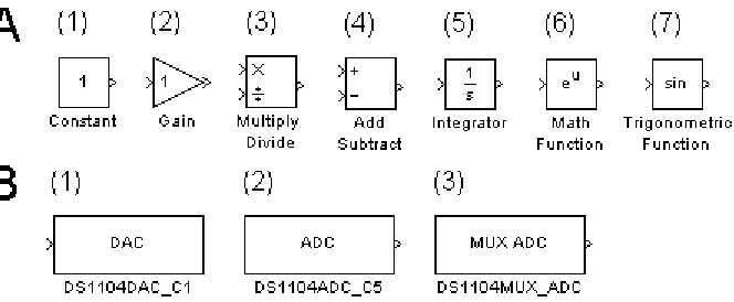
A small set of basic blocks is sufficient to create a neuronal model based on the
Hodgkin-Huxley formalism (Figure1A). Each of these blocks has a number of modes and
functions that can be changed by the developer. The number of input ports and output
ports depends on the block configuration. The Constant block supplies an unchanging
signal of amplitude specified by the user. The Gain block multiplies its input signal by a
factor specified by the user. This can be used in place of the Multiplication/ Division block.
The Multiplication/ Division block is versatile; the number and type of inputs can be
tailored to the task at hand. It accepts scalar, vector, or matrix input. It is also possible to
specify element-wise or matrix operations. Setting this block with a single port that
performs division is equivalent to obtaining the reciprocal for scalar inputs and performing
matrix inversion on matrix inputs. Similarly, the Add/ Subtract block has variable input
ports and acts on both scalar and vector inputs. The Integration block performs numerical
integration. There both fixed step and variable step solvers available to the developer. The
initial conditions for integration can be defined as a parameter internal to the box, or it can
be passed in as an argument. The Math Function block can be set to compute exponents,
Figure 1. Basic blocks. In Simulink, programs are represented as diagrams built out of elemental blocks. Each block represents an individual operation. (A) A small number of blocks representing basic mathematical functions are sufficient to create Hodgkin-Huxley style neuronal models. (B) dSpace blocks provide Simulink models with a means to interact with real world systems. (B 1,2) Channels with dedicated BNC ports can be accessed with individual blocks. The number at the end of the block name corresponds to the channel number of the port on the CP1104 board. (B3) The 16 bit analogue to digital conversion channels are multiplexed. Internal block setting allow the developer to specify to which ports the block is connected.
square roots, powers defined by input, complex conjugation, reciprocals, hypotenuses,
remainders, modulus, transposes and complex conjugate transposes. The Trigonometric
Function block can perform functions including sine, cosine, tangent, arcsine, arccosine,
arctangent, hyperbolic sine, hyperbolic cosine, hyperbolic tangent, and hyperbolic
arctangent.
These Simulink blocks are sufficient to create sophisticated neuronal models, but do
not provide us with a tool to interact with external systems. In order for a model to be
useful for hybrid systems, a control signal from the system must be passed to an amplifier
and into a cell as current, and the amplifier must feed the membrane potential of the cell
back to the model. We move the simulation of the system off of the desktop computer and
onto a peripheral dSPACE board specialized for control systems. dSPACE has provided a set
By passing the desired control signal from a model into a dSPACE block, the signal is routed
out through the data acquisition board to the amplifier. Similarly, a dSPACE block acts as a
source in a Simulink block diagram by routing the membrane potential of the cell back onto
the control board. Blocks compatible with the DS1104 board are located in the DS1104
MASTER PPC library which is located in the dSPACE RTI1104 PPC directory in the Simulink
library browser. dSPACE blocks allow the control system to interact with other devices via
specific ports on the CP1104 (Figure 1B). The DS1104ADC_C5 block reads input from the
board with 12-bit resolution. The C5 suffix indicates that the block corresponds to port five,
but the block is applicable for ADC ports five through eight. The DS1104DAC_C1 block
writes to the digital to analogue port on with 16-bit resolution and is applicable for all eight
digital to analogue ports. For the DS1104DAC and DS1104ADC blocks, the user can specify
the channel to which it is associated by changing the number in the suffix to the desired
port number provided that it is within the applicable range. Finally, the DS1104MUX_ADC
block reads from analogue to digital ports one through four at 16-bits. In order to specify
which port or ports, it is necessary to change the settings of the block.
Library for Dynamic Clamp
The dynamic clamp is a tool used to perform electrophysiological experiments by
injecting current of with particular dynamical characteristics into a living cell. In this
manner, an artificial current with the characteristics defined by the researcher can be
introduced in addition to the existing set of ionic currents endogenous to the membrane.
Alternatively, the dynamic clamp can be used to substitute an artificial current with
dynamic clamp as the link between the computational and living aspects of the system in
order to realize real time control of the temporal characteristics of neuronal dynamics.
Lets consider the hyperpolarization activated current (Ih) identified and measured
(Angstadt & Calabrese, 1989) in the heart interneuron (HN) of the medicinal leech and then
implemented in the canonical model of HN (Hill et al., 2001). The equations for the current
and its activation are
, (1)
, (2)
,
and
,
such that is the maximal conductance, Eh is the reversal potential, and is the
activation variable. The functions and are the steady state and time constant
of activation. These types of models lend themselves to hierarchical organization. At the
highest level, the model, environmental parameters and dSPACE links the data acquisition
board are assigned. Descending into the model reveals a menagerie of blocks and
subsystems.
A block diagram built to perform a specific task can be condensed into a single block
so that complicated systems can be organized into a set of subsystems. A subsystem is a
block diagram that is represented by a single block. Subsystems make it easy to
conceptualize and organize the flow of operations in a block diagram by establishing a
sequestered to lower hierarchical levels while control parameters can be readily available
for manipulation closer to the root of the model.
At the lowest organizational level, system functions are evaluated. The operations
performed at this level are primarily the calculations of steady state membrane potentials
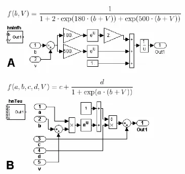
and gating variable time constants. The steady state membrane potential of Ih (1) is a
Boltzmann function (represented by in Figure 2A). The corresponding block
diagram is inserted into the subsystem block hnInfh. The parameter b is an argument of the
function and an input port of the block. It will be assigned by a Constant block at a higher
organizational level. Other parameters of the function, such as the Gain blocks set at 180
and 500, can still be accessed from ControlDesk in real-time, but are left at this lower
organizational level because there is no anticipation of accessing them. The steady state
membrane potential for the activation of Ih is a unique function. The function for the
voltage dependent time constant of activation, however, is used again and again in our
model. From current to current, these functions are represented by the similar equations
differing only in parameter values. Rather than build a dozen unique diagrams for time
constant functions, a small set of equations can be reused to define many gating variables.
A common equation for voltage dependent time constant (2) is also a Boltzmann function
and contained in the subsystem block hnTau (represented by in Figure 2B). In
this case, each of the parameters is assigned at a higher organizational level so that the
same block can be used in more than one gating variable.
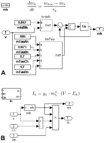
The equation for the derivative of the activation of Ih is (Figure 3A). The
Simulink subsystem block for this equation is mh with one input port, V, for the membrane
Figure 2. Elemental Functions. (A) The function denotes the steady state membrane potential of Ih. The block diagram equivalent to is embedded in the subsystem block hnInfh. In this case, a single parameter is defined at a higher
organizational level. (B) The voltage dependent time constant of activation of Ih can be written as , and its block diagram is embedded in the subsystem block hnTau. This function is not unique to Ih. By defining many parameters at a higher organizational level, this block can be used for different time constants in other subsystems of the same model.
subsystem, the dynamics of the gating variable are defined by the steady state activation
block hnInfh and the time constant block hnTau. At this hierarchical level, the parameters
left undefined inside these blocks are passed in as arguments along with the membrane
potential. It becomes important, when working in ControlDesk, to give these Constant
the specific current, variable, and function with which each is associated so that they may
be differentiated from similar blocks in other subsystems.
Each ionic current is the product of its gating variable subsystems, maximum
conductance, and driving force. Parameters for the maximal conductance and reversal
potential are arguments to be passed into the system. Each ionic current subsystem has
input ports for the membrane potential, the maximal conductance, and the reversal
potential and output ports for the current and each of the intrinsic gating variables (Figure
3B). The neuronal model integrates the negative sum of the ionic currents in order to
produce a value for membrane potential. This membrane potential is then passed into the
ionic current systems to produce values for gating variables, driving forces, and ultimately
a new value for each ionic current. This system itself is condensed into the HN neuron
subsystem (Figure 4).
The mutually inhibitory HNs form a robust half center oscillator. Our model utilizes
a fast spike mediated synapse as the agent of this inhibition (Cymalyuk et al., 2002; Hill et
al., 2001). The activation and modulation of ISyn are dynamical variables dependent on the
presynaptic membrane potential. The driving force of the current, however, is a function of
postsynaptic membrane potential. Spikes on the presynaptic cell lead to an increase in the
conductance of the current, and the membrane potential of the postsynaptic cell
determines how the cell will respond to the new current. The synaptic current on the
postsynaptic cell is summed and integrated along with the intrinsic ionic currents of the
membrane to produce a new value for the membrane potential. This new membrane
potential is fed back into the intrinsic ionic current subsystems but is also passed out of the
Figure 3. Higher Level Equations. (A) The activation variable for Ih is represented by the equation for and can be put together using preexisting functions for steady state of activation and time constant of activation (see Figure 5). At this hierarchical level, constants left undeclared in constituent functions are assigned and passed into the
HNwFastSyn implements the synaptic current by including the ISynS ionic current block
and an additional input port for the presynaptic membrane potential.
A hybrid system has a living component as well as a computational component. An
electrode placed inside of a neuron can read the membrane potential or inject current. Each
of these processes is mediated by an amplifier and a data acquisition board, but these
signals may be ultimately routed to a desktop computer. A procedure running in real-time
allows a researcher to analyze captured data and directly control the dynamics of an
injected current on the fly. By implementing our neuronal model in such a procedure, the
model may interact with a living cell. The membrane potential of the living cell is read of
the electrode and passed to the model running in real-time. This data feed is utilized to
produce a synaptic response on the model neuron, and the response of the model cell is
used to calculate a synaptic current which is then injected back into the living cell. The
subsystem block MathAndLive demonstrates an implementation of just such a procedure
on the DS1104 controller.
By connecting the voltage out and injected current command ports on an amplifier
to the ADC and DAC ports on the CP1104 data acquisition board, the dSPACE ADC and DAC
Simulink blocks provide a neuronal model direct access to its living counterpart. The
membrane potential of the living cell is passed from the ADC block to the model cell where
the live-to-math synapse is calculated. This current is summed with the intrinsic currents
of the model neuron and integrated. Meanwhile, the membrane potential of the model cell
is used to calculate the activation of the math-to-live synapse, and the membrane potential
current is passed into the DAC block, and the signal is fed from the CP1104 board into the
injected current command port on the amplifier.
Building Neuronal Models with Simulink for Real-time Systems
Consider the model of the squid giant axon (Hodgkin & Huxley, 1952). It includes a
fast sodium current (INa), a delayed rectifier potassium current (IK), a leak current (IL), and
an injected current (Iinj). The differential equation for membrane potential takes the form
,
where the gating variables are defined as the differential equations
, , and ,
and the rate functions are
, , ,
, , and ,
such that V is the membrane potential, n is the activation of the potassium current, m is the
activation of the sodium current, and h is the inactivation of the sodium current. The
maximal conductance of an ionic current and its reversal potential are and . The
parameter values used for maximal conductances are = 36 mS/cm2, = 120 mS/cm2,
= 0.3 mS/cm2, and the values used for reversal potentials are = -12 mV, = 115
mV, and = 10.13 mV.
Hodgkin-Huxley style neuronal models typically share a common structure. Gating
variables are defined by voltage dependent rate functions, currents are defined by gating
currents. The equations at each level of a model are often identical apart from numerical
parameter values. Instead of building identical Simulink block diagrams for many functions
in multiple currents, we choose to make block diagrams as generic as possible. If custom
parameter values can be passed into different iterations of a single subsystem block, then
that same block can be used to build more than one gating variable or ionic current. With
this copy-and-paste style of programming, it is easy to compile libraries of multipurpose
functions.
The dynamics of the squid giant axon model are determined by three channel
opening rates and three channel closing rates. The reader will notice that of the six rate
functions, there are only three unique equations. We have defined three functions such that
each of the rate functions can be defined by choosing a function and providing the correct
set of parameters: , , and
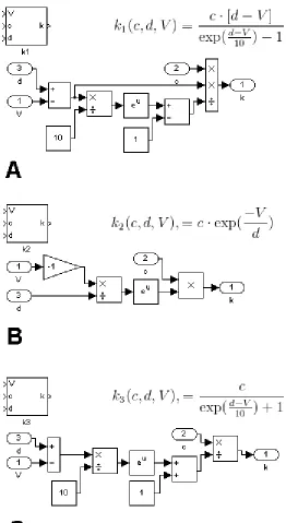
. The functions , , and are embedded in the
subsystem blocks k1 , k2, and k3 with input ports for c, d, and the membrane potential
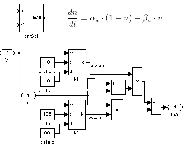
(Figure 5). Block k1 corresponds to rates αnand αm; block k2 corresponds to rates βn, βm,
and αh, and block k3 corresponds to the rate βh.
These rate functions and their associated parameters identify the otherwise generic
gating variable derivative blocks. The gating variable blocks are used in much the same
way; once the correct rate function and parameters are assigned, the derivative block can
be dropped directly into the model. For example, the block dn%dt computes
. At this level of organization, the derivative block calls the rate function
Figure 5. Rate functions. Each of the six rate equations takes the form of one of three equations differing only in parameter values. With just three unique subsystem blocks, all six of the rates can be implemented in Simulink. (A) The block k1 represents function
. This block is used for the rates αnand αm. Block k2 represents function
Figure 6. Derivative equations. The maximal conductance of a current is determined by the component gating variables. The temporal characteristics of each of these gating variables are determined by a pair of rate functions. The rate function blocks are inserted into a generic derivative block, and the parameter inputs are specified. Take, for example, the block. Blocks k1 and k2are the appropriate rate equations for αnand βn, and the rate parameters
current gating variable and membrane potential value to evaluate these functions and
outputs the derivative of the gating variable with respect to time. Ionic current
computation is a parallel process to gating variable computation in this model. The
equations governing the conductances of the ionic currents are largely unique, so there is a
dedicated box for each current.
In this model, integration is performed as a vector operation. The derivatives of each
of the variables of state are multiplexed into a single signal and passed into the integrator.
In the block diagram, the multiplexed signal is a darker connecting arrow (Figure 7). The
many methods for numerical integration. The simplest method is Euler’s algorithm where,
given some initial value of a function , the derivative of the function is evaluated at
discrete intervals of time in order to produce a numerical approximation of as it evolves
over time. Other methods may produce a more accurate approximation but often require
[image:36.612.78.337.210.604.2]that the function’s derivative be evaluated many times for
each iteration of integration. These methods may be undesirable for real-time simulation
because of time constraints on the algorithm.
Propensity to Hazardous Dynamics
For the parameter values provided by Hodgkin and Huxley, this model does not
exhibit membrane potential oscillations. Brief depolarizing injected current pulses may
elicit individual action potentials, and a constant depolarizing injected current may bring
the cell into a regime of tonic firing. Moreover, for Iinj of sufficient amplitude, there exists a
stable stationary state separated from the spiking regime by a stable manifold of a saddle
type orbit (Guttman et al., 1980). Additional pulses of current may push the trajectory of
oscillations beyond this orbit such that the membrane potential converges to the stable
stationary state (Figure 8 A). Conversely, a current pulse of sufficient amplitude may push
the trajectory outside of the basin of attraction of the stationary state, leading to membrane
excitation and tonic spiking (Figure 8 B). This scenario can be tested by applying episodes
of noise to the artificial Hodgkin–Huxley neuron.
First, though, we introduce a mechanism through which a model can interact with
external processes. The dSpace PCI board will host the model, and its data acquisition
channels will be available. Conveniently, the basic Simulink blocks and the dSpace data
acquisition blocks may all be compiled to run in real-time. The DS1104MUXADC block
reads input from the first four analogue to digital channels on the CP1104. This block will
supply the noisy stimulus current used to switch the model from spiking to silence. The
ADC block feeds directly into a gain block, so that the noise signal can be amplified to
sufficient magnitude and is also modified by an offset current to keep the ambient stimulus
After the model is compiled with Real Time Workshop, it is loaded onto the dSpace
board. We provide an example ControlDesk layout, hazardhh.lay, that contains tools to
interact with and control the model in real-time. It includes a plot and control panel to
[image:38.612.88.438.192.559.2]monitor and capture the membrane potential and stimulus current. The layout also
includes two numerical input fields to control the amplitude of the stimulus current and the
offset current. It may be necessary to zero the ambient stimulus current by adjusting the
offset block so that a baseline stimulus current does not modify the dynamics of the cell.
We found our input to be balanced with an amplitude gain of 200 and an offset current at
1.5.
Using a conducting pin or wire, carefully touch the ADC1 port on the CP1104 and
monitor the voltage and current traces in ControlDesk. As long as contact with the port is
maintained, noisy excursions should be observed in the stimulus current. Notice that by
simultaneously touching the electrode and the surrounding shield, a different waveform is
produced. If initial contact with the electrode does not produce switching behavior,
repetitive tapping may be sufficient, or it may be necessary to change the stimulus
4. PHARMACOLOGICALLY REDUCED LEECH HEART INTERNEURON
Motivation
The model {INa, IK2, Ih} is based on a previously published model (Cymbalyuk &
Calabrese, 2001; Shilnikov & Cymbalyuk, 2005). In order to reduce the mathematical
complexity of the system, we simulate the activity of a heart interneuron in bath with Co2+
and 4-aminopyridine (4-AP). Application of Co2+ blocks Ca2+ currents and the synaptic
current. Application of 4-AP blocks most of the K+ currents. The remaining currents in this
model are the leak current (IL), the slow outward potassium current (IK2), the fast sodium
current (INa), and a constant polarizing current. Our model also includes the
hyperpolarization activated current (Ih) which is present in this pharmacological scenario
but has not been previously represented in reduced models. Intracellular recordings in
these conditions show slow seizure-like oscillations with periods that are tens of seconds
long (Opdyke & Calabrese, 1994).
The membrane potential (V) and each of the ionic currents are modeled using
Hodgkin-Huxley formalism. The gating variables are the activation of IK2 (mK2), the
inactivation of INa (hNa), and the activation of Ih (mh). The activation of INa is taken to be
instantaneous. It is modeled as the steady state curve of the activation of the current which
is a function of V. The steady state curves of mK2 and hNa are also sigmoidal functions of V,
and the steady state of mh is a modified sigmoidal curve. The time constants of mK2 and hNa
are constant, and the time constant of mh is a function of V. The half activation value of a
sigmoid function of V is the value of V at which the value of the function is one half. The half
activation parameters for the activation of INa and hNa are not varied. The half activation
,
,
,
,
The slow variables in this system are mK2 and mh with time constants of
approximately one and two seconds. As such, the temporal characteristics of these
variables are instrumental in the dynamics of bursting activity. By systematically
manipulating parameters that determine the dynamics of the slow variables, we can
observe the range of bursting activity and bifurcations between qualitatively distinct
regimes of neuronal activity. Bifurcation theory allows us to make predictions concerning
the temporal characteristics of the dynamics of bursting nearby the critical transitions
associated with the onset of bifurcation.
Bifurcation analysis of the model {INa, IK2, Ih} was performed by shifting the half
activation values of the two slow variables from the canonical values. While systematically
varying these parameters, we observed the periodicity of bursting activity. The period of
bursting activity is the time measured from the first spike of one burst to the first spike of
the next. The burst duration is the time measured from the first spike of a burst to the last
spike of that burst. The interburst interval is the time measured from the last spike of a
burst to the first spike of the next burst, and the duty cycle is the ratio of burst duration to
Roles of IK2 and Ih
We established the role IK2 plays in supporting bursting activity in a model lacking
Ih. Shilnikov and Cymbalyuk (2005) showed that as the half activation parameter
approaches a critical value at the border of bursting and tonic spiking, the burst duration
grows in accordance with a saddle node for periodic orbits while the interburst interval
remains largely unchanged. By shifting the half activation voltage away from the border of
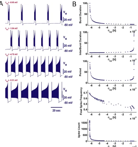
bursting and tonic spiking, we observed a range of bursting that is approximately 0.006 V.
Bursting activity at the lower end of this range consisted of long bursts interrupted by
short interburst intervals, but activity for larger values of θK2 consisted of short bursts with
long quiescent phases (Figure 9A).
Bursting activity transitions to tonic spiking at the border of bursting for lower
values of θK2, and bursting activity transitions to quiescence at the border of bursting for
higher values of θK2. We analyzed the evolution of activity with changes in θK2 by
comparing the temporal characteristics of successive simulations (Figure 9B). Shilnikov
and Cymbalyuk (2005) showed that for values of θK2 where the burst duration was very
sensitive to changes in the control parameter, the interburst interval remained constant.
Similarly, we observed that for values of θK2 where interburst interval of bursting activity
was sensitive to θK2, the burst duration remained constant. Over the entire observed range
of bursting, the spike frequency at the end of the burst fell between 5.4 and 5.7 Hz.
We introduced Ih and studied its role in bursting activity. The initial values we chose
Figure 9. Examples of activity and temporal characteristics while varying θK2. (A) Example
trajectories with burst durations and interburst intervals of approximately 2 seconds
(Figure 10). By varying θh, we observed bursting over a range of 0.06 V. We found that Ih
primarily modulated the interbust interval in this model (Figure 11A). At the border of
bursting for lower θh (-0.004 V) we observed a transition to depolarized silence. At the
border of bursting at θh=0.056 V, bursting transitioned to hyperpolarized silence. As θh
approached the lower border for bursting, the burst duration roughly tripled and became
irregular from burst to burst (Figure 11B). As θh approached the upper border of bursting,
the interburst interval became very large. In both cases, either the burst duration or
interburst interval was sensitive to changes in θh while the other remained roughly
constant. Similar to the previous system, the final spike frequency fell in a narrow range as
Figure 11. Examples of activity and temporal characteristics while varying θh. (A) Example
trajectories over a range of values for θh. (B) Temporal characteristics for trajectories
computed at different parameter values. Trajectories with irregular burst durations can be identified by the large standard deviations. Large jumps in final spike frequency
5. MAINTENANCE OF DUTY CYCLE
We used curve fitting to determine the laws that governed the evolution of temporal
characteristics as bifurcation parameters approach critical values. Once identified, these
laws allowed us to characterize the type of bifurcation the system undergoes at the critical
value. Numerical methods allowed us to characterize the type of and compute parameter
space coordinates for these bifurcations directly. We were able to re-characterize the
control parameter of bifurcation as the distance along a line made up of points in the
parameter space sharing the same duty cycle.
Saddle-node Bifurcation
A saddle-node bifurcation for stationary states occurs when a fixed point is born,
and separates into two fixed points. In the one dimensional case, a semi-stable fixed point
separates into a stable and an unstable fixed point. In the case of two or more dimensions, a
node is born and separates into a saddle and a node. In the case where a
saddle-node bifurcation occurs on an orbit, the orbit dies on the fixed point. It is possible to detect
the approaching bifurcation by observing changes in the period of the orbit. For a given
variable q, the derivative of q with respect to time approaches zero for a certain phase of
the orbit as the bifurcation parameter x approaches a critical point c. As such, the orbit
slows down when it passes near this bottleneck. As x approaches c, the period increases
proportionally to one over the square root of the difference between the critical point and
the control parameter: .
The fold limit cycle is similar to the saddle-node bifurcation for stationary states, but
pertains to the birth of limit cycles. As the bifurcation parameter changes, a saddle periodic
near a fold limit cycle experience a bottle neck in a similar way as trajectories that pass
near a saddle-node for stationary states. Rather than spending more and more time nearby
the stationary state, trajectories spend more and more time oscillating nearby the saddle
periodic orbit. The period of these trajectories grows proportionally to one over the square
root of the control parameter. This has been reported previously for the first example in
the previous chapter (Shilnikov & Cymbalyuk, 2005). We observed a saddle-node
bifurcation for stationary states for both cases presented in the previous chapter. As θK2 is
varied towards the border of bursting and silence and θh is varied towards he border of
bursting and hyperpolarized silence, the interburst interval of each grows in accordance to
the saddle-node bifurcation (Figure 12).
Control of bursting activity through coregulation of slow currents
We observed the behavior of the system by extending our analysis onto the plane of
θhand θK2. The parameter θh was varied from -0.153 V to 0.147 mV, and θK2 was varied
from -0.025 V to 0.010 V. For every value of θhobserved, there was a finite window in θK2
where bursting was possible. For values of θh above 0.010 V and below -0.053 V, changes in
θh ceased to modulate bursting activity. When θh is above 0.057 V, θh drops below the range
of bursting behavior. In other words, Ih activates below the lowest voltage in a burst, and
the current is effectively shifted below the bursting activity. Further increases to θh are
superfluous. Similarly, when θh is below -0.053 V, the curve for steady state of activation is
close to one for the range of membrane potentials expected in a burst. In this case, Ih is
[image:49.612.81.438.60.638.2]
We observed a complicated relationship between the periodicity of bursting
behavior and the half activation parameters θhand θK2. Changes in period over the
parameter space were the result of variations in interburst interval and/or burst
duration. The periodicity was generally characterized by two cases: above and below a line
at roughly 0.057 V in θh. The period generally increased for values of θh approaching this
line from below. Period also grew in this region as θK2 decreased. The union of these two
cases, where θK2 was near the point of burst termination for negative values and θh was
near 0.057 V, showed a very sharp increase in period observed to around 30 s. The region
above the line at 0.057 V shows no change in period with any change in the parameter θh,
and since the activation of Ih was so hyperpolarized, the system was effectively reduced to
three dimensions. Bursting was observed between the fold limit
cycle and saddle-node bifurcations at -0.006 V and 0 V in θK2. As the bifurcation parameter
approached either of these values, the period grew towards infinity.
As θK2 decreased towards burst termination, the peak burst duration observed can
be broken into categories that correspond to three ranges for θh: below -0.053 V, between
-0.053 V and 0.057 V and above 0.057 V. Below -0.053 V in θh, burst duration was wholly on
the order of half a second. In this region below θK2 values of 0.008 V, burst duration was
slightly longer on average but also became irregrular. Above –0.053 V in θh, the border of
bursting behavior for lower values of θK2 dropped to around -0.006 V at the line where θh
was 0.057. Additionally, the burst duration at the border increased as θK2dropped and θh
grew to the point where the border was defined by a fold limit cycle (Figure 13). Nearby
Figure 13. Bifurcation diagram. Points on the map corellate to values of θh and θK2 for which bursting was observed. Warmer colors correspond to higher duty cycle, and cooler colors correspond to smaller duty cycle. Excluded from this rule are the series of green points which have a duty cycle between 0.55 and 0.60. The black dotted line corresponds to a fold limit cycle. The upper black line is a saddle-node bifurcation. The lower black line is an Andronov-Hopf Bifurcation.
monotonically to infinity as θK2approached the fold limit cycle for values of θh above 0.057
V.
Maintenance of Duty Cycle
Further analysis was performed by computing the duty cycle of bursting behavior
(Figure 13). Duty cycle is the ratio of burst duration to period: a neuron that exhibits
observed high duty cycles were bursting terminated at lower values of θK2. Duty cycle did
not vary with θhfor values above 0.057 V. For values of θK2 close to the saddle-node
bifurcation, the duty cycle approaches zero, and for values of θK2 close to the fold limit
cycle, the duty cycle approaches one.
For values of θh below -0.053 V, a similar trend was observed. Greater values for
duty cycle were found at the lower border of bursting in θK2, and lower values for duty
cycle were found at the upper border of bursting in θK2. In neither case were we able to
achieve arbitrarily large or small duty cycles. Between values above -0.053 V in θh, the peak
value for duty cycle followed the border of bursting as θh grew to 0.057. For coordinates in
the parameter space nearby the lower border of bursting in this region, duty cycle
decreased most rapidly for coordinates moving away from the border up to approximate
value of 0.004 mV in θK2. Beyond this point, further changes in duty cycle were primarily
dependent on θK2.
We observed subsets of data points for which duty cycle remained constant despite
smooth growth in the period of bursting (Figure 14). We were able to further characterize
the bifurcation diagram by limiting observation to a small range of duty cycle (green points
in Figure 13). We found an apparently continuous curve of equal duty cycle that was
linearly dependent on θK2and θh in the range between the saturation and removal of the
activation of Ih. Above and below parameter values for which this saturation and removal
occurred, equal duty cycle curves no longer varied with θK2.
Similar and congruent curves existed nearby in the parameter space for different
duty cycles (Figure 15). Each curve is roughly parallel to the border of bursting defined by
Figure 14. Linear relationship. Burst duration and interburst interval maintain a linear relationship with period. Duty cycle does not vary.
bifurcation diagram. These curves increased in period from the bottom of the bifurcation
diagram where the activation of Ih is saturated to the top where Ih is no longer activated.
Just as the period of bursting was no longer dependent on variations in θh above and below
certain parameter values, the period along equal duty cycle curves no longer varied with θh
above and below these values.
As each curve approached the point at which the activation of Ih is fixed at zero, the
period grew proportionally to one over the square root of the distance along a curve of
equal duty cycle (Figure 16). We characterized this distance by computing the distance of
Figure 15. Congruent lines. We show four congruent lines of equal duty cycle. Each set of points was fitted to the form y=mx+b. The circular points correspond to a duty cycle between 0.81 and 0.8 and fitted to m=-12.91 and b=-0.304. The triangular points correspond to duty cycles
between 0.76 and 0.75 and fitted to m=-9.374 and b=-0.217. The square points correspond to duty cycles between 0.71 and 0.7 and fitted to m=-6.854 and b=-0.156. The pentagonal points correspond to duty cycles between 0.66 and 0.65 and fitted to m=-5.274 and b=-0.118.
of bursting in parameter space contracts as Ih is shifted out of the bursting regime, and the
period of bursting increases. The distance in parameter space from both the saddle-node
bifurcation for stationary states, and the fold periodic orbit decreases with this contraction
until Ih is no longer activated. Up to this point, trajectories on a line of equal duty cycle
interburst interval grow proportionally (Figure 14 and 16). Without compensation in Ih, the
period cannot increase while duty cycle is maintained, and the bifurcations become entirely
[image:55.612.79.539.150.525.2]dependent on θK2.
6. DISCUSSION
Our goal was to construct a biophysically plausible and biocompatible artificial
neuron. We satisfied the real-time requirements of hybrid systems with Simulink’s Real
Time Workshop and dSpace hardware. We showed the preservation of a behaviorally
critical characteristic, constant duty cycle, in a neuronal model.
Neuroprosthetic devices will one day routinely treat neurological disorders by
monitoring and regulating the electrical activity in the central nervous system. Such
brain-machine interfaces will need to be small, fast, and power efficient. The introduction of the
analogue very-large-scale integration (aVLSI) neuron provides a framework for artificial
cells and neural networks that satisfy these criteria (Mahowald & Douglas, 1991). Silicon
neurons working in tandem with living networks have produced biologically valid patterns
(Jung et al., 2001; Sorensen et al., 2004). The optimization of circuit design promises
efficient and biocompatible VLSI chips (Rachmuth & Poon, 2008). The clinical distribution
of these neuroprostheses will require industrial manufacturing of implants. Like any other
industry, the neuronal models upon which these devices will be based will need to be
tested before the production process begins. Testing could be done with a hybrid system:
artificial neurons can be interfaced with biological neurons or networks of neurons with a
dynamic clamp. By tuning characteristics of the artificial cell, an analysis of the hybrid
system can reveal pathological or otherwise undesirable neuronal or network states. By
prototyping neuroprostheses in this manner, a researcher can design an artificial cell that
meets implant design parameters without compromising the dynamics of the biological
In order for a hybrid system to function properly, the artificial system must be
simulated on a computer such that computational cell is able to respond to the living cell
without interruption. These computational necessities are often accomplished with
real-time computing in which operations are performed on a strict schedule. While most
modern desktop computers are capable of running real-time software, most modern
operating systems are not real-time. Developers must rely on specialized products to
implement real-time applications: a real-time operating system runs a program directly on
the desktop computer or a program is run on a real-time peripheral device (a control
board) that is controlled from the desktop computer. A prominent supplier of real-time
control boards and support software is dSpace. dSpace products are commonly used for
prototyping control systems in the robotics, automotive, and aerospace industries. dSpace
software automatically utilizes a system designed in Simulink and executes it on a real-time
control board. We realize hybrid systems by designing neuronal models in Simulink and
using dSpace to implement these models in real-time.
Matlab & Simulink provide a high level programming language designed for
technical and high performance computing. Simulink is a graphical programming
environment; Simulink programs look like flow charts. Individual operations are
represented as blocks, and blocks are connected with arrows showing how the output of
one block is used by other blocks. Larger mathematical expressions may be contained by a
single block so that, in our case, biophysical functions such as current, conductance, and
driving force can each be represented as individual blocks. Even an inexperienced user can
Simulink’s drag-and-drop programming style. As in any high level programming language,
program components can be reused to reduce development time.
We provide a library of functions in Simulink sufficient to create a neuronal model.
This library includes individually implemented artificial currents, voltage dependent
steady state curves, and voltage dependent time constants. Moreover, these functions
provide a template with which to construct novel neuronal models. Many of our functions
are standardized so that each numerical parameter is specified by the user. By providing
custom parameters based on experimentally measured ionic currents, a researcher could
implement any number of currents not found in our library. These models are designed to
be used as real-time control systems for a dynamic clamp.
In order for a neuroprosthesis to assume the role of some functional neuronal
circuit, it must behave as though it is a functional neuronal circuit. That means that it must
continue to have a functional role in its host as the local and global neuronal environments
change over time. Factors such as fatigue, age, injury, and drug use can all change the way
neuronal circuits and their synaptic targets function. Prosthetic activity must be robust so
that the larger neuronal circuit remains resistant to degeneration. We use the numerical
and analytical tools of dynamical systems theory to study the mechanisms through which
these environmental factors enact neuromodulation in order to identify manifestations of
pathology in model neurons.
Dynamical systems theory provides a theoretical foundation for sensitivity analysis
in mathematical models. Qualitative aspects of a dynamical system can be revealed through
mathematical analysis of critical parameter values and initial conditions in the context of