DISOCIAL MEDIA SYNCHRONIZATION MODEL: IN ASSOCIATION WITH DEVELOPING SMALL MEDIUM ENTERPRISES SALES INFORMATION SYSTEM

(1)

ISSN: www.jatit.org E-ISSN:

SCALE TO DISEASE PRONENESS (SDP) & SCALE TO

DISEASE INEPTNESS (SDI): DESIGN OF HEURISTIC

METRICS TO ASSESS HEALTH CONDITION TOWARDS

HEART DISEASE PRONENESS

RAMANA NAGAVELLI1 DR.C.V.GURU RAO2

1

Department of Computer Science and Engineering, Kakatiya University, Warangal, India

2

Professor, SR Engineering College, JNTUH, Warangal, India

Email: [email protected] [email protected]

ABSTRACT:

The early stage diagnostics of heart disease is a challenging task. The interdependent and high complexity characteristics and factors related to heart disease combined with human constraints contribute towards the necessity of intelligent medical systems. In this paper we design heuristic metrics for predicting patterns of heart disease, the Scale to Disease Proneness (SDP) metric and Scale to Disease Ineptness (SDI) metric. The prediction system to be efficient in the performance and the scalability requirements has to select an optimal set of attributes from the data for which in our approach we make use of canonical correlation analysis. The test outcomes shown that the heuristic scales SDP and SDI devised here in this paper delivered optimal performance towards predication accuracy, also scalable and robust in the context of computational and process complexity. The approach tends to deploy easily to focus according to individual risk levels of the disease.

Keywords: Health Mining, DDP, SDP, SDI, Disease prediction, Decision Support System, Machine Learning

1. INTRODUCTION

The disease diagnostic decisions dependence on medical Decision Support Systems (DSS) [11] [3] has been augmented by the development of complicated disease-related insights dependent on numerous minute details, fast decision making requirements necessary for most critical cases, meeting the efficient care as well as enhanced value requirements of healthcare consumers, constraints of medical professionals having sufficient time, knowledge to handle each individual cases, the basic human limitations of applying the vast amount of data that may be applicable to any case, and the cost, time factors

associated with training every medical

professional.

The patterns and relationships hidden in huge databases [8] of mobile, internet, and medical

data, extracted with data mining [6] techniques

serve different industry information [7]

requirements. The data mining approach

combines techniques of database, artificial intelligence (AI), machine learning (ML), statistics and other tools [5]. The database is stored, organized, represented, and retrieved with disease diagnosis systems. The huge unordered data is categorized and classified into specific classes with algorithmic techniques of AI, NN, ML etc. The data mining strategies are modeled for different requirements such as, clustering,

classification, pattern discovery, building

predictive models, etc. however classification and prediction are the most primary functionalities widely applied. In classification feature selection techniques based on supervised and unsupervised learning model the data into groups for better

analysis and comprehension. The prediction

(2)

strategy is implied to support decisions in all stages of diagnosis, prognosis and therapy processes.

The data mining strategies are applied with two techniques; supervised learning which uses machine learning algorithms to learn, train and classify the unorganized data with a training set, and unsupervised learning where no training set is used by the algorithms. The data mining techniques such as, bagging algorithm, naïve bayes (NB), and decision tree (DT), neural network (NN), kernel density (KNN), and support vector machine (SVM) both individually and in combination are used in the diagnosis and

prediction process. The strategies are

implemented with medical systems offering diagnostic support, for large volume of disease data, to assess the complex interdependence between various disease related factors, cause effect symptoms, and the true factors leading to the disease. The models of classification are able to classify the data without any hierarchy into specific labels, and the models of prediction show prediction functions of continuous-value [9]. The different data mining methodologies have varying accuracy levels in, processing the data, retrieving relevant information and predicting the disease.

The heart disease [4] diagnostics process is effective and simpler based on an analysis using statistics and data mining approaches. The attributes of heart disease have complex relationships and involve unique challenges in understanding if a patient’s health characteristics imply causality. The modelling of heart disease-related data helps in generating parameters of risk factors enabling early stage diagnosis of high risk patients and timely administration of effective treatment. Several such analyses have studied the reasons of heart diseases and found that heart disease is mostly caused due to, heart attack, stroke or chest pain. The heart related problems which can be treated with the data mining strategies and techniques are, coronary heart

disease (CHD) or heart attack [12],

cerebrovascular disease (CVD) or stroke,

hypertensive heart disease due to elevated blood pressure (hypertension), peripheral artery disease (PAD) due to reduced blood flow because of narrowing of arteries, rheumatic heart disease (RHD) or valve damage due to infections,

coronary heart disease (CHD) or the heart defects that occurs during birth, and heart failure due to the heart muscles unable to pump enough blood to the heart, Inflammatory heart disease due to inflammation of the heart muscles. The database of heart disease obtained from the medical reports involves various elements having high number of attributes and our study for dimensionality reduction, attributes optimization and diagnostic process simplification, proposed the diseased heuristic scales SDP and SDI. The heuristic scale

approach finds applications in financial

forecasting, credit analysis, etc. and our study from the analysis of huge medical record database finds heuristic scales, with optimal attributes and searches for hidden knowledge among the relationships and explores the inadequately evaluated relationships effects.

2. RELATED WORK

A recent study states in the year 2010, considering all the reasons of deaths [2] in the world, the contribution of cardiovascular diseases (CVDs) was greater comparatively. The study also finds by the year 2030 about 76% of the deaths in the world will be due to non-communicable diseases (NCDs) [1] of which cardiovascular related diseases that are on the rise due to, alcohol, consumption, use of tobacco, lack of exercise, diet, etc. [3] would account for third of all the deaths [2]. Medical and health care professionals capability of accurately diagnosing

heart disease is multiplied with the

implementation of strategies, and techniques of data mining such as, classification, clustering, regression, artificial intelligence (AI), neural networks (NN), association rules (AR), decision trees (DT), genetic algorithm (GA), support vector machine (SVM), K-nearest neighbor (KNN) etc.

(3)

Neural Network based on Multi-layer Perceptron (MLP) with back propagation learning algorithm has more efficient performance of disease prediction in comparison to the other algorithms considered. The other approaches tested, K-Nearest Neighbor, a basic Neural Networks

approach, clustering based Naïve Bayes

classification approach, show lower predictive capabilities [14].

However a reduction of the test data and number of class labels shows better performance using, Decision Tree (DT) and a comparable precision

sometimes is obtained with Bayesian

classification. In this test, 909 heart diseases patient records are considered where the dataset is divided into two sets equally, training dataset comprising of 455 records and testing dataset comprising of 454 records. In the learning process 13 regular attributes are used [12] with 2 class labels “Heart Disease” and “No Heart Disease”. The prediction process using the algorithms DT and NBC based on Weighted Associative Classifier (WAC) attains accuracy of 81.51% maximum. The accuracy is improved to 99.2% with DT technique, compared to other techniques when the data size is reduced and the attributes reduced to 6 from 13 with genetic algorithm (GA).

A prediction system for predicting heart attack based on algorithm ID 3, by Hnin Wint Khaing [15] represents various risk levels as a decision tree. In the preprocessing stage, K-means clustering algorithm is used to cluster the heart disease database and mine associated data of heart attack. The further mining of the data with MAFIA (Maximal Frequent Item set Algorithm) yields recurring patterns of heart attack. The algorithm ID3 used as training algorithm depicts with a decision tree the heart attack associated risk levels. The important patterns selected are used to train the ML algorithm for improving the disease prediction efficiency. The tests performed on the system for predicting heart attack show the approach is effective in accurately predicting the risks of occurrence.

A statistical technique Canonical Correlation Analysis (CCA) [21], [22] of earlier times has become widely used in the previous 10 years due to its reasonably worthy data analysis application results providing better understandable insights into the problems. The approach measures the

linear relationships existing amongst any 2,

X

and

Y

multidimensional datasets with

auto-covariance’s and cross-auto-covariance’s matrices of second-order.

The prediction of the risk levels of heart attack has been studied by Chaurasia and Pal in the paper [16]. The study is based on the database obtained from UCI machine learning heart disease repository which comprises of 4 data sets one each from, Cleveland Clinic Foundation of United States, Hungarian Institute of Cardiology, V.A. Medical Center, California and University Hospital, Switzerland. The database is tested with data mining techniques such as, Naïve Bayes, J48 decision tree and Bagging based on 11

significance attributes. The test results

demonstrate, bagging based approach compared to techniques of Naive Bayes and J48, has more precise performance and effective prediction of heart attack.

(4)

ISSN: www.jatit.org E-ISSN: 3. DEFINING A HEURISTIC SCALE TO

DISEASE PRONENESS (SDP) AND SCALE TO DISEASE INEPTNESS (SDI)

3.1 Dataset Preprocessing

The heart disease diagnosed patient record contains 76attributes with values of type continues and categorical. The given dataset [19] is formed with patient records with 14 attributes that are considerable and benchmarked in earlier research [15,16, 17, 18]. Along the side of the

heart disease patient records considered for experiments, we also opted to the patient records that are noticed as normal and not affected by heart disease. In regard to facilitate the optimization process devised here, the values of the attributes in the given dataset should be numeric and categorical. Henceforth, initially we convert all alphanumeric values to numeric values and then the continuous values to be converted to categorical.

Table 1: Description Of Dataset Attributes [20]:

Attribut e ID

Attribute of Complete

Record Description Value state of the Attrib

1 #3 age: patient age (in years)

2 #4 sex: gender (1 = male; 0 = female)

3 #9 cp: chest pain type

(Value 1: typical angina, Value 2: atypical angina, Value 3: non-anginal pain, Value 4: asymptomatic)

4 #10 trestbps: resting blood pressure (in mm Hg on admission to the hospital)

5 #12 chol: serum cholestoral (in mg/dl)

6 #16

fbs: fasting blood sugar > 120

mg/dl (1 = true; 0 = false)

7 #19

restecg: resting

electrocardiographic results

(Value 0: normal, Value 1: having ST-T wave abnormality [T wave inversions and/or ST elevation or depression of > 0.05 mV], Value 2: showing probable or definite left

ventricular hypertrophy by Estes' criteria)

8 #32

thalach: maximum heart rate achieved

9 #38 exang: exercise induced angina (1 = yes; 0 = no)

10 #40

oldpeak: ST depression induced by exercise relative to rest

11 #41

slope: the slope of the peak exercise ST segment

(Value 1: upsloping, Value 2: flat, Value 3: down sloping)

12 #44

ca: number of major vessels (0-3)

colored by flourosopy (0, 1, 2, 3)

13 #51 Thal

(3 = normal; 6 = fixed defect; 7 = reversable defect)

14 #58

num: diagnosis of heart disease (angiographic disease status)

(5)

A. The procedure to represent the alphanumeric values as numeric values and continuous values as categorical values

• Let consider each attribute with

alphanumeric values, then list all possible unique values and list them with an incremental index that begins at 1.

• Replace the values with their appropriate

index.

• Let consider each attribute with

continuous values, and then partition them into set of ranges with min and max values, such that the records distributed evenly through all these ranges.

3.2 Attribute Optimization for Defining Scale to Disease Proneness

Let partition the preprocessed set of patient records based on their labels, such that the records labeled as normal is one set, records labeled as diseased is other set. Consider the unique values

of each attribute values setf v NRSi ( ) in the

resultant records-set

(

NRS

)

of records labeled as

normal and their coverage percentage

as 1 1 2 2 3 3

4 4

{ ( , ), ( , ), ( , ),

( , ),..., ( , )}

i i i i

i i j j

f v f v c f v c f v c

f v c f v c

=

.

Further the attribute optimization for diseased patient records is done as follows:

• Let consider the records set

( )

rs NRS contains records those labeled as normal.

• Let f DRSi( )be the attribute

f

i of

DRS

and

f DRS

_i

(

)

_vsbe the set of values assigned to that attribute in

DRS

• Create an empty set f NRSi( )vs of

size | f DRSi( ) |vs , then fill it with values

from f v NRSi ( )according to their

coverage percentage such

that| f DRS_i( ) | _vs ≅ | f NRS_i( ) |_vs .

• This process is opted to prepare the

attribute values vector f NRSi( )vs of

each attribute

f

_itheNRS,

• This process should be applied for all

attributes of the record-set and refer that resultant attributes with values as a

set

NRS

.

• The canonical correlation (see section

3.4) will be done further, which is between each attribute values set

(

)

i vs

f DRS

and

f NRS

_i

(

)

_vs of

DRS

and

NRS

respectively.

• Further, the attributes of the

DRS

can

be considered as optimal, which are having canonical correlation is less than given threshold or zero. Further we form

a record set

ODRS

, which is having

records with values of only attributes that are assessed as optimal through canonical correlation, and this record set

ODRS

is used further to define the

scale to disease proneness (SDP).

3.3 Attribute Optimization for Defining Scale to Disease Ineptness

As like as the process explored in section 3.2, consider the unique values of each attribute

values setf v DRSi ( ) in the resultant

records-set

(

DRS

)

with records labeled as normal and

their coverage percentage as

1 1 2 2 3 3

4 4

( ) { ( , ), ( , ), ( , ),

( , ),..., ( , )}

i i i i

i i j j

f v DRS f v c f v c f v c f v c f v c

=

.

Further the attribute optimization for diseased patient records is done as follows:

• Let consider the records set

( )

rs DRS contains records those labeled

as diseased.

• Letf NRSi( )be the attribute

f

i of

NRS

and

f NRS

_i

(

)

_vsbe the set of values assigned to that attribute in

(6)

• Create an empty set f DRS_i( )_vsof

size | f NRS_i( ) |_vs , then fill it with values

from f v DRSi ( )according to their

coverage percentage such

that| f NRSi( ) | vs ≅ | f DRSi( ) |vs .

• This process is opted to prepare the

attribute values vector f DRSi( )vs of

each attribute

f

_i theDRS,

• This process should be applied for all

attributes of the record-set and refer that resultant attributes with values as a

set

DRS

.

• The canonical correlation analysis (see

section 3.4) will be done further, which is between each attribute values set

(

)

i vs

f NRS

and

f DRS

_i

(

)

_vs of

NRS

and

DRS

respectively.

Further, the attributes of the

NRS

can be

considered as optimal, which are having canonical correlation value that is less than given threshold or zero. Further we form a record set

ONRS

, which is having records with values of

only attributes that are assessed as optimal through canonical correlation, and this record set

ONRS

is used further to define the scale to

disease Ineptness (SDI).

3.4 Canonical Correlation Analysis

The multidimensional datasets

X

and

Y

are

two data sets considered and the in-between linear relationships are established with the auto covariance’s and cross-covariance’s matrices of second-order with standard statistical technique CCA and the results offered are creditable and comprehendible results. The technique is based on finding 2 bases one each for the datasets

X

and

Y

, where the

X

and

Y

datasets matrix of

cross-correlation becomes diagonal whereas, correlations of the diagonal is maximized.

The parameters for implementing the canonical correlations in CCA are studied in the paper [20],

[21] where,

X

and

Y

data vectors should be of

equal number; however the data vectors

x

∈

X

and

y

∈

Y

may have varying dimensions

assuming the mean is zero. The canonical correlations computation is solved using the equations of eigenvector.

1 1 2

xx xy yy yx x x

C C C C w

− −

=

ρ

w

1 1 2

yy yx xx xy y y

C C C C w

− −

=

ρ

w

(1)

Here

C

_yx

=

E yx

{

T

}

where

ρ

2or Eigen values

are square of canonical correlations and

w

_x and

x

w

or the Eigen vectors are normalized CCA

basis vectors. The solutions to the equations which are considered are those equivalents to

non-zero value whose number is equivalent to

x

and

y

vectors lesser dimensional value.

The method followed in various ICA and BSS

techniques is also used here where,

x

and

y

data vectors if prewhitened the solution (1) could be simplified [22]. Following the process of

prewhitening, the canonical correlations

C

_xx and

yy

C

are both converted to unit matrices. As

T

yx xy

C

=

C

, Eq (1) is converted to,

2

T

xy xy x x

C C w

=

ρ

w

2

T

yx yx y y

C C w

=

ρ

w

(2)

As these equations are however really equations depicting the singular value decomposition (SVD)

[24] of the cross-covariance matrix

C

_xy

:

1

L

T T

xy i i i

i

C

U V

ρ

u v

=

= Σ

=

∑

(7)

Here

U

and

V

represent orthogonal square

matrices

(

U U

T

=

I

, V

T

V

=

I

)

comprising of

i

u

and

v

_i representing singular vectors. In our

approach, the singular vectors considered above

are

w

_xiand

w

_yi representing basis vectors

delivering canonical correlations. The matrices

U

and

V

_{, and the subsequent}

u

_i and

v

_i singular

vectors dimensionalities usually vary according to

the varied dimensions

x

and

y

data vectors. The

pseudo diagonal matrix

0 0 0

D





Σ = 







(4)

includes a diagonal matrix

D

comprising of

singular values equal to non-zero and attached

with zero matrices which makes the matrix

Σ

to

be compatible with various dimensions

of

x

and

y

. The non-zero singular values are

basically the nonzero canonical correlations

whose number is lesser than any of

x

_and

y

data

vectors dimensions if

C

_xyor the cross-covariance

matrix has full rank.

3.5 Defining the Scale to Disease Proneness (SDP)

Let consider the medical records set

ODRS

that

formed due to canonical correlation analysis (see section 3.2).

Further, form a set

F ODRS

(

)

such that

( ) { ( ) { }

( ) { }

1 11 12 13 1a

2 21 22 23 2b

F ODRS = f ODRS = v ,v ,v ,...v , f ODRS = v ,v ,v ,...v ,

. . . . .,

f ODRS = v ,v ,v ,...vi( ) { i1 i2 i3 ic}}

Here in the above description

( ) { }

i i1 i2 i3

f ODRS = v ,v ,v ,...∀i = 1..n represents

the optimal attribute

f

_i and the unique values

{v ,v ,v ,..._i1 _i2 _i3 }assigned to that attribute of all the

records in set

ODRS

.

Rank the each value v_ijof optimal attributef_i,

which is based on their coverage in the f ODRSi( ).

Further represent each patient

record{r ii∀ =1... |ODRS|∧ ∈ri ODRS}as a

setrs r( )i with the respective rank of the value of

each optimal attribute as follows:

1 1 2 2

3 3

{ ( {1.. | |}), ( {1.. | |}),

( {1.. | |}),..., ( {1.. | |})}

i j j

j i j i

r f v j f f v j f

f v j f f v j f

= ∀ ∈ ∀ ∈

∀ ∈ ∀ ∈

1 1 2 2

3 3

( ) { ( ( {1.. | |})), ( ( {1.. | |})),

( ( {1.. | |})),..., ( ( {1.. | |}))}

i j j

j i j i

rs r r f v j f r f v j f

r f v j f r f v j f

= ∀ ∈ ∀ ∈

∀ ∈ ∀ ∈

Here in this description riis a record that belongs

to the

ODRS

, which is representing the set of respective values of the optimal attributes. The representation f v_i( _j∀ ∈j {1.. | f_i |})is the value v_j

of optimal attribute fi, and | fi|represents the

size of all possible values to the attribute fi. And

the setrs r( )i is representing patient recordriby the

respective ranks of the values of the optimal attributes. The representation

( (_i _j {1.. | _i|}))

r f v∀ ∈j f is the rank of the value

j

(8)

Further, for eachrs r( )i , find the aggregate rank

( )i

ar r as follows, which is an average of ranks

representing the respective values of the optimal attributes of the patient recordri

1

( ( {1... | |}) ( )

n

i j i

i i

r f v j f

ar r

n

=

∀ ∈

=

∑

The standards defined by ANOVA[24],

(i) The measure average reflects the centrality of the distribution, but not significant to consider it alone as representation of the distribution, since it is not considering the uniform distribution.

(ii) The standard deviation of these ranks represents the how they deviated from each other, which is also not confirming the distribution status. (iii)The kurtosis [24] represents the state of

uniform distribution. If kurtosis found to be platy-kurtic (kurtosis value less than three), then it is representing the uniform distribution.

(iv)Henceforth, the distribution with platy-kurtic value is significant to consider as uniform distribution.

Henceforth, we measure the kurtosis of each distribution and order them by their kurtosis from minimal to maximal. The kurtosis of the ranks of each patient recordtiis measured as follows:

2

1 ( )

( ( ( {1... | |}) ( ))

i

n

i j i i

i ar r

r f v j f ar r

n

σ

= ∀ ∈ − =

∑

4 1

( ( ( {1... | |}) ( )) 4

n

i j i i

i

r f v j f ar r

m n = ∀ ∈ − =

∑

( ) ( ) 4 i i r ar r m g σ =

Here in these equations _{( )}

i

ar r

σ

represents the

variation observed between ranks of optimal attributes of a patient recordrtand g( )ri represents

the kurtosis observed between the ranks of those optimal attributes.

Further we consider the patient records with platy-kurtic distribution of the ranks, and then mean of the ranks of these records will be considered as a scale to assess the disease proneness. 1 ( ) ( ) n i i ar r ODRS n

µ ₌

∑

=

Here µ(ODRS) represents the mean of the

aggregate ranks of npatient records of ODRS

1 ( ) m i i ar r SDP m = =

∑

Here in the above equation SDP represents the scale to disease proneness, m represents the number of records with platy-kurtic rank

distribution ( _{( )}

3

i

r

g

<

) and having the rank

greater than (µ ODRS).

The lower and upper bounds of the scale will be assessed as follows:

(

)

2

1 ( ) 1 m i i ODRS

ar r SDP stdv m = − = −

∑

Here in above equation the standard deviation of the aggregate ranks of all record in ODRSis measured

low ODRS

SDP =SDP−stdv

upr ODRS

SDP =SDP+stdv

3.6 Scale to Disease Ineptness (SDI).

(9)

record set ODRSto define SDP (see section 3.5) is also applied on medical record setONRSto devise Scale to Disease Ineptness (SDI). The process applied on ONRSis briefed here:

Form a set

F ONRS

(

)

such that

( ) { ( ) { }

( ) { }

1 11 12 13 1a

2 21 22 23 2b

F ONRS = f ONRS = v ,v ,v ,...v , f ONRS = v ,v ,v ,...v , .

. . . .,

f ONRS = v ,v ,v ,...vi( ) { i1 i2 i3 ic}}

Here in the above description

( ) { }

i i1 i2 i3

f ONRS = v ,v ,v ,...∀i = 1..n represents

the optimal attribute

f

_i and the unique values

{v ,v ,v ,...i1 i2 i3 }assigned to that attribute of all the

records in set

ONRS

.

Rank the each value vijof optimal attribute fi,

which is based on their coverage in the f ONRSi( ).

Further represent each patient

record{r ii∀ =1... |ONRS|∧ ∈ri ONRS}as a

setrs r( )i with the respective rank of the value of

each optimal attribute as follows:

1 1 2 2 3 3

{ ( {1.. | |}), ( {1.. | |}), ( {1.. | |})

,..., ( {1.. | |})}

i j j j

i j i

r f v j f f v j f f v j f

f v j f

= ∀ ∈ ∀ ∈ ∀ ∈

∀ ∈

1 1 2 2 3 3

( ) { ( ( {1.. | |})), ( ( {1.. | |})), ( ( {1.. | |})),..

..., ( ( {1.. | |}))}

i j j j

i j i

rs r r f v j f r f v j f r f v j f

r f v j f

= ∀ ∈ ∀ ∈ ∀ ∈

∀ ∈

For eachrs r( )i , find the aggregate rank ar r( )i as

follows, which is an average of ranks representing the respective values of the optimal attributes of the patient recordr_i

1

( ( {1... | |}) ( )

n

i j i

i i

r f v j f

ar r

n

=

∀ ∈

=

∑

According to the ANOVA [25] standards (explored in section 3.5), we measure the kurtosis of each distribution and order them by their kurtosis from minimal to maximal. The kurtosis of the ranks of each patient recordtiis measured

as follows:

2

1 ( )

( ( ( {1... | |}) ( ))

i

n

i j i i

i ar r

r f v j f ar r

n

σ

= ∀ ∈ − =

∑

4 1

( ( ( {1... | |}) ( )) 4

n

i j i i

i

r f v j f ar r

m n = ∀ ∈ − =

∑

( ) ( ) 4 i i r ar r m g

σ

=

Here in these equations

σ

ar r( )i represents the

variation observed between ranks of optimal attributes of a patient recordrtand g( )ri represents

the kurtosis observed between the ranks of the optimal attributes of the patient recordr_i

Further we consider the patient records with platy-kurtic distribution of the ranks, and then mean of the ranks of these records will be considered as a scale to assess the disease proneness. 1 ( ) m i i ar r SDI m = =

∑

Here in the above equation SDI represents the scale to disease ineptness, m represents the number of records with platy-kurtic rank distribution ( _{( )}

3

i

r

g

<

) and having the aggregate

rank greater than (µ ODRS).

(10)

( ) 1

{ ( ) 3}

i

m

i r

i

ar r g

m

µ =

∃ <

=

∑

The above equation is finding the mean

µ

of the

aggregate rank of the records with platy-kurtic feature rank distribution.

(

)

2 1

( )

1

m

i i ONRS

ar r stdv

m

µ

=

− =

−

∑

Here in above equation the standard deviation of the aggregate ranks of all record in ONRSis measured

low ONRS

SDI =SDI−stdv

upr ONRS

SDI =SDI+stdv

The Scale to Disease Proneness (SDP) and Scale to Disease Ineptness (SDI ) that are assessed from the given medical records set for training

will be used further to assess the scope of disease proneness or ineptness of a given medical record.

For a given medical recordmrto be tested, as explored in section 3.5,

• Preprocess the given record and reform it as medical record mr_SDPwith only

values of optimal attributes of the SDP and similarly reform it as medical record

SDI

mr with only values of optimal

attributes of the SDI.

• To assess the Disease Proneness of the medical recordmr_SDP, form

( _SDP)

rs mr with the respective rank of

the value of each optimal attribute ofSDP.

• To assess the Disease Ineptness of the medical recordmr_SDI, form

( _SDI)

rs mr with the respective rank of the

value of each optimal attribute ofSDI .

• Find the aggregate rank of the mr_SDPas

( _SDP)

ar mr and also find the aggregate

rank of the mr_SDIas ar mr( _SDI)

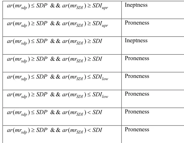
Further the state of given medical record mris assessed as follows:

( _sdp) & & ( _SDI) _upr

ar mr ≤SDP ar mr ≥SDI Ineptness

( _sdp) & & ( _SDI) _upr

ar mr ≥SDP ar mr ≥SDI Proneness

( _sdp) & & ( _SDI)

ar mr ≤SDP ar mr ≥SDI Ineptness

( _sdp) & & ( _SDI)

ar mr ≥SDP ar mr ≥SDI Proneness

( _sdp) & & ( _SDI) _low

ar mr ≤SDP ar mr ≤SDI Proneness

( _sdp) & & ( _SDI) _low

ar mr ≥SDP ar mr ≤SDI Proneness

( _sdp) & & ( _SDI)

ar mr ≤SDP ar mr <SDI Proneness

( _sdp) & & ( _SDI)

[image:10.612.151.456.475.712.2]

ar mr ≥SDP ar mr <SDI Proneness

(11)

Here in the table 2, all possible combinations of SDP and SDI and the impact of those combinations explored. Regardless of the mr_SDI,

if mr_SDPis greater than SDPthen the record confirmed to be Disease Prone. But in contrast, the medical record’s disease ineptness is dependent ofSDP, which is indicating that though the mr_SDIis more than the value of SDI ,

it’s mr_SDPmust be less than the SDP to conclude

that the given medical record mris scaled as disease ineptness. This may leads to slight increase in false positives in prediction but strictly avoids false negatives, which is an accuracy measurement of disease scope.

If ar mr( _sdi)is less than

SDI

and ar mr( _sdp)is

greater than

SDP

, then record is said to be the effected by heart disease.

If disease impacts score of recordmrto be tested is not in the range of disease impacts score of any attack, and hale record score is not in the range of

hale record scope threshold boundaries, then the record said to be normal.

4. EXPERIMENTAL RESULTS AND

PERFORMANCE ANALYSIS

[image:11.612.156.456.444.709.2]

The experiments were carried out on benchmarking dataset that explored in section 3.1. Initially partitioned the processed dataset into normal and diseased records and then the optimal attributes of diseased medical records and normal medical records were traced out, which is by using the process explored (see section 3.2, 3.3, and 3.4). Further the scale to Disease Proneness (SDP) and Scale to Disease Ineptness (SDI) were devised through the process explored (see section 3.5 and 3.6). The exploration of the input data and results were shown in table 3, 4 and 5. The visualization of the optimal scope of attributes for diseased and hale records can be found in fig1 and fig2.

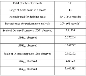
Table 3: Statistics Of The Experiment Results

Total Number of Records 303

Range of fields count in a record 13

Records used for defining scale 80% (242 records)

Records used for performance analysis 20% (61 records)

Scale of Disease Proneness SDP observed 7.11324

low

SDP observed 5.575204

upr

SDP observed 8.651277

Scale of Disease Ineptness SDIobserved 2.982372

low

SDI observed 2.35923

upr

(12)

[image:12.612.84.546.126.685.2] [image:12.612.87.543.130.685.2]

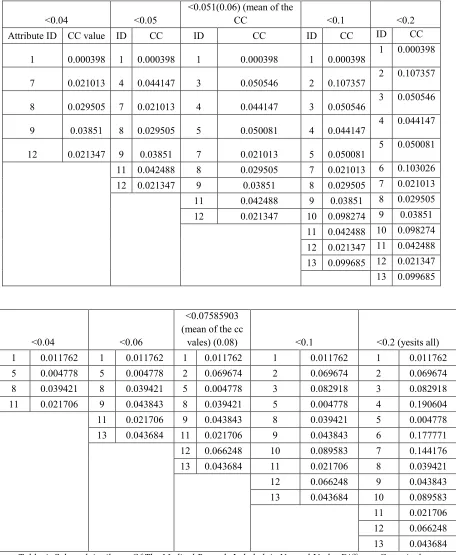
Table 4: Selected Attributes Of The Medical Records Labeled As Diseased Under Different Canonical Correlation Threshold

<0.04 <0.05

<0.051(0.06) (mean of the

CC <0.1 <0.2 Attribute ID CC value ID CC ID CC ID CC ID CC

1 0.000398 1 0.000398 1 0.000398 1 0.000398

1 0.000398

7 0.021013 4 0.044147 3 0.050546 2 0.107357

2 0.107357

8 0.029505 7 0.021013 4 0.044147 3 0.050546

3 0.050546

9 0.03851 8 0.029505 5 0.050081 4 0.044147

4 0.044147

12 0.021347 9 0.03851 7 0.021013 5 0.050081

5 0.050081

11 0.042488 8 0.029505 7 0.021013 6 0.103026 12 0.021347 9 0.03851 8 0.029505 7 0.021013

11 0.042488 9 0.03851 8 0.029505 12 0.021347 10 0.098274 9 0.03851

11 0.042488 10 0.098274 12 0.021347 11 0.042488

13 0.099685 12 0.021347 13 0.099685

<0.04 <0.06

<0.07585903 (mean of the cc

vales) (0.08) <0.1 <0.2 (yesits all) 1 0.011762 1 0.011762 1 0.011762 1 0.011762 1 0.011762 5 0.004778 5 0.004778 2 0.069674 2 0.069674 2 0.069674

8 0.039421 8 0.039421 5 0.004778 3 0.082918 3 0.082918 11 0.021706 9 0.043843 8 0.039421 5 0.004778 4 0.190604 11 0.021706 9 0.043843 8 0.039421 5 0.004778 13 0.043684 11 0.021706 9 0.043843 6 0.177771

12 0.066248 10 0.089583 7 0.144176 13 0.043684 11 0.021706 8 0.039421 12 0.066248 9 0.043843 13 0.043684 10 0.089583 11 0.021706

12 0.066248 13 0.043684 Table 4: Selected Attributes Of The Medical Records Labeled As Normal Under Different Canonical

(13)

[image:13.612.90.523.65.264.2]

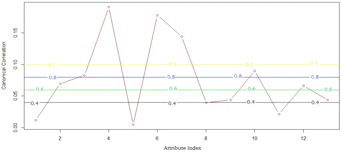
Fig 1: Attributes Of The Medical Records Labeled As Diseased And Their Optimality Under Divergent CC Thresholds

Fig 2: Attributes Of The Medical Records Labeled As Normal And Their Optimality Under Divergent CC Thresholds

4.1 Performance Analysis

The robustness and prediction accuracy of the scales SDPand SDI are assessed through 62 records, which are of the combination of 40 diseased and 22 normal records.

The prediction statistics are as follow:

The count of true positives are (records predicted as truly diseased) 40, the count of true negatives are (records predicted as truly normal) 20, the count of false positives are (records predicted as

falsely diseased) 2 and the count of false negatives are (the records predicted as falsely normal) 0.

[image:13.612.130.479.356.513.2]

(14)

contrast a normal record can be suspected falsely as diseased and may recommend to further diagnosis strategies.

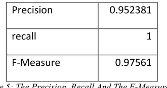
The prediction accuracy of the model devised here in this paper is explored through statistical assessment metrics called precision, recall and f-measure (see table 5). The value obtained for metric recall indicating that the devised model is highly robust and scalable towards assessing disease scope, and the precision also indicating that the prediction accuracy of the model is high and approximately it is 97%.

Precision

0.952381

recall

1

[image:14.612.110.275.270.357.2]

F-Measure

0.97561

Table 5: The Precision, Recall And The F-Measure Of The Predictions

The process time of the application is stable since the increase in number of optimal attributes is not influencing the process complexity (see fig 3)

Fig 3: Process Completion Time Of SDP And SDI Under Divergent Optimal Attributes Selected Through

Various Canonical Correlation Thresholds.

5. CONCLUSION:

This paper introduced a novel heuristic scale to assess the heart disease proneness of the given medical record of an individual patient. In regard to this, two heuristic metrics called Scale to Disease Proneness (SDP) and Scale to Disease Ineptness (SDI) is devised. In contrast to the

existing benchmarking models, the proposed metrics are assessing the disease proneness and ineptness of the medical records SDP and SDI respectively. Further the combinations of these SDP and SDI values of the given medical record are used to assess the state of that medical record. The process opted to devise these metrics is initially finding the optimal attributes of the given diseased and hale medical records, which is done through the canonical correlation analysis. Further the medical records of diseased and hale with optimal attributes are used to assess the metrics SDP and SDI. The experimental results are optimistic and concluding the prediction accuracy and robustness. The future work can be the definition of fuzzy model to estimate the combination of SDP and SDI values.

REFERENCES:

[1] Preventing Chronic Disease: A Vital Investment. World Health Organization Global Report, 2005.

[2] Global Burden of Disease. 2004 update (2008). World Health Organization.

[3] Srinivas, K.,” Analysis of coronary heart disease and prediction of heart attack in coal mining regions using data mining techniques”, IEEE Transaction on Computer Science and Education (ICCSE), p(1344 - 1349), 2010.

[4] Yanwei Xing, “Combination Data Mining Methods with New Medical Data to Predicting Outcome of Coronary Heart Disease”, IEEE Transactions on Convergence Information Technology, pp(868 – 872), 21-23 Nov. 2007

[5] IBM, Data mining techniques, http://www.ibm.com/developerworks/openso urce/library/ba-data-miningtechniques/ index.html?ca=drs- , downloaded on 04 April 2013.

[6] Microsoft Developer Network (MSDN). http://msdn2.microsoft.com/enus/virtuallabs/ aa740409.aspx, 2007.

(15)

[8] Thurai singham, B.: “A Primer for Understanding and Applying Data Mining”, IT Professional, 28-31, 2000.

[9] Han, J., Kamber, M.: “Data Mining Concepts and Techniques”, Morgan Kaufmann Publishers, 2006.

[10]Ho, T. J.: “Data Mining and Data Warehousing”, Prentice Hall, 2005.

[11]C. Aflori, M. Craus, “Grid implementation of the Apriori algorithm Advances in Engineering Software”, Vo lume 38, Issue 5, May 2007, pp. 295-300. A. J.T. Lee, Y.H. Liu, H.Mu Tsai, H.-Hui Lin, H-W. Wu, “Mining frequent patterns in image databases with 9DSPA representation”,Journal of Systems and Software, Volume 82, Issue 4, April 2009, pp.603-618.

[12]Shanta kumar .Patil,Y.S.Kumaraswamy, “Predictive data mining for medical diagnosis of heart disease prediction” IJCSE Vol .17, 2011

[13]M. Anbarasi et. al. “Enhanced Prediction of Heart Disease with Feature Subset Selection using Genetic Algorithm”, International Journal of Engineering Science and Technology Vol. 2(10), 5370-5376 ,2010. [14]Hnin Wint Khaing, “Data Mining based

Fragmentation and Prediction of Medical Data”, IEEE, 2011.

[15]V. Chauraisa and S. Pal, “Data Mining Approach to Detect Heart Diseases”, International Journal of Advanced Computer Science and Information Technology (IJACSIT),Vol. 2, No. 4,2013, pp 56-66. [16]Quinlan J. Induction of decision trees. Mach

Learn 1986; 1:81—106.

[17]Nagavelli, R.; Guru Rao, C.V., "Degree of Disease possibility (DDP): A mining based statistical measuring approach for disease prediction in health care data mining," Recent Advances and Innovations in Engineering (ICRAIE), 2014 , vol., no., pp.1,6, 9-11 May 2014; doi: 10.1109/ICRAIE.2014.6909265

[18]RamanaNagavelli, Dr.C.V.Guru Rao; Degree of Disease Possibility by Feature Correlation (DDP-FC); International Journal of Advanced Computing, ISSN: 2051-0845, Vol.48, Issue.1; RECENT SCIENCE PUBLICATIONS

[19] https://archive.ics.uci.edu/ml/machine-learning-databases/heart-disease/

[20]A. Rencher, Methods of Multivariate Analysis, 2nd ed., Wiley, 2002.

[21]M. Borga, “Canonical correlation: a tutorial”, Linkoping University, Linkoping, Sweden, 2001, 12 pages. Available at http://www.imt.liu.se/∼magnus/cca/tutorial/. [22]A. Hyv¨arinen, J. Karhunen, and E. Oja,

Independent Component Analysis. Wiley, 2001

[23]S. Haykin, Modern Filters. MacMillan, 1989. [24]